Multifractal properties of aperiodic Ising model:
role of the geometric fluctuations

Abstract

The role of the geometric fluctuations on the multifractal properties of the local magnetization of aperiodic ferromagnetic Ising models on hierachical lattices is investigated. The geometric fluctuations are introduced by generalized Fibonacci sequences. The local magnetization is evaluated via an exact recurrent procedure encompassing a real space renormalization group decimation. The symmetries of the local magnetization patterns induced by the aperiodic couplings is found to be strongly (weakly) different, with respect to the ones of the corresponding homogeneous systems, when the geometric fluctuations are relevant (irrelevant) to change the critical properties of the system. At the criticality, the measure defined by the local magnetization is found to exhibit a non-trivial $F(\alpha)$ spectra being shifted to higher values of $\alpha$ when relevant geometric fluctuations are considered. The critical exponents are found to be related with some special points of the $F(\alpha)$ function and agree with previous results obtained by the quite distinct transfer matrix approach.

I Introduction

The introduction of deterministic aperiodicity in the couplings and fields has been intensively used to mimic of the effect of disorder on physical homogeneous systems. This approach, opposed to the more conventional random disorder distribution of coupling constants and fields, has been first used in the analysis of electronic systems, and is now being used to investigate the critical behavior of magnetic systems on Euclidean lattices, as well as on fractal hierarchical lattices.

Hierarchical lattices have been largely used as a framework for analyzing both homogeneous [1] and quenched disordered magnetic systems [2]. It is well known that they offer only crude approximations for the critical properties of the corresponding homogeneous systems on Euclidean spaces with the same fractal dimension, but they provide an useful tool to investigate, via exactly solvable models, the effect of both random and deterministic disorder. For instance, the short range Ising spin glass model defined on the diamond hierarchical lattice has been analyzed by means of a methodology that encompasses an exact real space renormalization group decimation and an exact recursive procedure to calculate the local magnetization of all lattice sites for a particular realization of the disorder (sample)[3]. A detailed numerical investigation reveals that the multifractal properties of the local Edwards-Anderson (EA) order parameter remains non-trivial far below the critical temperature. This contrasts with previous investigations of the homogeneous pure ferromagnetic Ising model on the same lattice, for which the multifractal spectra of the normalized local magnetization survives only at the critical temperature [4, 5]. Concerning the critical behavior of the Ising spin glass model, it was possible to obtain strong evidences of universal critical exponents and a unique value for the temperature of the critical point when several probability distributions for the quenched coupling constants are considered [6, 7]. It is worth to mention that the values of the critical temperature and of the critical exponents associated to the order parameter and correlation length for Ising spin glass model on diamond hierarchical lattice with graph fractal dimension $d_{F}=3$ are surprisingly close to those obtained by numerical simulations for the model defined on cubic lattices [8].

In a recent publication, Luck [9] proposed a heuristic criterion to account whether the geometric fluctuations in coupling constants and fields are relevant or irrelevant to alter (or not) the universality class of the aperiodic systems with respect to the corresponding homogeneous one. Luck’s criterion plays the similar role of that due to Harris [10], that holds when quenched disorder is introduced in ferromagnetic systems. In the latter, the critical behavior is changed provided the critical exponent associated with the divergence of the specific heat of the corresponding homogeneous system is positive. More recently, an exact derivation of an analog of the Luck’s criterion was presented for both the Ising [11] and the Potts [12, 13] models, defined on the family of diamond hierarchical lattice filled with aperiodic interactions dictated by a generalized Fibonacci sequence. Using the transfer matrix (TM) approach, Andrade [14] obtained exact numerical results for the thermodynamic and critical properties of the aperiodic ferromagnetic Ising model defined on the family of diamond hierarchical lattices (hereafter DHL), corroborating the change of universality class of the model when relevant geometric fluctuations are considered accordingly to the Luck’s like criterion properly adapted to cope with hierarchical lattices. We notice that the exact scale invariance symmetry is the crucial property of the DHL’s underlying the methods which link the thermodynamic functions of lattices with successive generations, as occurs for the above mentioned real renormalization group scheme as well as for transfer matrices approach [14].

In this work we are mainly interested to investigate the role of geometrical fluctuations on the multifractal properties of the local magnetization of ferromagnetic Ising model on the DHL’s. We focus our study on two distinct models, both defined on DHL’s with the same graph fractal dimension but with distinct topologies leading to relevant and irrelevant fluctuations. To deal with the multifractal properties of the local magnetization we apply the methodology developed to study the multifractal spectra of the order parameter of the homogeneous ferromagnetic Ising model [4, 5, 15] and the spin-glass Ising model [7] on the DHL’s. As we will show, the caracter of the fluctuations influences the nature of the changes observed in the singularity spectrum of the local magnetization.

In section II, we describe the model Hamiltonian, present the sequences governing the aperiodic interactions and discuss the relevance of the geometric fluctuations for both lattices, accordingly with the appropriated criterion presented in [11]. We also review the main features of the flow diagram and the phase diagram of the aperiodic systems. Section III is devoted to review the method to obtain the local magnetization and to discuss the multifractal spectra for special realizations of the geometric fluctuations. Finally we discuss and summarize our main conclusions in section IV.

II The model Hamiltonian and the aperiodic interactions

A general hierarchical lattice is constructed according to a recursive rule where some bonds of basic unit are successively replaced by the basic unit itself. The general basic unit of the diamond hierarchical lattices $(b,p)$-DHL, is formed by two roots sites connected by a set of $p$ parallel branches, each one containing a series of $b$ connected bonds. A given generation is obtained by replacing all bonds of the previous generation by the basic unit, as sketched in Figure 1. For this family of hierarchical lattices, the graph fractal dimension is given by $d_{F}=1+\log p/\log b$, while its size, number of sites and the number of bonds are respectively given by $L=b^{N}$, $N_{S}=(b-1)p[(bp)^{N}-1]/(bp-1)$ and $N_{B}=(bp)^{N}$, $N$ being the number of generations.

The reduced Hamiltonian for the system is

$$-H/k_{B}T=\sum\limits_{\left\langle i,j\right\rangle}K_{ij}\sigma_{i}\sigma_{j}\ ,$$ (1)

where $\sigma_{i}=\pm 1$ are the Ising variables and the sum runs over all pairs of nearest neighbors spins $\left\langle i,j\right\rangle$ , $K_{ij}=J_{ij}/k_{B}T$ are the corresponding coupling constants, $k_{B}$ is the Boltzmann constant and $T$ is the absolute temperature.

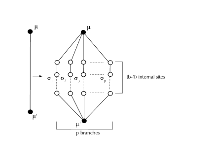
FIG. 1.: Basic unit of the general diamond hierarchical lattice $(b,p)$-DHL with $p$ parallel branches each one with $b-1$ connected internal sites.

In this paper, we consider geometric fluctuations introduced by the generalized Fibonacci inflation rule expressed by

$$(A,B)\rightarrow(AB^{b-1},A^{b})\ .$$ (2)

When applied to define the coupling constants of the hierarchical lattice $(J_{ij}=J_{A};J_{B})$, the above rule corresponds to the following procedure: $(a)$ a bond with coupling constant $J_{A},(J_{A}>0)$ should be replaced by a basic unit with $p$ parallel branches each one containing the first bond with coupling constant $J_{A}$ and the next $(b-1)$ ones with coupling constants $J_{B}$; $(b)$ a bond $J_{B},(J_{B}>0)$ should be replaced by a basic unit with all bonds with coupling constants $J_{A}$. This correspondence is displayed in Figures 2a and 2b, for the cases of the lattices with $p=b=2$ and $3$, respectively. After N steps, the length of the aperiodic sequences on which we base the present definition of the geometric fluctuations is given by $b^{N}$, which corresponds to the number of bonds within each one of the shortest paths connecting the two root sites and measures the size of the lattice. We also notice that there are $p^{N}$ of such shortest paths, all of them with no common bonds and showing the same aperiodic sequence. Therefore the systems can be regarded as formed by identical layers with the bonds $J_{A}$ and $J_{B}$ arranged accordingly to the sequence (2). The number of distinct letters or coupling constants within two subsequent generations of the sequence are related by the substitution matrix $M$ given by

$$M=\left[\matrix{1&b\cr b-1&0\cr}\right],$$ (3)

whose eigenvalues are $\lambda_{1}=b$ and $\lambda_{2}=(1-b)$. The wandering exponent which measures, the fluctuation in the distribution of elements within the sequence, is defined as

$$\omega=\frac{\log\left|\lambda_{2}\right|}{\log\lambda_{1}}.\$$ (4)

The sequences defined by (2) are said to be non-Pisot if $\omega>0$ ($b>2$), which means that the fluctuations are unbounded, whereas the case $\omega=0$ ($b=2$) corresponds to marginal case. On the other hand, for the Ising model on DHL with aperiodic interactions arranged by sequences such that $\lambda_{1}=b$, the geometric fluctuations are said to be relevant provided

$$\omega>\omega_{c}=1-1/\nu,$$ (5)

$\nu$ being the critical exponent associated with the correlation length of the homogeneous system [11].

In the present work we consider two models: model 1 is defined on a $(2,2)$-DHL while model 2 is defined on a $(3,3)$-DHL.

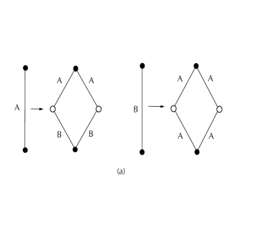
FIG. 2.: Basic units of the (a) $(2,2)$-DHL and (b) $(3,3)$-DHL indicating the distribution of couplings $J_{A}$ and $J_{B}$ accordingly with the generalized Fibonacci sequences.

The corresponding lattices have been choosen to have the same fractal dimension ($d_{F}=2$), but the geometric fluctuations are respectively irrelevant and relevant respectively accordingly to eq.(5), as has been demonstrated by Pinho et al [11]. In the rest of this section we review the basic properties of the renormalization flow of the model Hamiltonian in these lattices.

Consider a general $(b,p)$-DHL with the coupling constants defined by the inflation rule given by (2). Within the real space renormalization group scheme, the decimation procedure is carried on by partial tracing on the spins introduced in the last generation. This leads to exact scaling relations for the coupling constants $J_{A}$ and $J_{B}$, given respectively the following renormalization equations:

$$t_{A}^{\prime} = \tanh[p\tanh^{-1}(t_{A}t_{B}^{b-1})]$$ (6)

$$t_{B}^{\prime} = \tanh[p\tanh^{-1}(t_{A}^{b})]$$ (7)

where $t_{x}=\tanh K_{x},$ $\ x=A$ or $B$.

The renormalization flow diagram in the $(t_{A},t_{B})$ space has been carefully studied in [11, 13]. The equations (6) have three fixed point solutions, all of them located along the manifold $t_{A}=t_{B}$: $t_{\infty}^{*}=0$, $t_{0}^{*}=1$, and $t_{c}^{*}$. Therefore, they are also the solutions of the corresponding homogeneous system. The first two solutions refer to stable fixed points corresponding to the infinite (paramagnetic) and zero (ferromagnetic) temperature phases respectively while the third one is associated with the critical point governing the transition of the corresponding homogeneous system. For the particular models considered here, these critical point solutions are exact and given by,

$$t_{c1}^{*} = \frac{1}{3}(a_{c}-2/a_{c}-1)=0.543689...\text{ for }p=b=2$$ (8)

$$t_{c2}^{*} = \frac{1}{2}(\sqrt{5}-1)=0.618033...\text{ for }p=b=3$$ (9)

where $a_{c}=(3\sqrt{33}+17)^{\frac{1}{3}}$. As shown in [11], the renormalization flow space has two regions corresponding to the basins of attraction of the stable fixed points. The frontier of these regions, containing the critical point of the homogenous system, determines the phase diagram. However, as pointed out in [11, 12, 13], linearization about the non-trivial fixed point indicates that it is a saddle-point for lattices with $b=2,(\omega=0<\omega_{c})$, while it becomes fully unstable for lattices with $b>2,(\omega>\omega_{c})$. Therefore, for model 1 the critical behavior should be governed by the fixed-point of the homogeneous system and the geometric fluctuations are irrelevant with respect to change the universality class of the model. On the other hand, for model 2, the non-trivial fixed point is fully inaccessible indicating that the geometric fluctuations are indeed relevant to change the critical behavior. To grasp the critical behavior of the relevant aperiodic model one should explore further the flow diagram given by eqs.(6). This was already done by Haddad et al [13] investigating the Potts model on the $(3,2)$-DHL. Actually, whenever the fixed-point becomes fully unstable, they found the appearance of a two-cycle attractor associated with the novel critical behavior. For the present model 2, this two-cycle attractor is given by coordination points ($t_{A1}^{*}=0.95116...,t_{B1}^{*}=0.46135...$) and ($t_{A2}^{*}=0.54822...,t_{B2}^{*}=0.99915...$) [16].

In Figure 3, we show the $(t_{A},t_{B})$ flow diagram for the $p=b=3$ case. Note that thetwo-cycle attractor is a saddle-point being unstable towards the trivial stable fixed-points and stable in the perpendicular direction.

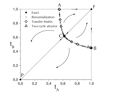
FIG. 3.: The flow diagram in the $t_{A}\times t_{B}$ space for the real space renormalized couplings for model 2. The arrows indicates the flow of the second iterates. F and P denote the stable fixed-points corresponding to the ferromagnetic and paramagnetic phases. C labels the fully unstable fixed-point. $\triangle$ locates the two-cycle attractor and $\diamond$ the critical points obtained by the transfer matrix method. $\times$ labels the critical points obtained by inverting the renormalization equations. A and B give the frontiers of the basin of attraction within the manifolds $t_{B}=1$ and $t_{A}=1$ respectively

The frontier between the basin of attraction of the stable fixed-points contains both the two-cycle attractor and the fully unstable fixed-point. This frontier intersects the lines $\ t_{B}=1$ and $t_{A}=1$ in two points, respectively $A$ and $B$, and it manifold is associated with the critical temperatures of the model for different choices of the ratio $R=J_{B}/J_{A}$.

The flow diagram can be numerically obtained by inverting eqs.(6) taking into account that the inverse equations share the same trivial, non-trivial fixed points and two-cycle attractor as eqs.(6), but with inverted unstable to stable manifolds and vice-versa. So, the iterates of these inverted equations starting close to the critical fixed point are now pushed towards line $ACB$, so that a relation $t_{B}=g(t_{A})$ can be numerically obtained ending to the phase diagram.

In Figures 4a and 4b, we draw such relation in the $(T/J_{A},R)$ phase diagrams of both models, indicating the critical temperature obtained for some special values of the ratio $R$ by using the TM formalism [14], as well as the corresponding exact values for the homogeneous models ($R=1$). The critical exponent $\nu$ associated with the correlation length of the corresponding homogeneous systems can be exactly calculated as

$$\nu=\frac{lnb}{lnr_{c}}$$ (10)

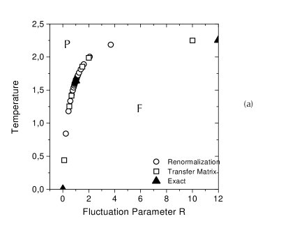
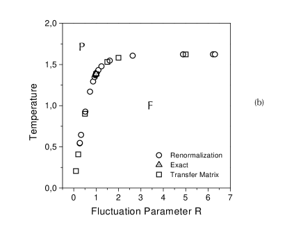
FIG. 4.: Phase diagram $K_{B}T/J_{A}\times J_{B}/J_{A}$ for (a) model 1, (b) model 2. $\bigcirc$ ($\bullet$) indicate numerical (exact) values obtained with the present methodology , while $\triangle$ indicate values obtained by transfer matrix method. $\triangle$ label the exact values for the homogeneous systems

where

$$r_{c}=\left|{\frac{dt^{\prime}(t)}{dt}}\right|_{t=t_{c}^{*}}\\ ={\frac{4bpt_{c}^{*b}(1+t_{c}^{*b})^{p-1}(1-t_{c}^{*b})^{p-1}}{((1+t_{c}^{*b})^{p}+(1-t_{c}^{*b})^{p})^{2}}},$$ (11)

and $t^{\prime}(t)$ is given by eqs.(6) when $t_{A}=t_{B}=t$.

TABLE I.: Exact values for $\nu$, $\omega$ and $\omega_{c}$ for models 1 and 2.

	model 1	model 2
$\nu$	1.338265788…	1.779416044…
$\omega$	0	0.630929753…
$\omega_{c}$	0.252764279…	0.438017880…

In Table I, we show the values of $\nu$, $\omega$ and $\omega_{c}$ for models 1 and 2. It corroborates that for model 2 we have $\omega>\omega_{c}$ indicating that the geometric fluctuation should be relevant for this model.

III The Local Magnetization

The method of evaluation the local magnetization is based on the assumption that the model Hamiltonian for a lattice with $N$ generations is equivalent to a reduced effective Hamiltonian of a single basic unit introduced in the $N^{th}$ step plus effective fields acting on the spins of its external sites and an effective interaction coupling these spins. This assumption, which has been proved to be formally correct for the homogeneous system, also holds for the present model, since no special condition is imposed to the coupling constants of the Hamiltonian. These unknown local effective interaction and fields represent the influence of the remaining lattice spin couplings transmitted by the external spins of that basic unit. The local magnetization of both internal and external sites of the basic unit of the effective system are calculated as a function of coupling constants $(J_{A}$ and $J_{B})$ and the unknown effective coupling and fields. Eliminating the unknown variables we end up to recursive relations for the local magnetization of the internal sites in terms of the corresponding values of the root sites. Now, considering a $N$ generation lattice and successively decimating the spins up to the first generation (basic unit) one can recursively calculate the local magnetization by choosing appropriated values for the magnetization of root sites, accordingly with the configuration of the phase of the corresponding fixed point. In [4] the details of the calculations of the recursive equations for the uniform ferromagnetic case is presented, while in [3] these equations were generalized for basic unit with arbitrary interactions in order to investigate the short range Ising spin glass model. The recursive equations for the latter can be straightforwardly applied to deterministic aperiodic Ising models expressing the site magnetization of internal sites $\left\langle\sigma\right\rangle$ in terms of the corresponding values for the external sites. The recursive expression for model 1 is given by :

$$\left\langle\sigma\right\rangle=A_{1}\left\langle\mu\right\rangle+B_{1}\left\langle\mu^{\prime}\right\rangle$$ (12)

where

$$A_{1} = \frac{t_{A}(1-t_{A}t_{B})}{(1-t_{A}^{2}t_{B}^{2})},$$ (13)

$$B_{1} = \frac{t_{B}(1-t_{A}t_{B})}{(1-t_{A}^{2}t_{B}^{2})},$$ (14)

for the $(AB)$ non-homogeneous basic unit while

$$A_{1}=B_{1}=\frac{t_{A}}{(1+t_{A}^{2})}$$ (15)

for the $(A,A)$-homogeneous basic unit, as specified in Figure 2a.

On the other hand, for model 2 we have two sets of recursive equations obtained for each one of the basic units shown in Figure 2b. Each set has two equations corresponding to the internal sites of each basic unit. For the non-homogeneous basic unit (ABB) these equations are given by

$$\left\langle\sigma_{i}\right\rangle=A_{i}\left\langle\mu\right\rangle+B_{i}\left\langle\mu^{\prime}\right\rangle\hskip 85.35826pt(i=1,2),$$ (16)

where

$$A_{1} = \frac{t_{A}(1-t_{B}^{4})}{(1-t_{A}^{2}t_{B}^{4})},$$ (17)

$$B_{1} = \frac{t_{B}^{2}(1-t_{A}^{2})}{(1-t_{A}^{2}t_{B}^{4})},$$ (18)

$$A_{2} = \frac{t_{A}t_{B}(1-t_{B}^{4})}{(1-t_{A}^{2}t_{B}^{4})},$$ (19)

$$B_{2} = \frac{t_{B}^{2}(1-t_{A}^{2}t_{B}^{2})}{(1-t_{A}^{2}t_{B}^{4})},$$ (20)

while for the homogeneous basic unit (AAA) they are expressed by

$$\left\langle\sigma_{i}\right\rangle=C_{i}\left\langle\mu\right\rangle+D_{i}\left\langle\mu^{\prime}\right\rangle\hskip 85.35826pt(i=1,2),$$ (21)

where

$$C_{1}=D_{2}= \frac{t_{A}(1-t_{A}^{4})}{(1-t_{A}^{6})},$$ (22)

$$D_{1}=C_{2}= \frac{t_{A}^{2}(1-t_{A}^{2})}{(1-t_{A}^{6})}.$$ (23)

To evaluate the correct value of the local magnetization $m_{i}=\left\langle\sigma_{i}\right\rangle$ of each site, it is necessary to keep track of its local interaction configuration, i.e., to know with which choice of $J_{A}$ and $J_{B}$ a given inner spin interacts with its root sites. In order to breakdown the global up-down symmetry and obtain non-zero values for the spontaneous magnetization, it is enough to apply a field on a given site of the lattice and let this local field equal zero at the end of calculation. However, within the present methodology this breakdown is easily done by assuming boundary conditions to root sites accordingly with the corresponding configuration of the stable fixed-point phase. This latter procedure is followed in the present work.

Now we focus our attention to model 2 looking over the effects of the relevant geometric fluctuations with regard to the homogeneous pure model on the same lattice. First, we consider the local magnetization of the sites along one of the shortest path connecting the root sites. These values are assigned to points within the interval $[0,1]$, since the DHL is a fractal graph where the bonds mean ”chemical distances” without any geometric sense. The resulting plot gives a representative picture of the local magnetization distribution, hereafter called magnetization profile, since all shortest path are equivalent as far the DHL graph symmetry is concerned. Figure 5a shows the magnetization profile for the homogeneous model 2 at the critical temperature of the corresponding saddle-point fixed-point, and Figures 5b and 5c show the profiles for the aperiodic model 2 at the critical temperatures of each one point of the two-cycle attractor for (which correspond to fluctuation parameter values $R_{c1}=J_{B}/J_{A}=0.2706...$ and $R_{c2}=J_{B}/J_{A}=6.3104...$. For the first profile, in any of the renormalization steps, the coefficients (17,22) have their values fixed by the corresponding value at the critical point. For the other two profiles these coefficients alternate between the corresponding values at the two-cycle attractor. For values of $J_{A}$ and $J_{B}$ other than those corresponding to the critical sets, the present methodology produces the local magnetization as function of the temperature, but the above mentioned coefficients evolve under the renormalization process. In any case, the magnetization of the global root sites are held fixed with initial values equal to one, which corresponds to the ferromagnetic configuration.

All profiles shown display many singularities and are, in some sense, self similar. However those of the aperiodic system clearly do not show the same symmetries as the one from the homogeneous model ($R=1$). As pointed out in [4, 5], for the homogeneous model the pattern symmetries are solely related with the topologic symmetry of the lattice, imposed by the distribution of coordination numbers along the profile. However, for the aperiodic systems, the self similar symmetry of the lattice topology is superimposed by symmetries of the aperiodic sequence defining the distribution of interactions, so that the resulting pattern expresses the influence of both symmetries. We emphasize that this feature does not depend on the relevant-irrelevant character of the fluctuations, and is observed also for the aperiodic situation of model 1. It is worth to comment that for the spin-glass model the symmetry induced by the lattice topology is completely washed out by the random quenched disorder of the coupling constants [3].

The profiles in Figures 5b and 5c are, at first sight, rather different, but a close analysis uncover the fact that they share the same structure. We note also the presence of two different scales corresponding to the regions where the letters $A$ and $B$ are more abundant. As the values of $J_{A}$ and $J_{B}$ are rather distinct for the two points of the cycle, they enhance or depress the values of the local magnetization in these regions, leading to the two different shapes.

It is important to observe that both profiles were obtained after eight generations, so that, in the flow diagram, the trajectories start and end at the same point of the cycle.

If we consider an odd number of generations the form of the profiles would be reversed, indicating that the profile does not converge to a single form, but rather oscillates between two distinct patterns which reflect the properties of each of the points in the cycle. The same behavior is observed for every profile, evaluated with any choice of values for $J_{A}$ and $J_{B}$, at the corresponding value of $T_{c}$.

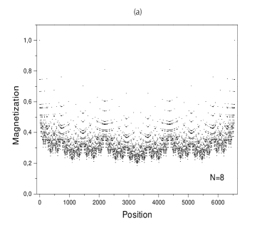
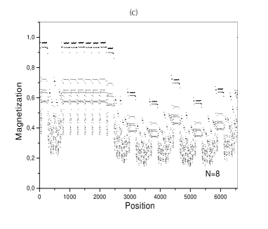
FIG. 5.: Magnetization profiles patterns of the model 2 for lattices with $N=10$ hierarchies at the criticality. (a) $R=1$ homogeneous system, (b) $R_{c1}=0.2706...$ and (c) $R_{c2}=6.3104...$ aperiodic systems at the fixed-points of the two-cycle attractor, respectively.

As this alternating form of the profile pattern results from the different properties of the two points of the cycle, it is not observed in the case of irrelevant fluctuations. Indeed, for any value of $J_{A}$ and $J_{B}$, the trajectory at the corresponding $T_{c}$ is controlled by the properties of the critical point of the homogeneous system: the profile converges to a definite form, with a lower symmetry than in the case of the homogeneous system.

As previously observed for the homogeneous cases [4], the high degree of singularities suggests the multifractal analysis as a valuable tool to investigate the structure of the magnetization profiles for the models with $R\neq 1$. The $F(\alpha)$ functions of the measure defined by the normalized local magnetization $\mu_{i}(L)=m_{i}(L)/\sum_{j}m_{j}(L)$ were calculated by the method due to Chhabra and Jensen [17] which is based on a one parameter family of normalized measures,

$$\xi_{i}(q,L)={\frac{\mu_{i}(L)^{q}}{\sum_{j}[\mu_{j}(L)]^{q}}.}$$ (24)

In Figures 6a and 6b we show the plots for both models comparing the $F(\alpha)$ spectra of the aperiodic and the homogeneous system at criticality. Both curves have the same maximum value ($F(\alpha)_{max}$=1) since the measure has been arbitrarily assigned to the interval $[0,1]$, that is, to the same fractal set (support) of dimension $d=1$. Therefore, one must focus our attention to the values of the H$\ddot{o}$lder exponent $\alpha$. The minimum and the maximum values of $\alpha$ reflect, respectively, how the measures of the most concentrated and the most rarefied intervals scale with the box width. For the homogeneous systems the domain of the $F(\alpha)$ spectra can be analytically calculated [15]. Moreover as was demonstrated in [5, 15] there is a straightforward relation between the H$\ddot{o}$lder exponent and the critical exponents given by

$$\alpha=d+\frac{1}{\nu}(\beta_{\alpha}-\beta)$$ (25)

where $d$ is the fractal dimension of the support and $\beta_{\alpha}$ is the critical exponent associated with the average magnetization of the subset of sites whose the measure vanishes with exponent $\alpha$, as $L\rightarrow\infty$. Since the most concentrated measures of both models have finite values at the thermodynamic limit induced by the boundary conditions we have $\beta_{\alpha_{min}}=0$ and $\alpha_{min}=d-\beta/\nu$. Therefore $\alpha_{min}$ is solely related with the exponents describing the critical behavior of the whole system and should follows the rules for the universality class of the systems. Moreover, for the subset of sites where the measure behaves with the H$\ddot{o}$lder exponent $\overline{\alpha}=d$, the local magnetization behaves with the same critical exponent of the average magnetization of whole lattice, that is, $\beta_{\overline{\alpha}}=\beta$. This particular subset should also follow the rules of the universality class, and therefore the point $(d,F(d))$ on the $F(\alpha)$ function should remains fixed when irrelevant geometric fluctuations are considered.

From Figure 6b, it becomes clear that the aperiodic systems with relevant geometric fluctuations belong to a distinct class of universality regarding the homogeneous system, as the $F(\alpha)$-function of the former is shifted to higher values of $\alpha$. Moreover, we notice two distinct $F(\alpha)$ spectra, corresponding to distinct profiles with $R=1$ and $R\neq 1$.

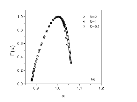
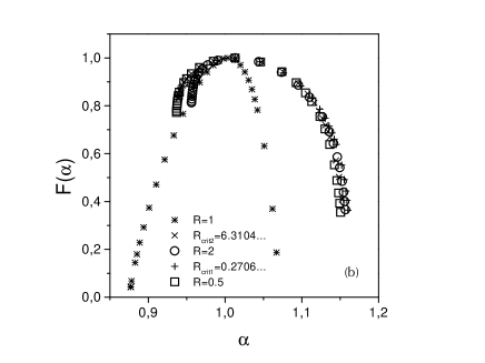
FIG. 6.: F($\alpha$) spectra of the normalized magnetization hierarchies at the criticality. (a) model 1 for lattices with $N=20$ and $q\in[-60,60]$. $\ast$ labels the spectrum of the corresponding homogeneous systems, $\bigcirc$ the $R=2$ aperiodic system and $\Box$ the $R=0.5$ aperiodic system . (b) model 2 for lattices with $N=15$ and $q\in[-40,50]$, $\ast$ labels the spectrum of the corresponding homogeneous systems, $\bigcirc$ and $\Box$ the spectrum of the $R=2$ and $R=0.5$ aperiodic system respectively . $+$ and $\times$ label the spectrum of the $R_{c1}=0.2706...$ and $R_{c2}=6.3104...$ fixed-points of the two-cycle attractor, respectively.

On the other hand, as displayed in Figure 6a the $F(\alpha)$ functions of model 1 with $R=0.5$ and $2$ suffer minor changes due to finite size effects when compared with the one for $R=1$. To handle with such differences we refine our calculations by doing a finite size scaling estimation of the values of $\alpha$ and $F(\alpha)$ for higher $|q|$, and by proceeding a finite size scaling estimation of the exponent $\phi$ governing the average magnetization at the critical point $m\sim L^{-\phi}$,which by it turn is related with the critical exponents by $\phi=\beta/\nu$.

In Tables II and III, we present these estimations for both models respectively, comparing with exact values whenever is possible. We notice the slight difference when the $\alpha_{min}$ of the aperiodic system of model 1 is compared with the exact value for the homogeneous system, indicating conservation of universality (see Table II). However, for model 2, qualitative differences are observed when the $\alpha_{min}$ values of the aperiodic and the homogeneous models are compared. In this latter case the values of $\alpha_{min}$ oscillates as we go from $N$ even to $N$ odd lattices. As pointed out in our former discussion, these oscillations are a manifestation of the fact that the profile oscillates between two different patterns dictated by the properties of each of the points of the cycle. In Figure 7 we present the scaling for the $\alpha_{min}$ of the F($\alpha$) function of model 2 for some values of the fluctuation parameter $R$. For $R_{c1}$ and $R_{c2}$ these oscillations are clearly seen as we go from $N$ even to $N$ odd lattices. For finite lattices and finite values of $q$, the oscilations on the scaling plot introduce significant errors bars for thevalues of the corresponding exponents. However, as $N$ goes to infinity, we expect that $\alpha_{min}$ converges to a unique universal limit for any value of the fluctuation parameter other than $R=1$.

In Table III, we also compare the values of $\alpha_{min}$ obtained within the present approach with the ones deduced from the results for $\beta/\nu$, calculated using the transfer matrix approach developed by one of us [14]. It is worth to mention that this latter approach allows to work with higher values of $N$, ending up with more accurate values for the exponents.

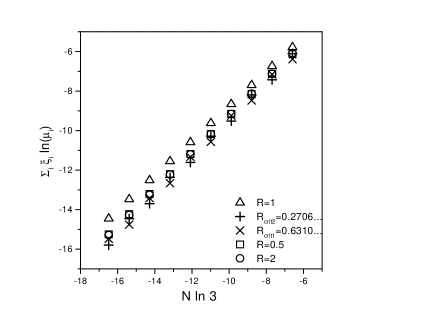
FIG. 7.: Scaling of the $\alpha_{min}$ of the $F(\alpha)$-function of model 2 for values of $R=1$, $R=0.5$, $R=2$, $R_{c1}=0.2706...$ and $R_{c2}=6.3104...$. The corresponding exponents are given on table III.

IV Summary and conclusions

We investigate the role of the geometric fluctuations on the local magnetization and critical properties of the ferromagnetic Ising model when the coupling constants are defined by deterministic aperiodic sequences. Two distinct models were considered as a matter of comparation. Model 1 (model 2) was build with irrelevant (relevant) Fibonacci like geometric fluctuations with respect to changes in the critical properties. The models are defined on different diamond hierarchical lattices but with then same fractal dimension $d_{F}=2$. The phase diagram of both models were obtained and carefully analyzed. The local magnetization of both models was calculated by an exact recurrence procedure as function of the temperature but we concentrate our analysis close to the critical point. When the relevant (irrelevant) geometric fluctuation is concerned the pattern of the local magnetization profile exhibit a strong (weak) change of it symmetry as compared with the one of the corresponding homogeneous system. For the model 1, the self-similar pattern induced by the lattice topology is predominant, as it occurs for the homogeneous system.

However, for model 2, the pattern symmetry of the homogeneous system is strongly affected by the one dictated by aperiodic distribution of coupling constants and the local magnetization profile resulting with a quite different distribution of singularities. This break of symmetry is straightforwardly related with the change in critical properties, as revealed by the multifractal analysis of the magnetization profiles at the criticality. The $F(\alpha)$-functions of the model 1 is quite close to the one of the corresponding homogeneous systems for all values of domain of the spectrum, reflecting the same critical behavior of the latter. However, the domain of the $F(\alpha)$-functions of the model 2 is shifted to higher values of $\alpha$, with respect to the one of the corresponding homogeneous systems, leading to change the universality class of the model regarding the relative values of the ferromagnetic coupling constants. The critical exponent associated with the magnetization of model 2 were calculated by means of the $F(\alpha)$-function as well as by scaling the average magnetization. The results are in good agreement with the ones obtained through the thermodynamic functions calculated using a quite different approach previously developed by one of us. Therefore, we have demonstrated, by means of exact numeric calculations of the local magnetization of useful models, that as far as relevant deterministic geometric fluctuations is concerned the resulting disorder in the distribution of aperiodic ferromagnetic interactions leads to a strong break of symmetry in the patterns of the local magnetization following the change of universality class.

TABLE II.: Domain of the F($\alpha$) spectra for the aperiodic and homogeneous systems for model 1. The numerical values obtained by the scaling of $\alpha_{min}$ and $\alpha_{max}$ of the aperiodic systems were calculated for lattices with N=10 to 22 and for $q=\pm 50$. The finite size scaling of the average magnetization was performed for lattices with $L=2^{N}$, $N=10$ to $22$.

method		R=1	R=2	R=0.5
analytic a	$\alpha_{mim}$	0.8791464205	–	–
scaling b	$\alpha_{mim}$	0.87895(6E-5)	0.8793(9E-4)	0.876(E-3)
scaling b	$1-\beta/\nu$	0.87900(3E-5)	0.8794(9E-4)	0.879(E-3)
transfer matrix c	$1-\beta/\nu$	0.87915(E-5)	–	–
analytic a	$\alpha_{max}$	1.04604781…	–	–
scaling b	$\alpha_{max}$	1.03920(7E-5)	1.0467(6E-4)	1.0474(5E-4)

TABLE III.: Domain of the F($\alpha$) spectra for the aperiodic and homogeneous systems for model 2. The numerical values obtained by the scaling of $\alpha_{min}$ and $\alpha_{max}$ of the aperiodic systems were calculated for lattices with N=6 to 15 and for $q=\pm 40$. The finite size scaling of the average magnetization was performed for lattices with $L=3^{N}$,$N=6$ to $15$.

method		R=1	R=6.3104…	R=0.2706…	R=2.0	R=0.5
analytic d	$\alpha_{mim}$	0.8760357586…	–	–	–	–
scaling e	$\alpha_{mim}$	0.8768(5E-4)	0.95(E-2)	0.94(E-2)	0.9314(7E-4)	0.9219(8E-4)
scaling b	$1-\beta/\nu$	0.8768(5E-4)	0.95(E-2)	0.94(E-2)	0.9301(6E-4)	0.9178(6E-4)
transfer matrix f	$1-\beta/\nu$	0.8760(E-4)	0.95481(E-5)	0.955(E-3)	–	–
analytic a	$\alpha_{max}$	1.068947633..	–	–	–	–
scaling b	$\alpha_{max}$	1.0643(6E-4)	1.1660(5E-4)	1.162(5E-3)	1.166(5E-3)	1.160(5E-3)

REFERENCES

- [1] For a recent review on hierarchical lattices, see C. Tsallis and A. C. N. Magalhães, Phys. Rep. 268, 305 (1996).
- [2] B. W. Southern and A. P. Young, J. Phys. C Solid State 10, 2179 (1977).
- [3] E. Nogueira Jr., S. Coutinho, F. D. Nobre, E. M. F. Curado and J. R. L. de Almeida, Phys. Rev. E 55, 3934 (1997).
- [4] W. A. M. Morgado, S. Coutinho and E. M. F. Curado, J. Sta. Phys. 61, 913 (1990).
- [5] W. A. M. Morgado, E. M. F. Curado and S. Coutinho, Rev. Bras. Fis. 21, 247 (1991).
- [6] E. Nogueira Jr., S. Coutinho, F. D. Nobre and E. M. F. Curado, Physica A 257, 365 (1998).
- [7] E. Nogueira Jr. , S. Coutinho, F. D. Nobre, E. M. F. Curado, Physica A, 271, 125, (1999).
- [8] S. Prakash and I. A. Campbell, Physica A 235, 507 (1997).
- [9] J. M. Luck, Europhys. Lett. 24, 359 (1993); J. Stat. Phys. 72 417 (1993).
- [10] A. B. Harris, J. Phys. C Solid State 7, 1671 (1974).
- [11] S. T. R. Pinho, T. A. S. Haddad and S. R. Salinas, Physica A 257, 515 (1998); Bras. J. Phys. 27, 567 (1997).
- [12] A. C. N. Magalhães, S. R. Salinas and C. Tsallis, Physica A 31, L567 (1998).
- [13] T. A. S. Haddad, S. T. R. Pinho and S. R. Salinas, Phys. Rev. E 61, 3330 (2000).
- [14] R. F. S. Andrade, Phys. Rev. E 59, 150 (1999)
- [15] S. Coutinho, O. Donato Neto, J. R. L. de Almeida, E. M. F. Curado and W. A. M. Morgado, Physica A 185, 271 (1992).
- [16] T. A. S. Haddad, MSc. Thesis, Universidade de São Paulo (1999).
- [17] A. Chhabra and R. V. Jensen, Phys. Rev. Lett. 62, 1327 (1989).