The Theory of Atom Lasers

Abstract

We review the current theory of atom lasers. A tutorial treatment of second quantisation and the Gross-Pitaevskii equation is presented, and basic concepts of coherence are outlined. The generic types of atom laser models are surveyed and illustrated by specific examples. We conclude with detailed treatments of the mechanisms of gain and output coupling.

1 Introduction

An atom laser is a device which produces a bright, directed, and coherent beam of atoms. An ideal atom laser beam is a single frequency de Broglie matter wave, approximating a noiseless sinusoidal wave; in particular it will have a well defined frequency, phase, and amplitude. Quantum mechanically, such a wave is a mode of the quantised field, and the properties of brightness and well defined phase require the mode to be highly occupied. This is equivalent to requiring Bose degeneracy, and rules out the possibility of a fermionic atom laser[1].

Atom lasers are a recent concept, and to our knowledge the earliest scientific description appeared in 1993 [2]. The first comprehensive papers on matter wave amplification[3] and atom lasers[4, 5, 6] appeared in 1995, and the first experimental demonstration of an atom laser in 1997 [7]. The essential components of an atom laser have been identified by analogy with optical lasers and are illustrated in Fig. 1.

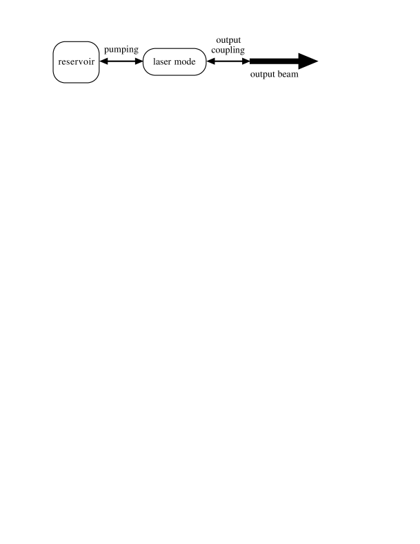
Figure 1: Schematic diagram of a generic atom laser.

They are; a reservoir of atoms from which the laser is pumped, a laser mode in which atoms are accumulated, a pumping (or gain) mechanism which transfers atoms from the reservoir into the laser mode by stimulated transitions, and an output coupler which produces an output beam from the laser mode while preserving its coherence.

Many of the possible applications of atom lasers are probably still to be imagined, nevertheless atom lasers have the potential to revolutionise atom optics just as optical lasers did conventional optics[8, 9]. A bright coherent beam greatly enhances interferometric capabilities, for example allowing fringes to be obtained on a small time scale, and the use of unequal path length interferometers. The wavelength of the atoms is typically much smaller than light, and an obvious potential technological application is the precision deposition of matter for nanofabrication. While the similarities to optical lasers are important, the fundamental differences between atoms and photons are also significant. Atoms interact with each other, are subject to gravity, have complex internal structure, and may travel at any speed, not just $c.$ Their interactions (collisions) make atom optics intrinsically nonlinear, as illustrated by a recent experiment showing self-induced four-wave mixing of atom laser beams[11]. Their interaction with the gravitational field gives the opportunity for atom laser beams to be used in high precision gravitational and inertial measurements[10], and very sensitive atom interferometers may be able to detect changes in space-time[8]. Eventually we expect that atom lasers will provide a convenient source for greatly improved atomic clocks, or for manipulation of the quantum mechanical state of the matter wave, analogous for example to optical squeezing[12].

As of April 2000 five experimental groups have demonstrated atom lasers experimentally, in either pulsed operation[7, 14, 15] or with quasi-continuous output[16, 17]. In each case, the laser mode consists of a Bose-Einstein condensate confined in the ground state of a magnetic trap, gain is achieved by evaporatively cooling a reservoir of thermal atoms, and the output coupling is accomplished by using an external electromagnetic field to transfer the internal state of the atom from a trapped to an untrapped state. In these experiments the output coupling and the pumping processes are separated in time. Q-switching in pulsed optical lasers also separates the pumping and output coupling, but the cycle time is much shorter. Hence, a closer analogy is to a cavity loaded with coherent light which then leaks out through a mirror. The use of the name “atom laser” is justified by the coherence of the output beam, which was first demonstrated by the MIT group[7, 13], and is due fundamentally to the stimulated emission of bosonic atoms into the ground state of the trap. It remains an outstanding experimental goal to achieve simultaneous pumping and output coupling to make a truly continuous atom laser.

Despite the parallels with optical laser theory, the fundamental differences between photons and atoms remain important. They arise principally because atoms have rest mass, and because they interact with each other. Unlike photons, atoms cannot be created or destroyed, rather they are transferred into the laser mode from some other mode. The interactions produce phase dynamics, which degrades the coherence of the atom laser, and self repulsion which spreads the output beam and limits the possible focussing. Even when these interactions are neglected, atoms have dispersive propagation in vacuum.

Various critical parameters for atom and optical lasers are radically different. For example the characteristic frequency in the optical case is the frequency of the light, of order $10^{15}$ Hz, while for atoms the de Broglie frequency is closer to that of the trapping potential, of order $10^{3}$ Hz. And, whereas it is so far only practical to get atoms to accumulate into the ground mode of a trap, optical lasers typically operate on high modes of the optical cavity. Finally, a practical consideration is that atom lasers can operate only in ultra high vacuum.

In this paper we review the current state of theory of atom lasers. We begin, in sections 2-4, with a brief tutorial review of second quantisation and the Gross-Pitaevskii equation, and the concepts of coherence. In section 5 we survey the main types of theoretical models for atom lasers, and illustrate these with specific examples. Finally, in sections 6 and 7 we provide more detailed treatments of the mechanisms of gain and output coupling.

2 Second Quantization

In this section we review the theory of quantum fields: the most fundamental theoretical framework for treating atom lasers. As long as their internal atomic structure is not disrupted, atoms may be approximated as field quanta. However the internal state of the atom may change, e.g. between trapped and untrapped orientational spin states, and then each relevant internal state is described by its own field.

Identity of particles arises naturally in quantum field theory, as all particles of the same type are indistinguishable quantised excitations of the same field. We introduce quantum fields by second quantization of the wavefunction. For a more complete treatment see Quantum Mechanics by E. Merzbacher. The Hamiltonian for $N$ particles interacting via the pairwise potential $V\left(\mathbf{r},\mathbf{r}^{\prime}\right)$ is

$$H=\sum_{i=1}^{N}H_{0}\left(\mathbf{r}_{i}\right)+\frac{1}{2}\sum_{i,j}V\left(\mathbf{r}_{i},\mathbf{r}_{j}\right),$$ (1)

where the $\mathbf{r}_{i}$ are the particle position vectors. The factor of a half in the 2-body interaction term corrects for double counting of particle pairs. The single particle Hamiltonian $H_{0}\left(\mathbf{r}\right)$ typically represents the kinetic energy and an external potential $V_{E}\left(\mathbf{r}\right)$, such as a trap. In the position representation it is

$$H_{0}=-\frac{\hbar^{2}}{2m}\bigtriangledown^{2}+V_{E}\left(\mathbf{r}\right).$$ (2)

Second quantization allows us to automatically account for the identity of the particles, and is achieved by introducing the operator field $\Psi\left(\mathbf{r}\right)$ which annihilates a particle at position $\mathbf{\ r}$. It obeys the following canonical commutation rules with its hermitian conjugate particle creation field $\Psi^{\dagger}\left(\mathbf{r}\right)$,

$$\left[\Psi\left(\mathbf{r}\right),\Psi^{\dagger}\left(\mathbf{r}^{\prime}\right)\right]=\delta\left(\mathbf{r}-\mathbf{r}^{\prime}\right),\qquad\left[\Psi\left(\mathbf{r}\right),\Psi\left(\mathbf{r}^{\prime}\right)\right]=0.$$ (3)

The second quantized Hamiltonian has the form of an “expectation value” of the Hamiltonian (1) with respect to these fields;

$$H=\int\Psi^{\dagger}\left(\mathbf{r}\right)H_{0}\Psi\left(\mathbf{r}\right)d^{3}r+\frac{1}{2}\int\int\Psi^{\dagger}\left(\mathbf{r}\right)\Psi^{\dagger}\left(\mathbf{r}^{\prime}\right)V\left(\mathbf{r},\mathbf{r}^{\prime}\right)\Psi\left(\mathbf{r}^{\prime}\right)\Psi\left(\mathbf{r}\right)d^{3}{r}^{\prime}d^{3}r.$$ (4)

In the Heisenberg picture, operators obey the usual Heisenberg equation of motion. For example the field operator obeys

$$i\hbar\frac{d\Psi\left(\mathbf{r},t\right)}{dt}=\left[\Psi\left(\mathbf{r},t\right),H\right].$$ (5)

Using the commutation rules (3) and the Hamiltonian (4) this becomes

$$i\hbar\frac{d\Psi\left(\mathbf{r}\right)}{dt}=\left\{H_{0}\left(\mathbf{r}\right)+\int\Psi^{\dagger}\left(\mathbf{r}^{\prime}\right)V\left(\mathbf{r},\mathbf{r}^{\prime}\right)\Psi\left(\mathbf{r}^{\prime}\right)d^{3}{r}^{\prime}\right\}\Psi\left(\mathbf{r}\right).$$ (6)

It is often useful to expand the field operators in terms of products of operators $a_{i}$ and the elements of a basis set of orthonormal mode functions $\left\{\phi_{i}\left(\mathbf{r}\right)\right\}$,

$$\Psi\left(\mathbf{r}\right)=\sum_{i}a_{i}\phi_{i}\left(\mathbf{r}\right)\Longrightarrow a_{i}=\int\phi_{i}^{*}\left(\mathbf{r}\right)\Psi\left(\mathbf{r}\right)d^{3}{r}$$ (7)

This expansion is the basis of the Fock, or particle number, representation of the field. The commutation relations for the annihilation and creation operators follow from Eqs.(3) and the mode function orthonormality,

$$\left[a_{i},a_{j}^{\dagger}\right]=\int\int\phi_{i}\left(\mathbf{r}\right)\phi_{j}^{*}\left(\mathbf{r}^{\prime}\right)\left[\Psi\left(\mathbf{r}\right),\Psi^{\dagger}\left(\mathbf{r}^{\prime}\right)\right]d^{3}{r}d^{3}{r}^{\prime}=\delta_{ij}$$ (8)

These commutators are those for a set of harmonic oscillators. Hence we can identify $a_{i}$ as a harmonic oscillator type annihilation operator for the mode $\phi_{i}$, and its Hermitian conjugate $a^{\dagger}_{i}$ as the corresponding creation operator. In quantum field theory these are interpreted as annihilating and creating field quanta, which in our case are atoms, in the mode. The quantum mechanical state of the system is that of these oscillators. In the Fock representation the second quantised Hamiltonian (4) becomes

$$H=\sum_{i,j}a_{i}^{\dagger}a_{j}\int\phi_{i}^{*}\left(\mathbf{r}\right)H_{0}\left(\mathbf{r}\right)\phi_{j}\left(\mathbf{r}\right)d^{3}{r}$$ (9)

$$+\frac{1}{2}\sum_{i,j,k,l}a_{i}^{\dagger}a_{j}^{\dagger}a_{k}a_{l}\int\int\phi_{i}^{*}\left(\mathbf{r}\right)\phi_{j}^{*}\left(\mathbf{r}^{\prime}\right)V\left(\mathbf{r},\mathbf{r}^{\prime}\right)\phi_{k}\left(\mathbf{r}^{\prime}\right)\phi_{l}\left(\mathbf{r}\right)d^{3}{r}d^{3}{r}^{\prime}$$

If the mode functions are chosen to be eigenstates of the single particle free Hamiltonian, $H_{0}\phi_{i}=E_{i}\phi_{i}$, the free part of the Hamiltonian can be expressed in terms of the oscillator number operators $\{a_{i}^{\dagger}a_{i}\}$. Denoting the integrals in the interaction part of the Hamiltonian by $V_{ijkl}$ we then find

$$H=\sum_{i}a_{i}^{\dagger}a_{i}E_{i}+\frac{1}{2}\sum_{i,j,k,l}a_{i}^{\dagger}a_{j}^{\dagger}a_{k}a_{l}V_{ijkl}.$$ (10)

Instead of solving for the full dynamics one may find the quasi-particles: the weakly interacting excitations of the system. The aim is to find an (approximately) diagonal form of $H$. The field is expressed in terms of the quasi-particle creation $b_{i}^{\dagger}$ and annihilation $b_{i}$ operators by

$$\Psi\left(\mathbf{r}\right)=\sum_{i}\left(u_{i}\left(\mathbf{r}\right)b_{i}-v_{i}^{*}\left(\mathbf{r}\right)b_{i}^{\dagger}\right)+\psi_{C}\left(\mathbf{r}\right).$$ (11)

$\psi_{C}$ is called the condensate, or macroscopic, wavefunction. It is normalised so that the integral over all space of its squared modulus is $N_{C}$, the number of particles in the condensate. Assuming a non-zero condensate wavefunction is the basis of the “spontaneous symmetry breaking” method[28] for analysing BECs, which is discussed further in the next section. The functions $u_{i}\left(\mathbf{r}\right)$ and $v_{i}\left(\mathbf{r}\right)$ are determined such that the Hamiltonian (10) has the approximate and noninteracting form

$$H\approx\sum_{i}b_{i}^{\dagger}b_{i}E_{i}^{\prime}+\mbox{\rm constant}$$ (12)

The quanta of these modes are the quasi-particles. The transformation to a quasi-particle representation is known as the Bogoliubov transformation.

3 The Gross-Pitaevskii Equation

In an atom laser the atoms will interact, both in the laser itself and in the output atomic beam. The interactions between cold atoms are usefully described as collisions. Elastic collisions conserve the total external energy of the colliding atoms. Inelastic collisions do not, and energy may be exchanged between the external and internal degrees of freedom. Changes in internal state due to inelastic collisions are an important source of losses of atoms from magnetic traps. We consider a simple s-wave scattering model of elastic collisions. This approximation is valid for low temperatures and low densities, such that both the atomic de Broglie wavelength and the inter-particle separation exceeds the characteristic range of the interaction potential. For further discussion see the article by Burnett in this volume.

In this limit the atom-atom potential may be approximated by a delta function potential with the same interaction energy

$$V\left(\mathbf{r},\mathbf{r}^{\prime}\right)\approx U_{0}\delta\left(\mathbf{r}-\mathbf{r}^{\prime}\right),\qquad U_{0}=\frac{4\pi\hbar^{2}a}{m}.$$ (13)

$a$ is called the “scattering length”. It is positive for repulsive interactions and negative for attractive ones. For indistinguishable particles the scattering cross section (the ratio of scattered to incident particle flux) is $\sigma=8\pi a^{2}$, rather than $4\pi a^{2}$, as found for distinguishable particles. $U_{0}$ is the atom-atom interaction energy per atom. Using this approximation in the field operator equation (6) gives

$$i\hbar\frac{d\Psi\left(\mathbf{r}\right)}{dt}=\left\{H_{0}\left(\mathbf{r}\right)+U_{0}\Psi^{\dagger}\left(\mathbf{r}\right)\Psi\left(\mathbf{r}\right)\right\}\Psi\left(\mathbf{r}\right).$$ (14)

We next approximate this operator equation by a non-linear Schrodinger equation for the condensate wavefunction.

The condensate wavefunction $\psi_{C}$ is defined by Eq.(11) to be the contribution to the expectation value of the field operator $\Psi$ due to the quasi-particle vacuum state. According to the “spontaneous symmetry breaking” assumption, above the BEC transition temperature $\psi_{C}=0$, while below this temperature it is nonzero[28]. The name arises because the Hamiltonian (4) is symmetric, or invariant, under a global phase change $\Psi\left(\mathbf{r}\right)\rightarrow$ $\Psi\left(\mathbf{r}\right)e^{i\theta}$, whereas the condensate wavefunction must have a particular phase, breaking the global phase symmetry. This symmetry is a consequence of the pairing of particle creation and annihilation operators, and hence of particle number conservation, in the Hamiltonian (4). Particle number conservation in fact implies that $\Psi(r)=0$ always[18, 19], but spontaneous symmetry breaking is a useful heuristic assumption, which used with due caution, gives experimentally verified results. In fact, a number of calculations have been made without this assumption, and obtained the same results. Griffin’s article in this volume further explores the spontaneous symmetry breaking assumption.

At zero temperature there are no quasi-particle excitations and the field operator $\Psi$ in Eq.(14) may be approximated by the single particle condensate wavefunction $\psi_{C}$. We further assume that products of field operators may be approximated by the corresponding products of condensate wavefunctions. The condensate wavefunction then obeys the Gross-Pitaevskii equation[20]

$$i\hbar\frac{\partial\psi_{C}\left(\mathbf{r}\right)}{\partial t}=\left\{-\frac{\hbar^{2}}{2m}\nabla^{2}+V_{E}\left(\mathbf{r}\right)+U_{0}\left|\psi_{C}\left(\mathbf{r}\right)\right|^{2}\right\}\psi_{C}\left(\mathbf{r}\right).$$ (15)

Mathematically, this equation is a non-linear Schrödinger equation about which much is known. Nevertheless, in general a numerical solution is required[21].

4 Coherence

An atom laser is a device which emits a coherent beam of atoms. Coherence and noise are closely related. A noiseless classical wave, that is a perfect single frequency sinusoid, is defined to be perfectly coherent or perfectly correlated. For such a wave the field amplitude at any space-time event $A(x,t)$ completely determines the amplitude at any other event. In practice the field amplitude fluctuates due to classical or quantum mechanical noise, and such determination is not possible. Classical noise may be technical, such as vibrating components, or dynamical, such as relaxation oscillations in optical lasers[22]. Quantum mechanical noise may be interpreted as a consequence of the uncertainty relations.

Optical lasers operating far above threshold have a well stabilised intensity. Semiclassical theories describe optical lasers by quantising the atoms only, not the light. Introducing a phenomenological noise term allows spontaneous emission to be modelled without quantising the light. For such a theory, using the dimensionless intensity $I$ defined by Mandel and Wolf[23], far above threshold

$$\langle(\Delta I)^{2}\rangle\approx 2,\quad\langle(\Delta I)^{2}\rangle^{1/2}/\langle I\rangle\approx(\sqrt{2})/\langle I\rangle$$ (16)

The angle brackets indicate the average over the noise which models spontaneous emission. The inverse dependence of the relative intensity fluctuations on the intensity is characteristic of the optical laser. It is expected to be true for the atom flux from atom lasers. In contrast, for thermal beams the relative intensity fluctuations are constant.

The phase of an optical laser far above threshold is also stabilised. This is measured by the electric field amplitude temporal coherence function $\langle E^{*}(t_{1})E(t_{2})\rangle$. Its Fourier transform is the spectral density, which is approximately Lorentzian[23]. Its width is the laser bandwidth, which is found to be inversely proportional to the intensity[24]. This is another characteristic optical laser property which we would expect to be true for atom lasers.

We now describe the coherence functions which are used to quantify the coherence of fields. The amplitude coherence function is:

$$\langle A^{*}(\mathbf{x}_{1})A(\mathbf{x}_{2})\rangle,$$ (17)

where the angle brackets denote an average over noise, and a bold $\mathbf{x}_{k}$ denotes the spacetime event $\mathbf{x}_{k}=(x_{k},t_{k})$. This coherence function is unambiguously referred to as a two-time amplitude correlation function. In the literature it may be referred to as either a first[25] or second order[23] amplitude coherence function. We use the former convention. If this function factorises

$$\langle A^{*}(\mathbf{x}_{1})A(\mathbf{x}_{2})\rangle=\langle A^{*}(\mathbf{x}_{1})\rangle\>\langle A(\mathbf{x}_{2})\rangle$$ (18)

the amplitude is said to be first order amplitude coherent. This definition captures the concept that a coherent field has no more noise in amplitude products than that due to the noise in the amplitude itself.

The definition of coherence as the degree to which coherence functions factorise is retained for quantum fields. Coherence functions (also called correlation functions) of order $n$ were defined by Glauber[26] in terms of the field operators by

$$G^{(n)}(\mathbf{x}_{1}\ldots,\mathbf{x}_{n},\mathbf{x}_{n+1}\ldots\mathbf{x}_{2n})=\langle\Psi^{\dagger}(\mathbf{x}_{1})\ldots\Psi^{\dagger}(\mathbf{x}_{n})\Psi(\mathbf{x}_{n+1})\ldots\Psi(\mathbf{x}_{2n})\rangle,$$ (19)

where the angle brackets denote the quantum mechanical average. If $G^{(n)}$ factorises

$$G^{(n)}(\mathbf{x}_{1}\ldots,\mathbf{x}_{2n})=\langle\Psi^{\dagger}(\mathbf{x}_{1})\rangle\ldots\langle\Psi^{\dagger}(\mathbf{x}_{n})\rangle\langle\Psi(\mathbf{x}_{n+1})\rangle\ldots\langle\Psi(\mathbf{x}_{n})\rangle$$ (20)

the field is said to be $n$th order coherent. This particular form of the coherence functions arose from photodetection theory. The pairing of creation and annihilation operators is a result of practical photodetectors measuring photon number. The normal ordering, in which all creation operators are to the left of all annihilation operators, arises because detection relies on absorption rather than stimulated emission, which would be affected by spontaneous emission. An all orders coherent quantum state is the annihilation operator eigenstate, the so called “coherent state”. This is the quantum state that most closely approximates (superpositions of) noiseless classical waves.

One difficulty with this definition of coherence is that it relies on the spontaneous symmetry breaking assumption that the field expectation $\langle\Psi(\mathbf{x})\rangle$ value is not zero. Normalised coherence functions overcome this problem:

$$g^{(n)}(\mathbf{x}_{1}\ldots,\mathbf{x}_{2n})=\frac{G^{(n)}(\mathbf{x}_{1}\ldots,\mathbf{x}_{2n})}{\left(G^{(1)}(\mathbf{x}_{1},\mathbf{x}_{1})\ldots G^{(1)}(\mathbf{x}_{2n},\mathbf{x}_{2n})\right)^{1/2}}.$$ (21)

For a maximally coherent field the numerator factorises and $g^{(n)}=1$.

In a simple spatial interference experiment two sources at $x_{1}$ and $x_{2}$ propagate for the same time to a detection point. If the sources are coherent, interference results. The relevant coherence function is first-order: $g^{(1)}(x_{1},x_{2})$, because the intensity at the detection point contains the cross term $\langle\Psi^{\dagger}(x_{1})\Psi(x_{2})\rangle$ in the field amplitudes[25]. (Note that when either the spatial or temporal arguments are suppressed, as are the temporal arguments here, they are assumed to be equal.) If this cross term is zero the field fluctuations wash out the interference. The visibility of the interference fringes is maximal when $g^{(1)}(x_{1},x_{2})=1$. From the definition Eq.(21), this is true for any single mode field, as for $g^{(1)}$ the only relevant expectation value is $\langle a^{\dagger}a\rangle$. In a BEC a large number of atoms are cooled into a single mode. Therefore a BEC with output coupling that preserves coherence is a prime candidate for an atom laser.

The first order spatial coherence of two freely expanding Bose-Einstein condensates has been observed experimentally by the detection of interference fringes[27]. In this experiment two condensates separated by $40\mu\mbox{m}$ were created in a double-well potential. The potential was switched off and the condensates left to expand over a period of $40\mbox{ms}$ after which time they overlapped. High contrast matter-wave interference fringes were observed indicating that the BECs were first order spatially coherent.

Ideally one would want a continuous output beam which is stationary, i.e. for which the first order temporal coherence, $g^{(1)}(t+\tau,t)=g^{(1)}(\tau)$ does not depend on $t$. The first order temporal coherence function for an atom laser beam, at some particular point, is defined as

$$g^{(1)}(\tau)\equiv\frac{\langle\Psi^{{\dagger}}(t+\tau)\Psi(t)\rangle}{\sqrt{\langle\Psi^{{\dagger}}(t)\Psi(t)\rangle}\sqrt{\langle\Psi^{{\dagger}}(t+\tau)\Psi(t+\tau)\rangle}}.\\$$ (22)

This is a useful measure of phase fluctuations, which we require to be small for a laser like source. For a laserlike, first order temporally coherent source, $g^{(1)}(\tau)\approx 1$ over a time called the coherence time. This is in contrast to a noisy source for which $g^{(1)}(\tau)$, decays quickly to zero. According to Wiseman[1] an atom beam might be regarded as laser-like if the coherence time is much greater than the inverse atomic flux.

The second order coherence function relates two separate field quantum (atoms or photons) detection events. Unlike the first order coherence function, it is sensitive to the quantum mechanical state of the field. For a single mode thermal state $g^{(2)}=2$ and for a BEC or single mode coherent state $g^{(2)}=1$.

The second order spatial coherence of a matter wave source is related to the atom-atom interaction energy of the condensate[29]. This is because for a short-range potential, the interaction energy is proportional to the probability that two atoms are nearby, which is in turn proportional to $g^{(2)}$. The experimental evidence[30] is consistent with $g^{(2)}=1.0\pm 0.2$ for BECs, confirming that condensates suppress local density fluctuations.

As well as first order temporal coherence, an atom laser beam is expected to have higher order temporal coherence. The second order temporal coherence function (for a stationary system) is

$$g^{(2)}(\tau)\equiv\frac{\langle:I(t+\tau)I(t):\rangle}{\langle I\rangle^{2}},$$ (23)

where $I=\Psi^{\dagger}\Psi$, and the colons denote normal ordering, i.e. all creation operators to the left of all annihilation operators. $g^{(2)}$ is approximately unity for a coherent source. A filtered thermal beam, which is first order coherent, has $g^{(2)}(\tau)=2$ for short times, approaching 1 for long times. In terms of counting field quanta $g^{(2)}(\tau)$ is determined by the distribution of arrival times. A field with $g^{(2)}(\tau)=1$ has arrival times distributed according to Poissonian statistics, while $g^{(2)}(\tau)>1$ corresponds to superpoissonian statistics, or bunching of arrival times. Only purely quantum mechanical correlations, such as those associated with squeezed states, allow $g^{(2)}(\tau)$ to be less than one.

Experimental evidence of third order coherence in BECs has been given by Burt et al.[31]. They compared the three-body recombination rate constant in condensed and non-condensed Bose gases. They found that the ratio of $g^{(3)}$ for a thermal cloud to that for a BEC was $7.4\pm 2$, in agreement with the predicted value [32] of $3!=6$. For a BEC $g^{(3)}=1$, and for the non-condensed fraction $g^{(3)}=6$. It is notable that $g^{(3)}=1$ is the same as for classical distinguishable particles. This is because BEC particles occupy the same field mode and are therefore already indistinguishable in principle. Hence state symmetrization, which is used to enforce indistinguishability, thereby generating the quantum mechanical factor of $3!$, is neither necessary nor possible.

For light only the Glauber type coherence functions that we have discussed are relevant, because all light detectors use photon absorption. However atoms may be detected in a variety of ways, and different coherence functions may be measured[33, 34]. For example the spectrum of off resonant light scattered from a BEC is related to the density correlation function, rather than the Glauber normally ordered coherence function[33]. Normally ordered coherence functions are relevant for destructive detection, such as by ionisation detectors. We have focussed on them because they allow the most straightforward comparison with the optical laser.

5 Atom Laser Models

In this section we discuss the types of theoretical models which have been used to describe the atom laser. The starting point is usually an analogy with the optical laser. However despite the similarities, the differences between atom and optical lasers are also of considerable interest. We consider the advantages and disadvantages of three major types of atom laser models. In order of increasing complexity: rate equation, mean field, and fully quantum mechanical.

Rate equation models only consider state populations, ignoring the dynamics of coherences between quantum states. Hence they are unable to properly describe the quantum mechanical coherence properties of the atom laser. Nevertheless they usefully describe important physics such as the role of Bose-enhancement in producing the laser threshold.

The mean-field approach uses Gross-Pitaevskii type equations, Eq.(15). Since the atom laser is then described by a macroscopic wavefunction, quantum coherences may be included in the models. Additional terms may be introduced to describe the pumping and output coupling. A limitation of these models is that they assume that the field is in a coherent state, as discussed at the end of section 3. This means that the quantum coherence of the output cannot be calculated. However the nonlinear dynamics of the BEC and output beam are fully modelled, as is the spatial propagation of the output beam.

The most common fully quantum mechanical approach uses the quantum optical master equation[25]. This is an equation for a reduced density operator, obtained by averaging (strictly tracing) over part of the system, usually the output and/or pump modes. The Born-Markov approximation is commonly applied during the trace over the output modes to ensure that a differential equation, rather than an integro-differential equation, is obtained[35]. Because this approximation is not necessarily valid we shall also discuss more general quantum operator models.

In the rest of this section we give brief descriptions of these three approaches and the kinds of physics they treat. Pumping and output coupling are considered in detail in sections 6 and 7.

5.1 Rate equations

The first rate equation based atom laser models were presented by Olshanii et al.[4] and Spreeuw et al.[5]. We discuss a later model due to Moy et al.[36] which is based on implementation in a hollow optical fibre.

The model consists of atoms with four energy levels, as indicated in Fig. 2. Level $|1\rangle$ is the input pump level, level $|2\rangle$ is the lasing level and level $|4\rangle$ is the output level. Level $|3\rangle$ mediates the output coupling Raman transition and is not populated. Level $|1\rangle$ atoms irreversibly emit a photon to populate the lasing level $|2\rangle$ at the Bose-enhanced rate $r_{12}(N_{21}+1)$, where $N_{21}$ is the number of atoms in level $|2\rangle$ and the ground state of the laser trap. A Raman transition couples atoms from level $|2\rangle$ into level $|4\rangle$ with rate constant $r_{24}$.

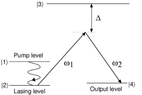
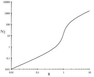
Figure 2: Schematic level diagram for the atom laser model of Moy et al.[36] (left). Plot of the steady state number of atoms in the lasing mode, as a function of the dimensionless pumping rate, $R$ (right). Threshold occurs at $R=1$.

The resulting rate equations for the numbers of atoms $N_{k}$ in level $|k\rangle$ are

$$\frac{dN_{1}}{dt} = r_{1}-\sum_{j}g_{j}(N_{2j}+1)r_{12}N_{1}-(1-\sum_{j}g_{j})r_{12}N_{1},$$

$$\frac{dN_{2j}}{dt} = g_{j}r_{12}N_{1}(N_{2j}+1)-r_{24}N_{2j}+~{}G_{j}(N_{2j}+1)N_{4}r_{24},$$

$$\frac{dN_{4}}{dt} = \sum_{j}N_{2j}r_{24}-\sum_{j}G_{j}(N_{2j}+1)N_{4}r_{24}-N_{4}\frac{1}{t_{0}}.$$ (24)

The $N_{2j}$ are the numbers of atoms in level $|2\rangle$ in the $j$th mode of the lasing level trap. $g_{j}$ is the overlap between the pump mode and the $j$th mode of the lasing trap. $G_{j}=N_{4j}/N_{4}$ is the proportion of atoms with electronic level $|4\rangle$ that have the same spatial mode as the $j$th mode of the lasing trap. $t_{0}$ is the time scale on which atoms are irreversibly lost from the system due to the Raman momentum kick. For a more complete description of these equations refer to Moy et al.[36].

The solutions of these rate equations show behaviour familiar from optical lasers. The steady state population of the laser mode $N_{21}$ as a function of a suitably scaled pump rate $R=r_{1}g_{1}/r_{24}$ shows a rapid increase at the threshold value of $R=1$, as shown in Fig. 2. As a function of time the above threshold values of the lasing cavity mode populations $N_{2j}$ show initial growth, and then all but the lasing mode $N_{21}$ decay. This is the familiar mode competition in which the “winner takes all” due to runaway Bose stimulation.

The rate equation model of Olshanii et al.[4] is similar in form. However they included photon reabsorption and found that lasing is inhibited by small amounts of reabsorption.

5.2 Mean-field models

In this approach, the atom laser is modelled using the Gross-Pitaevskii (GP) type equations discussed in section 3. The “mean-field” is the GP wavefunction which determines the effective potential felt by an atom due to its 2-body interactions with all of the other atoms in the condensate. Indeed one of the advantages of GP models is this straightforward treatment of atom-atom interactions.

Kneer et al.[42] describe a GP model of an atom laser including pump and loss terms. The modified GP equation for the laser mode macroscopic wavefunction is

$$i\hbar\frac{\partial\psi}{\partial t}=-\frac{\hbar^{2}}{2m}\frac{\partial^{2}\psi}{\partial x^{2}}+V_{E}(r)\psi+U_{0}|\psi|^{2}\psi~{}+H_{\mbox{\small gain}}\psi+H_{\mbox{\small loss}}\psi.$$ (25)

The first three terms are standard. The gain and loss are represented by phenomenological terms with rate constants $\Gamma$ and $\gamma_{c}$ respectively,

$$H_{\mbox{\small gain}}\psi=\frac{i\hbar}{2}\Gamma N_{u}\psi,\quad H_{\mbox{\small loss}}\psi=-\frac{i\hbar}{2}\gamma_{c}\psi.$$ (26)

In addition to the GP equation (25), a rate equation is used to describe the number of uncondensed atoms, $N_{u}$,

$$\frac{dN_{u}}{dt} = R_{u}-\gamma_{u}N_{u}-\Gamma N_{c}N_{u}.$$ (27)

$R_{u}$ describes a source which pumps the uncondensed state at rate $R_{u}$. The term $\gamma_{u}N_{u}$ describes atoms lost from the system, but not trapped in the condensed state. The final term describes the transfer of atoms into the condensed state. The condensate loss is spatially homogeneous, and undamped collective excitations are found. To avoid this they introduce a spatially dependent decay rate, so that $\gamma_{c}$ is a function of position, $\gamma_{c}(x)$. This produces a single lasing mode as the spatially dependent loss leads to mode selection.

Robins et al.[43] present a GP model which combines the pumping model of Kneer et al., with an explicit treatment of the output coupling and of the output beam. Including the output beam in the model allows one to investigate its spectrum and spatial distribution. Furthermore, non-Markovian effects in the output, such as Rabi oscillations between the condensate and beam, can be explored. The equations which describe the laser mode $\psi^{a}(x,t)$, and the output beam $\psi^{b}(x,t)$ are

$$i\hbar\frac{\partial\psi^{a}}{\partial t} = -\frac{\hbar^{2}}{2m}\frac{\partial^{2}}{\partial x^{2}}\psi^{a}+\frac{1}{2}m\omega^{2}x^{2}\psi^{a}+U^{a}_{0}|\psi^{a}|^{2}\psi^{a}+U^{a}_{0}|\psi^{b}|^{2}\psi^{a}$$

$$-i\gamma_{r}(|\psi^{a}|^{4}+|\psi^{b}|^{4})\psi^{a}-\hbar\Gamma_{R}e^{ik_{0}x}\psi^{b}(x)+\frac{i\hbar}{2}~{}\Gamma~{}N_{u}\psi^{a},$$

$$i\hbar\frac{\partial\psi^{b}}{\partial t} = -\frac{\hbar^{2}}{2m}\frac{\partial^{2}}{\partial x^{2}}\psi^{b}+mgx\psi^{b}+U^{b}_{0}|\psi^{b}|^{2}\psi^{b}+U^{a}_{0}|\psi^{a}|^{2}\psi^{b}$$ (28)

$$-i\gamma_{r}(|\psi^{a}|^{4}+|\psi^{b}|^{4})\psi^{b}-\hbar\Gamma_{R}e^{-ik_{0}x}\psi^{a}.$$

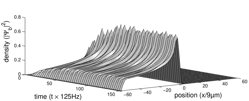
Figure 3: Atom laser beam density as a function of position and time, showing a quasi-steady state. Atoms are absorbed at the spatial boundaries. Parameters are given by Robins et al.[43].

The number of uncondensed atoms $N_{u}$ obeys Eq.(27). The Raman output coupling is described by the terms containing the momentum kick generators $e^{\pm ik_{0}x}$. Three body recombination has been included as a condensate loss mechanism, by the terms proportional to $\gamma_{r}$. This is found to have a stabilising effect on the non-linear dynamics of the atom laser. Two-body losses have not been included.

Typical output from a one dimensional numerical solution of this model is shown in Fig. 3. The oscillations represent nonlinear dynamical noise, which will determine the laser’s effective linewidth, or first order coherence. This is an example of physics which cannot be treated by the rate equation approach.

How mean field models may be extended to incorporate finite temperature effects, such as the population of excited levels, is described in subsequent sections, and by Burnett and Griffin in this volume.

5.3 Fully quantum mechanical models

A number of quantum optical master equation based models of the atom laser have been discussed in the literature[6, 37, 38, 39]. The model of Holland et al.[6] is based on evaporative cooling and incorporates: the creation of an atom in the trap from the pump field, the loss of an atom from a high lying trap state, collisions which scatter atoms into or out of the ground state, and the loss of atoms from the ground state through output coupling.

A three level model is sufficient to describe these features. Atoms are injected with rate $\kappa_{1}$ in level one and are lost with rates $\kappa_{0}$ and $\kappa_{2}$ from level zero and level two respectively. Only the energy conserving 2-body interaction terms are considered. Level two is adiabatically eliminated by assuming large damping due to the evaporative cooling. This leads to the master equation for the density operator $\rho$,

$$\frac{\partial\rho}{\partial t} = \frac{1}{i\hbar}\left[V_{i},\rho\right]~{}+\kappa_{0}\mathcal{D}[a_{i}]\rho+\kappa_{1}\mathcal{D}[a_{i}^{{\dagger}}]\rho+\Omega_{r}\mathcal{D}[a_{0}^{{\dagger}}a_{1}^{2}]\rho$$ (29)

where

$$V_{i}=\hbar(a_{0}^{{\dagger}}a_{0}-2n_{0})(V_{0000}a_{0}^{{\dagger}}a_{0}+V_{0101}a_{1}^{{\dagger}}a_{1})+\hbar V_{1111}a_{1}^{{\dagger}2}a_{1}^{2},$$ (30)

and $n_{0}$ is the mean population of level zero. The loss terms are assumed to be of the standard (Born-Markovian) Lindblad form, defined by

$$\mathcal{D}[c]\rho=2c\rho c^{{\dagger}}-(c^{{\dagger}}c\rho+\rho c^{{\dagger}}c)$$ (31)

The effective redistribution rate $\Omega_{r}$ is proportional to $|V_{0211}|^{2}/\kappa_{2}$.

Equations for the populations, $\langle nk|\rho(t)|nk\rangle$, where $|nk\rangle$ describes a state with $n$ atoms in level zero and $k=0$ or $k=1$ atoms in level one, are obtained. Level one is rapidly depleted by two atoms scattering into levels zero and two. The steady state population of the level zero lasing level is found to be Poissonian with mean atom number $2\kappa_{1}/(3\kappa_{0})$. Thus when loss out of the lasing mode is sufficiently small $\kappa_{0}<<\kappa_{1}$, a large population can build up in the lasing mode.

In order to produce a state with a well defined phase they consider parameter regimes where $\Omega_{r}$ is much larger than the frequency shifts in $V_{i}$. This inhibits the dispersive nature of the latter from destroying phase coherence. They find that, as for an optical laser, line narrowing occurs as the population of the ground state increases. However, in a refinement of the model due to Wiseman et al.[39] the linewidth of the laser output is broader than the bare linewidth of the laser mode.

The crucial refinement is in the description of the pumping of level 1. The approximation that Holland et al. make allows atoms to leak into, but not out of, the trap. To allow the latter Wiseman et al. replace the term $\kappa_{1}\mathcal{D}[a_{1}^{{\dagger}}]\rho$ with

$$\kappa_{1}(N+1)\mathcal{D}[a_{1}^{{\dagger}}]\rho+\kappa_{1}N\mathcal{D}[a_{1}]\rho.$$ (32)

The $N$ is the mean population of the pump reservoir modes. In fact, there is no limit in which the extra terms can be ignored. When $\kappa_{0}<<\kappa_{1}$, there are two distinct parameter regimes depending on the relative size of a parameter proportional to $\kappa_{2}|V_{0211}|^{2}$, which they call $\Gamma$, and $\kappa_{0}$. These they call the strong and weak collision regimes: $\Gamma>>\kappa_{0}$ and $\Gamma<<\kappa_{0}$ respectively. In the weak collision regime, $\Gamma<<\kappa_{0}$ there is a large population in the laser mode if $N>>1$, i.e. with strong pumping. The power spectrum reveals a linewidth larger than the bare linewidth of the lasing mode. Nevertheless, the phase diffusion rate may still be slow in the sense of being much less than the output flux of atoms from the lasing mode.

Wiseman and Collett[44] proposed an atom laser model using optical dark state cooling. The laser is found to have a linewidth narrower than the bare linewidth. This is an improvement on models based on evaporative cooling discussed above. The output is also found to be second order coherent.

The master equation is one means of describing the full quantum statistics of an atom laser. It has the great advantage of drawing on the wealth of techniques that have been developed in quantum optics[25]. However, a fully quantum theory of the atom laser can be developed without using the standard master equation approximations[45, 46, 47]. In particular, assuming a Born-Markov form for the output coupling ignores the possibility of the output beam acting back on the laser mode. This may happen, for example, due to Rabi cycling between the output and laser modes.

Hope[45] developed a general theory of the input and output of atoms from an atomic trap. Moy et al.[46] used this theory to find an analytic expression for the spectrum of a beam of atoms output from a single mode atomic cavity. For very strong coupling it is just the spectrum of the trapped lasing mode, and is therefore broad. As the strength of the coupling is reduced, the linewidth is reduced. For small coupling strengths the lineshape approaches a Lorentzian, centred about the energy of the cavity with a linewidth proportional to the coupling strength. Hope et al.[47] include a pumping mechanism and they find that the output spectrum is substantially wider than that obtained using the Born-Markov approximation. However an important limitation of these theories is that they do not include 2-body interactions.

6 Atomic Gain

We have seen in sections 1 and 5 that a mechanism for atomic gain, to provide coherent amplification of the atomic field in the lasing mode, is an essential element of an atom laser. A number of gain mechanisms have been proposed, (e.g. see section 5.1) but to date only one, evaporative cooling, has been demonstrated experimentally. The process of evaporative cooling is based on the removal of high energy atoms from the gas, so that subsequent collisional rethermalisation of the remaining atoms results in a distribution of lower temperature (i.e. lower average energy). Under appropriate conditions, bosonic stimulation of transitions into the ground state of the confining potential leads to the formation of a Bose condensate: in an atom laser this would constitute the lasing mode.

The kinetics of condensate growth has long been a subject of theoretical study^47-49, but the first quantitative calculations were carried out only recently by Gardiner. Together with coworkers he has given a comprehensive treatment of condensate formation by bosonic stimulation, in a series of papers^50-55. In this section we review the major features and results of this theory.

6.1 Quantum Kinetic theory

The starting point of the treatment is the third in a series of papers on Quantum Kinetic theory developed by Gardiner and Zoller[53], which we shall refer to as QKIII. We note that an alternative formulation of a Quantum Kinetic theory has been given by Griffin and coworkers (see this volume, and references therein). The gas of Bose atoms in a harmonic trap of frequency $\omega$ is described by a second-quantized field, as in Eqs.(1 - 4). Two-body collisions are included but three-body collisions are neglected. Guided by the fact that the energy spectrum above a certain value $E_{R}$ is unaffected by the presence of the condensate, we can divide the field into the condensate band (all energy levels below $E_{R}$) and the non-condensate band (all the energy levels above $E_{R}$), as represented in Fig. 4.

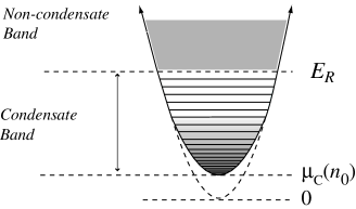
Figure 4: Schematic representation of modification of trap energy levels by condensate meanfield. Levels above $E_{R}$ are unaffected.

The noncondensate band (which contains the majority of the atoms) is taken to be fully thermalised, in the sense that for any point $\mathbf{r,k}$ in phase space the single particle distribution function $F(\mathbf{r,k})$ (in principle a Wigner function) is localised, and has a well defined temperature $T$ and chemical potential $\mu$. Thus the noncondensate band can be treated as a time independent bath, and a master equation is derived for the density matrix of the condensate band, (Eqs. (50a)-(50f) QKIII). It is worth emphasizing that in general the condensate band is not in thermal equilibrium, and the master equation provides a description of its dynamical evolution. The level structure of the condensate band is well described by the Bogoliubov spectrum, and Gardiner[58] has shown that appropriate states for this band are $|N,\{n_{m}\}\rangle$ which have a definite number $N$ of total particles in the band, and a set of numbers $\{n_{m}\}$ representing the occupation numbers of the condensate ($m=0$) and quasiparticle (excited Bogoliubov) levels. In this treatment, the condensate wavefunction and energy eigenvalue (the condensate chemical potential $\mu_{C}(N)$ ) are given by the time-independent Gross-Pitaevskii equation with $n_{0}$ atoms. The quasiparticles may be particle-like excitations (at higher energies) or phonon-like collective excitations (at low energies). The phonon excitations are not eigenstates of the number operator and thus the total population of the quasiparticles need not be conserved, in contrast to $N\;$which is strictly conserved.

By taking a representation of the master equation in terms of the states $|N,\{n_{m}\}\rangle$, and then taking the diagonal elements, a stochastic master equation for the occupation probabilities $p(N,\{n_{m}\})$ is obtained. The transitions appearing in this equation can be divided into those which change the number of atoms $N$ in the condensate band, and those which do not. The former, which we call growth processes, arise predominantly from collisions of two noncondensate atoms where one of the outgoing atoms goes into the condensate band. The reverse collision is also included in the growth processes. The transitions which do not change $N$ are called scattering processes, and arise predominantly from collisions between a condensate band atom and a noncondensate band atom which leave one atom in each band. Other collision processes, in which the pair of colliding atoms either begins or ends in the condensate band, will in principle also contribute to growth or scattering, but can be neglected since the condensate band contains such a small fraction of all the atoms. We note that collisions between pairs of atoms that begin and remain in the noncondensate band play the role of thermalising the bath and do not appear in this master equation.

6.2 ‘Particle-like’ rate equations

Using standard methods, a deterministic rate equation for the mean population $\langle n_{m}\rangle$ of the $m$th quasiparticle level (which we will subsequently write $n_{m}$) can be obtained from the master equation and we write it as

$$\frac{dn_{m}}{dt}=\dot{n}_{m}|_{\mathrm{growth}}+\dot{n}_{m}|_{\mathrm{scatt}}$$ (33)

where the forms for the growth transition rates $\dot{n}_{m}|_{\mathrm{growth}}$ and the scattering transition rates $\dot{n}_{m}|_{\mathrm{scatt}}$ will be discussed below. A similar deterministic rate equation can be written for the mean population of the condensate band $\langle N\rangle$ (which we will subsequently write $N$).

The growth transition rates $\dot{n}_{m}|_{\mathrm{growth}}$ can be obtained in explicit form from the population master equation given in Eq.(189) QKIII, and comprise all the processes where $N\;$changes by $1,$ and one of the quasiparticle populations, $n_{j}$ say, changes by $1$ or $0,$ (with all other $n_{k}$ unchanged). Most of these processes (e.g. $N$ $\rightarrow N+1$ and $n_{j}\rightarrow n_{j}+1,$ or $N$ $\rightarrow N+1$ and $\{n_{m}\}$ unchanged) admit a particle-like interpretation. However, those processes where $N$ and $n_{j}$ change in opposite directions have to be interpreted as phonon-like processes, and for example could represent a process where the condensate is initially oscillating, and a thermal atom is added to the condensate band and causes the condensate oscillation to be reduced. All such phonon-like processes are neglected in this treatment, since only a small fraction of quasiparticle wavefunctions have phonon-like character, and we expect they will play an unimportant part in the condensate growth. The growth terms for the quasiparticle levels thus simplify to the form

$$\dot{n}_{m}|_{\mathrm{growth}}=2W_{m}^{++}(N)\left(n_{m}+1\right)-2W_{m}^{--}(N)n_{m}$$ (34)

and the equation for the mean number in the condensate band becomes

$$\frac{dN}{dt}=2W^{+}(N)\left(N+1\right)-2W^{-}(N)N$$ (35)

where $W_{m}^{++}(N)$ and $W^{+}(N)$ are forward rates and $W_{m}^{--}(N)$ and $W^{-}(N)$ are backward rates. It is shown in QKIII that when the condensate wavefunction $\xi_{N}(\mathbf{r})$ is sharply peaked compared to the spatial dependence of $F(\mathbf{r,k}),$ then

$$W^{+}(N) = {\frac{4a^{2}}{m^{2}(2\pi)^{3}}}\int d^{3}\mathbf{K}_{1}\int d^{3}\mathbf{K}_{2}\int d^{3}\mathbf{K}_{3}\int d^{3}\mathbf{k}\,\delta(\mathbf{K}_{1}+\mathbf{K}_{2}-\mathbf{K}_{3}-\mathbf{k})$$ (36)

$$\!\!\!\!\!\!\!\delta(\Delta\omega_{123}-\mu_{C}(N)/\hbar)F(0\mathbf{,K}_{1})F(0\mathbf{,K}_{2})\left(1+F(0\mathbf{,K}_{3})\right)|\tilde{\xi}_{N}(\mathbf{k})|^{2}$$

The integrand represents a collision in which a pair of noncondensate atoms of momenta $\mathbf{K}_{1}$ and $\mathbf{K}_{2}$ produces one noncondensate atom ($\mathbf{K}_{3}$) and one condensate band atom of momentum $\mathbf{k}$. Energy conservation is expressed in the second $\delta$ function, in which $\Delta\omega_{123}=\omega_{\mathbf{K}_{1}}+\omega_{\mathbf{K}_{2}}-\omega_{\mathbf{K}_{3}},$ where $\hbar\omega_{\mathbf{K}_{i}}=$ $\hbar^{2}\mathbf{K}_{i}^{2}/2m$ $+V_{T}(0)$ is the particle energy at the centre of the trap potential $V_{T}$. $\tilde{\xi}_{N}(\mathbf{k})$ is the momentum-space ground-state wavefunction. The expression for $W_{m}^{++}(N)$ is similar to Eq.(36), and the forward and backward rates are related by

$$W^{+}(N) = e^{[\mu-\mu_{C}(N)]/kT}W^{-}(N)$$ (37)

$$W_{m}^{++}(N) = e^{[\mu-e_{m}]/kT}W_{m}^{--}(N)$$ (38)

where $e_{m}$ is the energy of the $m^{th}$ quasiparticle level. Equations (33)-(38) are derived within the approximation that the number of particles in the condensate, $n_{0},$ is large enough that we can write $n_{0}\approx N,($which is required for the Bogoliubov spectrum to be accurate). However, in the early stages of condensate growth when $n_{0}$ is small, the unperturbed spectrum should be used, and will be accurate provided none of the condensate band levels are too highly populated. This means that by making the replacement $N\rightarrow n_{0}$ in Eqs.(33)-(38) those equations will provide a good description of the dynamical evolution of the levels in the condensate band throughout the formation of the condensate. Values for the rates $W^{+}$ can be obtained in varying levels of approximation, and the simplest expression, used in the first quantitative description of growth[52], is obtained by assuming a classical Maxwell-Boltzmann distribution for $F(\mathbf{r,k}),$ and allowing the integrals in $\mathbf{K}_{1,2,3}$ in Eq.(36) to extend over all energies, rather than just the noncondensate band. This leads to the explicit expression

$$W^{+}(n_{0})\approx{\frac{4m(akT)^{2}}{\pi\hbar^{3}}}e^{2\mu/kT}$$ (39)

in which we note the prefactor to the exponential is independent of $n_{0}$ and is essentially the elastic collision rate $\rho\sigma v$ with quantities evaluated at the critical point for condensation. More accurate evaluations[54, 56] of $W^{+}$ which take into account the Bose-Einstein nature of the non-condensate distribution and exclude the condensate region in the $\mathbf{K}$ integrals, give a value about three times larger than that of Eq.(39). $W_{m}^{++}(n_{0}),$ which has a form similar to Eq.(36), is more difficult to evaluate but is of the same order of magnitude as $W^{+}(n_{0}),$ and in the first instance we set $W_{m}^{++}(n_{0})\approx W^{+}(n_{0}).$ The sensitivity of the results to this approximation will be discussed in section 6.3. Finally, in order to reduce the number of equations to a tractable set, an ergodic assumption is made which allows us to group together levels of similar energy into small sub-bands, with only the ground state being described by a single level. The sub-bands have (central) energy $e_{m}$ and degeneracy $g_{m}$, and the equations for the growth processes of these bands are

$$\dot{n}_{m}|_{\mathrm{growth}} = 2W_{m}^{++}(n_{0})\left\{\left[1-e^{[e_{m}-\mu]/kT}\right]n_{m}+g_{m}\right\},$$ (40)

$$\dot{n}_{0}|_{\mathrm{growth}} = 2W^{+}(n_{0})\left\{\left[1-e^{[\mu_{C}(n_{0})-\mu]/kT}\right]n_{0}+1\right\}.$$ (41)

These equations exhibit the most important features of condensate growth, or atomic gain, as we shall discuss shortly in section 6.3. The remaining terms required for Eq.(33), the scattering terms $\dot{n}_{m}|_{\mathrm{scatt}}$, describe processes in which a condensate band atom and a noncondensate band atom collide and leave one atom in each band. Gardiner and Lee[56] have evaluated the scattering terms within well defined approximations (for the case of an isotropic trap), to give

$$\dot{n}_{m}|_{\mathrm{scatt}}={\frac{8ma^{2}\omega^{2}}{\pi\hbar}}e^{\mu/k_{B}T}\Gamma(T)\times$$

$$\,\,\Bigg{\{}\sum_{k<m}{\frac{1}{g_{m}}}\left[n_{k}(g_{m}+n_{m}){e^{-\hbar\omega_{mk}/k_{B}T}}-n_{m}(g_{k}+n_{k})\right]$$

$$\,\,+\sum_{k>m}{\frac{1}{g_{k}}}\left[n_{k}(g_{m}+n_{m})-n_{m}(g_{k}+n_{k}){e^{-\hbar\omega_{km}/k_{B}T}}\right]\Bigg{\}}.$$ (42)

where $\Gamma(T)=\sum_{e_{m}>E_{R}}e^{-e_{m}/kT}$ , $\hbar\omega_{nq}=e_{n}-e_{q}$, and the notation $k>m$ means $e_{k}>e_{m}$.

6.3 Results

Equations (40 - 42) provide an explicit form for the set of deterministic rate equations for populations in the condensate band, with the size of the set determined by the amount of level grouping. Much of the behaviour that occurs in the full set of equations is captured by a simple implementation in which the condensate band is represented by only one level[52], i.e. the condensate. The equations then reduce to a single equation (41), which has the laser-like features of stimulated transition rates (the terms proportional to $n_{0}$) and a spontaneous transition rate (the term +1 in the curly braces) which initiates growth. In addition, this so-called simple growth equation has thermodynamic features, in that the forward and backward transition rates become equal (i.e. equilibrium is reached) when the chemical potential of the condensate, $\mu_{C}(n_{0}),$ becomes equal to $\mu$ of the thermal bath (to order $1/N$). A crucial aspect of the growth process is that as the condensate grows, the meanfield causes $\mu_{C}(n_{0})$ to increase, beginning from $\mu_{C}(0)=$ $3\hbar\omega/2$ (the trap zero-point energy), and rising as $\left(n_{0}\right)^{2/5}$ (in the Thomas-Fermi approximation) at large $n_{0}$. It is clear that a condensate can only grow if the thermal bath has $\mu>0,$ and this is achieved in the process of evaporative cooling by removing the highest energy atoms. The higher energy levels quickly come to their equilibrium distributions, but the lower energy levels remain far from equilibrium, and the ensuing tendency of collisions of lower energy bath atoms to feed the condensate band can be characterised by a bath chemical potential $\mu>0.$

A typical result for the simple growth equation is shown as the dotted line in Fig.5

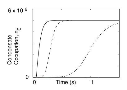
Figure 5: Typical condensate growth curves for different implementations of the model: simple growth equation (dotted line); full model (solid line); with no scattering (dashed line). Parameters are appropriate to the regime of the MIT experiment: $\mu=43.3\hbar\omega$, $T=900$ nK, $n_{0}(t=0)=100.$

where we have chosen a case corresponding to the conditions of the MIT growth experiment[57] in which sodium atoms of scattering length $a=2.75$ nm are contained in a trap of geometrical mean frequency $\omega=2\pi\times 50$ Hz. Although we do not expect quantitative accuracy from this simple model, the characteristic S shape of the growth curve exhibits the key aspects of the growth process. In the initial stages the growth is slow and arises from spontaneous transitions; then as $n_{0}$ increases, stimulated transitions dominate and the growth is steep. Finally, as the condensate chemical potential approaches $\mu,$ there is a slow approach to equilibrium.

Of course for a quantitatively accurate treatment, more condensate band levels must be included, along with the more careful calculation for $W^{+}$ (see Eq.(10) ref[54]). Typically 20-50 sub-bands are used, each of width $\approx$ $\hbar\omega.$ The energy $e_{m}$ of these sub-bands increase as $n_{0}$ grows, with the lower levels most affected, and the levels at the top of the condensate band not affected at all. Although the increase of the condensate energy level is crucial to the growth process and must be treated as accurately as possible, it is found that there is little sensitivity to the scheme used to alter the quasiparticle energy levels. Typically, the levels between $\mu_{C}(n_{0})$ and $2\mu_{C}(n_{0})$ are compressed from the bottom in a linear fashion, and higher levels are unaltered. The solid line in Fig.5 shows the effect of using a set of sub-bands in the growth process. The physical parameters are identical to those used in the simple growth model (the dotted curve) but there has been a speed up of about an order of magnitude. The effects of the scattering terms can be separated from the growth terms, as we show with the dashed line in Fig.5, which is a calculation using the same number of sub-bands as for the solid curve, but with all scattering terms put to zero. It is clear that the main effect of the scattering processes is to cause the initiation of condensate growth to occur much more sharply. This is due to the fact that the growth processes can initially populate a wide number of sub-bands, and then scattering allows these populations to be redistributed directly into the condensate. The steep part of the growth curve is essentially unchanged by scattering, since it is dominated by the stimulated terms in the growth processes.

A number of sensitivity studies were carried out by Gardiner and Lee[56], who showed that the scattering transition rates could be varied by two orders of magnitude, the relative size of $W^{++}$ to $W^{+}$ could be varied by a factor of 2, and a wide variety of initial conditions for the rate equations could be used, with only moderate effects on the growth curves.

6.4 Full dynamical solution

The master equation approach described above, which assumes a nondepletable bath of fixed thermodynamic properties, can be expected to be inaccurate when high fraction condensates form. Under those circumstances the full dynamics of the system must be considered, and Davis et al. [59] have treated this problem using a modified Quantum Boltzmann formulation. In their treatment the single particle distribution function $f_{n}$ for the $n^{th}$ energy sub-band evolves according to

$$g_{n}\frac{\partial f_{n}}{\partial t} = \frac{8ma^{2}\omega^{2}}{\pi\hbar}\sum_{p,q,r}\delta_{e_{r}+e_{n},e_{p}+e_{q}}g_{\min(p,q,r,n)}$$ (43)

$$\times\left\{f_{p}f_{q}\left(1+f_{r}\right)\left(1+f_{n}\right)-\left(1+f_{p}\right)\left(1+f_{q}\right)f_{r}f_{n}\right\}.$$

This equation appears similar to the ergodic form of the well-known Quantum Boltzmann equation (e.g. see ref [60]) but the crucial modification from Quantum Kinetic theory is that the energy levels $e_{m}$ and the degeneracies $g_{m}$ alter as the condensate population changes. A division of the levels into condensate and noncondensate bands is now made only for computational purposes, and the evolution of all sub-band levels is explicitly followed. In addition to the collisional processes treated in the master equation method, Eq.(43) includes thermal scattering processes where the pair of colliding atoms begin and remain in the noncondensate band, as well as collisions which either begin or end with a pair of atoms in the condensate band. As before, all levels are treated as particle-like, which allows an analytic expression to be obtained for the density of states and its dependence on the condensate occupation. The numerical simulation of Eq.(43), which we shall refer to as the full dynamical solution, requires vastly more computation than the rate equation model described in section 6.2, and considerable care must be taken with ensuring energy conservation in the collisional calculations and in rebinning the sub-bands at each time step. Details are given in ref [59].

For small condensate fractions (of less than about 10%) the full dynamical solution agrees well with the rate equation solution. However for larger fractions, as illustrated in Fig. 6(a)

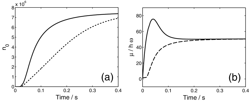
Figure 6: (a) Comparison of condensate growth models for a final condensate fraction of 24%. Solid line, simulation of Eq.(43) [with $\mu=0$ before evaporative cut]. Dotted line, rate equation model. Final condensate parameters $n_{0}=7.5\times 10^{6},T=590$nK. (b) Chemical potentials $\mu_{\mathrm{eff}}$ (solid line) and $\mu_{C}(n_{0})$ (dashed line).

we find that the bath dynamics have an appreciable effect. For this case, where parameters are chosen to be appropriate for the MIT experiment and the final condensate fraction is 24%, the full dynamical solution (solid line) grows faster than the rate equation solution (dotted line). This can be most easily understood by introducing the concept of an effective chemical potential $\mu_{\mathrm{eff}}$ for the thermal cloud (obtained by fitting a Bose-Einstein distribution to the distribution function above $E_{R})$ and using this in the simple growth equation Eq.(41). Figure 6(b) shows the evolution of both $\mu_{\mathrm{eff}}$ and $\mu_{C}(n_{0})$ during the simulation, and we can see that during the stimulation-dominated period of growth, $\mu_{\mathrm{eff}}$ substantially exceeds the final equilibrium value, and thus from Eq.(41), the backward rate from condensate to thermal cloud is greatly inhibited. Ultimately this is due to the very severe cut that is required on the initial equilibrium distribution in order to allow evaporative cooling to proceed to such a high condensate fraction. We note that Zaremba et al.[61] have treated the full dynamical problem using a somewhat different formalism, but obtain essentially the same numerical results.

The theory reviewed in this section can be compared to the experimental results of the MIT group[57]. It is found [54, 56, 59] that there is very good agreement in some parameter regimes, but significant discrepancies in others, which may be attributable to the difficulty of fully characterising the experimental parameters. A definitive comparison is handicapped by the unavailability of a wide range of primary experimental data, and further experiments will be required to comprehensively test the theoretical predictions.

7 Output Coupling

An output coupler for an atom laser is a device which extracts atoms from the laser mode while preserving their coherence. All current coupler mechanisms are based on applying an electromagnetic field to change the internal state of the atom from a trapped to an untrapped state[2]. The first demonstration of an atom laser, by the MIT group[62], used an RF pulse to transfer atoms into untrapped zeeman substates, where they then fell freely under gravity. A refinement of this technique, using a precisely controlled trap and cw-RF fields has been used to produce a quasi-cw coherent output beam[63]. The use of Raman coupled output fields offers some advantages, principally in providing a momentum kick to the outgoing atom beam[46], but also in that the optical fields can be focussed into a small volume, achieving a measure of spatial selectivity for the coupling. Recently the NIST group[17] demonstrated Raman output coupling in an experiment where the output beam was ejected in the horizontal direction.

A number of mean field theoretical treatments have been given of RF[40, 64] and Raman couplers[66], and elsewhere[65] the effects of gravity have been included. Recently the Oxford group[67, 68], have given a detailed treatment of output coupling from a finite temperature condensate. In this section we review the theory of output couplers, beginning with a mean field treatment, which establishes a framework for both RF and Raman output couplers. We then briefly summarize the theory of finite temperature couplers.

7.1 Mean field treatment of output coupling

The basis of the mean field treatment of an output coupler is a pair of coupled GP equations for the mean fields $\psi_{1}$ and $\psi_{2}$ of atoms in internal states $|1\rangle$ and $|2\rangle$, as discussed previously in section 5.2. For convenience, we present a dimensionless form of the equations

$$\frac{\partial\psi_{1}}{\partial t}\! = \!i\nabla^{2}\psi_{1}\!-\!iV_{1}\psi_{1}\!+\!i\frac{\lambda^{\ast}(\mathbf{r},t)}{2}\psi_{2}\!-\!iC\!\left[|\psi_{1}|^{2}\!+\!w|\psi_{2}|^{2}\right]\!\psi_{1}\!-\!iGy\psi_{1},$$ (44)

$$\frac{\partial\psi_{2}}{\partial t}\! = \!i\nabla^{2}\psi_{2}\!-\!iV_{2}\psi_{2}\!+\!i\frac{\lambda(\mathbf{r},t)}{2}\psi_{1}\!\!-\!iC\!\left[|\psi_{2}|^{2}\!+\!w|\psi_{1}|^{2}\right]\!\psi_{2}\!-\!iGy\psi_{2}\;.$$ (45)

We shall assume that state $|1\rangle$ is the trapped state, with a harmonic potential $V_{1}$ while state $|2\rangle$ is untrapped ($V_{2}=0$) or anti-trapped ($V_{2}=-V_{1}$), so that $\psi_{2}$ represents the output field. In Eqs.(44) and (45) the units of time ($\tilde{t}_{0}$) and distance ($\tilde{x}_{0}$) are respectively $\omega^{-1}$ and $(\hbar/2m\omega)^{1/2}$ where $\omega$ is the trap frequency, and the fields are normalised such that $\int\!\left[|\psi_{1}|^{2}\!+\!|\psi_{2}|^{2}\right]d^{3}r=1$. The nonlinearity constant $C$ is $4\pi\hbar aN/(m\omega\tilde{x}_{0}^{3})$ (in 3D), and the relative scattering length $w$ of the inter- to intra-species collisions is typically close to 1. Gravity acts in the $-y$ direction, and the scaled acceleration is $G=mg\tilde{x}_{0}/\hbar\omega.$ The coupling term $\lambda$ can describe either a single photon coupling or a two photon (Raman) coupling, and can be written in terms of a slowly varying envelope $\Omega(\mathbf{r},t)$

$$\lambda(\mathbf{r},t)=\Omega(\mathbf{r},t)\exp i(\mathbf{k}_{em}\cdot\mathbf{r-}\Delta_{em}t)$$ (46)

where $\mathbf{k}_{em}$ and $\Delta_{em}$ measure the net momentum and net energy transfer from the EM field to the output atom (in units $\hbar/\tilde{x}_{0}$ and $\hbar\omega$ respectively). For the case of a single photon transition, $\Delta_{em}=\omega_{1}-\omega_{21},$ where $\omega_{1}$ is the photon frequency, $\omega_{21}$ is the energy difference $E_{2}-E_{1}$ between states $|2\rangle$ and $|1\rangle$ (in the absence of the traps), and $\Omega(\mathbf{r},t)$ is the Rabi frequency. For a Raman transition connecting $|1\rangle$ to $|2\rangle$ (through a far detuned intermediate state) via the absorption of a photon $\omega_{1}$ and the emission of photon $\omega_{2}$ then $\Delta_{em}=\omega_{1}-\omega_{2}-\omega_{21},$ and $\Omega(\mathbf{r},t)$ is equal to $\Omega_{2}^{\ast}\Omega_{1}/\Delta$ where $\Omega_{j}$ is the Rabi frequency associated with the $\omega_{j}$ radiation field, and $\Delta$ is the detuning from the intermediate state. Our main interest here is in cw coupling, and so $\Omega(\mathbf{r},t)$ will be independent of time. The key difference between RF coupling and Raman coupling is that for RF coupling, the momentum $\mathbf{k}_{em}$ is negligible and can be ignored. Typically RF coupling (which may extend into the microwave region) is single photon, but Raman coupling necessarily involves two photons. We note that in Eqs.(44) and (45) we have neglected the light shifts that would occur for the two photon case, under the assumption that they would be small compared to the potentials $V_{j}$ or the collisional mean fields near the trap.

The coupler equations (44) and (45) can be solved numerically, and we illustrate in Fig. 7 a case for an RF coupler in two dimensions, where the system begins in an eigenstate of the trap $V_{1}$, the RF field is plane wave, and $V_{2}=0.$

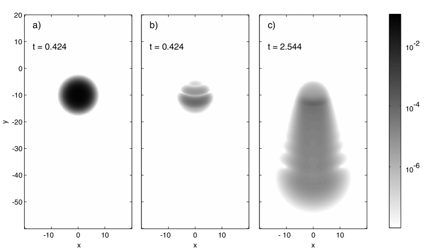
Figure 7: Population densities in states $|1\rangle$ and $|2\rangle$ under cw output coupling in a gravitational field. (a) state $|1\rangle$ at $t=0.424$; (b) state $|2\rangle$ at $t=0.424;$ (c) state $|2\rangle$ at $t=2.544.$ Densities are plotted logarithmically. RF field is plane wave and parameters are $\Omega=0.2,$ $\Delta_{em}=40,$ $G=5,$ $C=200,V_{2}=0.$

The first two frames show $|\psi_{1}|^{2}$ and $|\psi_{2}|^{2}$ soon after the coupler has been turned on, and we note that the trapped state is essentially unchanged from its initial state, while the output state (more or less) copies the initial state. After some time, the output beam streams downwards under gravity in a well directed uniform beam that resembles the experimental results of the Munich group[63].

7.2 Analytic treatments

Many of the features of the output coupler behaviour that are found in simulations of Eqs.(44) and (45) can be understood in terms of analytic approximations. The key parameters are the strength of the coupling field ($\Omega$), the net energy match with the output states, and the bandwidth of the coupling. When $\Omega$ is large (more precisely[40] $\Omega^{2}+\Delta^{2}\gg\mu(\mu+2|\Delta|)$, where $\mu$ is the chemical potential of the initial trapped state), it dominates the remaining terms in Eqs.(44) and (45), and the resulting behaviour is synchronous Rabi cycling where each part of the condensate oscillates between being fully in state $|1\rangle$ and fully in state $|2\rangle$, at frequency $\Omega.$ The atoms spend such short periods of time in the untrapped state, that they are unable to escape. On the other hand when $\Omega$ is small compared to $\mu$, other terms in Eqs.(44) and (45) become more significant, and the difference between the trap potentials becomes important. We can understand this by transforming Eqs.(44) and (45) into a rotating frame using $\tilde{\psi}_{2}=\psi_{2}\exp(i\Delta_{em}t),$ neglecting kinetic energy (because $t$ is small and the atoms do not have time to move), and then recognising that the equations simply become Rabi cycling with a spatially dependent effective detuning

$$\Delta_{\mathrm{eff}}(\mathbf{r)}=\Delta_{em}-(V_{1}-V_{2})\,.$$ (47)

The mean field contribution to $\Delta_{\mathrm{eff}}$ cancels (for $w=1$) because the atom feels the same mean field in either state $|1\rangle$ or $|2\rangle.$ Now, because the spectral width $\Omega$ of the Rabi cycling is small, significant transfer from $|1\rangle$ to $|2\rangle$ will only occur in a small spatial region near the value of $\mathbf{r}$ for which $\Delta_{\mathrm{eff}}(\mathbf{r)}=0.$ The resulting spatially selective output coupling can be seen in Fig. 7 (b) and (c), where the preferred region of coupling is a narrow crescent near $y=-10.$ The location of this region can be calculated by noting that the magnetic traps (i.e. $V_{1}$ and $V_{2}$) are centered on $x=0,y=0,$ and thus the condition $\Delta_{\mathrm{eff}}(\mathbf{r)}=0$ for a given choice of $\Delta_{em}$ is equivalent to selecting an equipotential line for the potential difference $V_{1}-V_{2},$ which is a circle centered on $x=0,y=0.$ Due to gravity, the equilibrium centre of mass position of condensate $\psi_{1}$ drops below the centre of the magnetic trap to a position where the spring force is equal to the gravitational force, as shown in Fig. 7(a). Thus the spatially selected region of coupling, where the trap equipotential intersects the trapped condensate, takes a crescent shape. Of course the coupling time $\tau_{c}$ must be long enough that transient broadening does not obscure the spatial selectivity.

7.3 Weak coupling regime

The weak coupling regime is of most interest for cw atom lasers, and perturbative solutions have been derived which describe key aspects of the output field behaviour[66, 67]. Following those treatments we make the assumption of an undepleted trapped state and a very dilute output state, which allows us to replace $\psi_{1}$ in Eq.(45) by its initial value $\psi_{1}(t=0)$ and to neglect the meanfield interaction of the output state with itself. Taking a Thomas-Fermi approximation for $\psi_{1}(t=0)$, Eq.(45) becomes a linear Schrodinger equation

$$\frac{\partial\psi_{2}}{\partial t}\!=-iH_{oc}\psi_{2}+\!i\frac{\lambda(\mathbf{r},t)}{2}\Psi_{TF}\exp(-i\mu t)\!\!,$$ (48)

where $H_{oc}=-\nabla^{2}+V_{oc}$ . The potential for the outcoupled wave is $V_{oc}=V_{2}+w(\mu-V_{1})+Gy$ and the final term in Eq.(48) is a source term in which the Thomas-Fermi wavefunction is $\Psi_{TF}=[\mu-V_{1}]^{1/2}.$ The eigenfunctions $\phi_{E}(\mathbf{r})$ of $H_{oc}$ provide a convenient basis for solving Eq.(48). Taking for simplicity the one dimensional case (and neglecting gravity) we obtain the solution

$$\psi_{2}(x,t)=i\int dE\left\{e^{i(B-E)t}\left[\frac{\sin Bt}{B}\right]\right\}\Lambda(E)\phi_{E}(x)\,,$$ (49)

where $B=[E-(\mu+\Delta_{em})]/2$ and

$$\Lambda(E)=\frac{1}{2}\int dx\phi_{E}^{\ast}(x)\Omega(x)\exp(ik_{em}x)\Psi_{TF}\,,$$ (50)

is the matrix element of the EM coupling amplitude between the output eigenfunction and the Thomas-Fermi trap state. Eq.(49) provides useful insight into the properties of the output field. The term in square brackets is a familiar factor from perturbation theory, and at small times the term in braces $\left\{{}\right\}\longrightarrow t$ so that $\psi_{2}(x,t)\approx it[\Omega(x)/2]\exp(ik_{em}x)\Psi_{TF}(x).$ Thus at early times the weak coupler produces an output field that is a copy of the initial trapped state, spatially masked by the EM field amplitude. At long times the term in square brackets $[\,]\longrightarrow 2\pi\delta(E-\mu-\Delta_{em})$ so that the output state becomes proportional to the eigenfunction $\phi_{E}(x)$

$$\psi_{2}(x,t)\approx i2\pi\exp(-iE)t\Lambda(E)\phi_{E}(x)$$ (51)

where $E$ conserves energy according to

$$E=\mu+\Delta_{em}\,,\,$$ (52)

and the function $\Lambda(E)$ plays the role of a spectral filter. The low energy cutoff of $\Lambda(E)$ can determined[66] by consideration of the classical turning points of the wavefunction $\phi_{E}(x),$ which shows that $\Lambda(E)=0$ for $E\leq 0$. Thus (for the case $V_{2}=0$), the lowest possible output energy for an atom is $E=0$, which gives a corresponding lower limit for the coupling field detuning $\Delta_{em}=-\mu,$ [see Eq.(52)] at which value the EM field absorbs all the energy $\mu$ of the trapped condensate atom. It is more difficult to find the upper cut-off of $\Lambda(E),$ but the spatial selectivity criterion given by Eq.(47) suggests that output coupling will cease when $\Delta_{em}$ exceeds the largest value of $V_{1}-V_{2}$ in the condensate. Setting $V_{2}=0,$ neglecting gravity, and using the Thomas-Fermi radius for the edge of the condensate, we can then write the limits for which $\Delta_{em}$ produces effective coupling as

$$-\mu\leq\Delta_{em}\leq\mu\,.$$ (53)

The bandwidth of the output coupling $\Delta\omega_{B}$, which is determined primarily by $\Lambda(E),$ determines the time scale for the output field to reach its steady state ($\sim[\Delta\omega_{B}]^{-1}$). For the case of a Raman coupler (for which $\exp(ik_{em}x)$ must be retained in Eq.(50)) or a gravitational field, $\Delta\omega_{B}$ is appreciably larger than for the case of a simple RF coupler in free space. When $\Omega\ll\Delta\omega_{B}$, and thereby Rabi cycling is suppressed, the faster untrapped atoms escape[68].

7.4 Finite Temperature Output coupling

The Oxford group have extended the theory of output coupling to include the description of finite temperature condensates[67, 68] (see the article by Burnett in this volume). Their treatment, which uses operator fields with a number conserving approach is sophisticated, but has an underlying structure that is very similar to that presented in the previous section. The atom has two internal states $|t\rangle$ and $|f\rangle$ (trapped and free) and the atom field operator is divided into $\hat{\psi}_{t}(\mathbf{r},t)$ for the trapped state and $\hat{\psi}_{f}(\mathbf{r},t)$ for the output field, (corresponding to $\psi_{1}$ and $\psi_{2})$. The same initial approximations are made in assuming the output coupling is weak so that the trapped field is undepleted and the output field is very dilute. Inelastic collisions are neglected, and an EM coupling field with amplitude given by Eq.(46) models either RF or Raman coupling. This allows an equation to be written for $\partial\hat{\psi}_{f}(\mathbf{r})/\partial t$, which is completely analogous to Eq.(48). The output field moves in a potential comprised of the trap potential for state $|f\rangle$ and the meanfield of the (unmodified) initial trapped state, while the self field of $\hat{\psi}_{f}$ is neglected. The source term involves the equilibrium field operator for the trapped condensate, $\hat{\psi}_{t}(\mathbf{r,}t=0)$ but it is important to note that this is not a meanfield, but includes a thermal component, in which the quasiparticle levels are assumed to be occupied according to a Bose-Einstein distribution of temperature $T$ and chemical potential $\mu$. The operator $\hat{\psi}_{f}$ is expanded in modes $\phi_{\mathbf{k}}(\mathbf{r})$ of energy $E_{\mathbf{k}}$ that are eigenfunctions of a Hamiltonian that is equivalent to $H_{oc},$ and leads to the solution for the free field

$$\hat{\psi}_{f}(\mathbf{r},t) \approx -i\Psi_{f}^{0}(\mathbf{r},t)\hat{a}_{0}(0)$$ (54)

$$-\hat{a}_{0}(0)\frac{i}{\sqrt{\hat{N}_{0}}}\sum_{j}\left[\Psi_{f}^{j+}(\mathbf{r},t)\hat{\alpha}_{j}(0)+\Psi_{f}^{j-}(\mathbf{r},t)\hat{\alpha}_{j}^{{\dagger}}(0)\right],$$

where $\hat{a}_{0}$ is the annihilation operator for the condensate mode, $\hat{N}_{0}$ is the condensate occupation operator $\hat{a}_{0}^{\dagger}\hat{a}_{0},$ and $\hat{\alpha}_{j}$ is the annihilation operator for the $j^{th}$ quasiparticle level, of energy $\mu+E_{j}.$ The mode functions in Eq.(54) are

$$\Psi_{f}^{\eta}(\mathbf{r},t)=\sum_{\mathbf{k}}\varphi_{\mathbf{k}}(\mathbf{r})D_{\mathbf{k}\eta}(t)\Lambda_{\mathbf{k}\eta}e^{-iE_{\mathbf{k}}t}$$ (55)

for $\eta=0,\,j+,\,j-$ . The quantity $D_{\mathbf{k}\eta}(t)=i(e^{-i(E_{out}^{\eta}-E_{\mathbf{k}})t}-1)/(E_{out}^{\eta}-E_{\mathbf{k}})$ is an energy selective function in which

$$E_{out}^{\eta}=\mu+\Delta_{em}+E_{\eta}\,,$$ (56)

with $E_{j\pm}=\pm E_{j}$ , and $E_{0}=0.$ The quantity $\Lambda_{\mathbf{k}\eta}$ is a frequency filter analogous to $\Lambda(E)$ in Eq.(50) and is given by

$$\Lambda_{\mathbf{k}\eta}=\frac{1}{2}\int d^{3}\mathbf{r}\varphi_{\mathbf{k}}^{\ast}(\mathbf{r})\Omega(x)\exp(ik_{em}x)\xi_{\eta}(\mathbf{r})$$ (57)

where $\xi_{\eta}$ for $\eta=0,\,j+,\,j-$, represents $\psi_{0},$ $u_{j}$, $v_{j}^{\ast}$, the trapped condensate wavefunction, and the usual quasiparticle amplitudes, respectively. We can now interpret the three terms in Eq.(54). The first term is the condensate output and corresponds to the weak coupling mean field calculation given by Eq.(49); the second term ($\Psi^{j+}$) represents an atom ejected from a trapped quasiparticle mode (stimulated quantum evaporation of the thermal excitations) and the third term ($\Psi^{j-}$) represents an atom ejected from the condensate and creating a trapped quasiparticle (pair-breaking). Each of these processes obeys energy conservation given by Eq.(56), which for the condensate term ($\eta=0$) is identical to Eq.(52). For the stimulated evaporation of a quasiparticle ($\eta=j+$) we see that the output atom has energy equal to that of the initial trapped quasiparticle plus the energy provided by the EM field. For the pair breaking term, an atom comes out of the condensate, but leaves behind an extra quasiparticle, so that the output energy is $\mu-E_{j}$ plus the energy provided by the EM field.

The density of output atoms is given by

$$n_{out}(\mathbf{r},t)=\langle\hat{\psi}_{f}^{{\dagger}}(\mathbf{r},t)\hat{\psi}_{f}(\mathbf{r},t)\rangle$$ (58)

and by assuming that all cross correlations between different operators $\hat{a}_{0},\hat{\alpha}_{j},\hat{\alpha}_{j}^{{\dagger}}$ vanish and only the populations $\langle\hat{a}_{0}^{{\dagger}}\hat{a}_{0}\rangle=n_{0},$ $\langle\hat{\alpha}_{j}^{{\dagger}}\hat{\alpha}_{j}\rangle=n_{j},$ and $\langle\hat{\alpha}_{j}\hat{\alpha}_{j}^{{\dagger}}\rangle=n_{j}+1$ remain, we can use Eq.(54) to write the output density

$$n_{\mathrm{out}}(\mathbf{r},t)=n_{0}|\Psi_{f}^{0}(\mathbf{r},t)|^{2}+\sum_{j}\left[n_{j}|\Psi_{f}^{j+}(\mathbf{r},t)|^{2}+(n_{j}+1)|\Psi_{f}^{j-}(\mathbf{r},t)|^{2}\right],$$ (59)

where the three separate components of the output field are easily identified. The time evolution of the output field is governed by the output bandwidth $\Delta\omega_{B}$ as discussed in the previous section, and first discussed extensively by Choi et al.[68]. In the weak coupling limit, $\Omega\ll\Delta\omega_{B},$ we find once again that for short times the output state copies the trapped state $\xi_{\eta}(\mathbf{r})$

$$\Psi_{f}^{\eta}(\mathbf{r},t)\sim_{t\rightarrow 0}[\Omega(\mathbf{r})/2]\xi_{\eta}(\mathbf{r})t\,.$$ (60)

For long times, energy conservation selects only output states for which $E_{\mathbf{k}}=E_{out}^{\eta}.$ Choi et al.[68] have given a calculation for RF output coupling in one dimension, from a condensate at temperature $T=0.5T_{c}$. They calculate the rate $dN_{\mathrm{out}}/dt$ in steady state, where

$$N_{\mathrm{out}}=\int n_{\mathrm{out}}(\mathbf{r},t)d^{3}r$$ (61)

and the result is presented in Fig. 8, where the three components of the output are plotted (as different line types) as a function of the EM detuning $\Delta_{em}$.

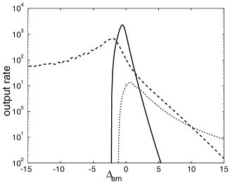
Figure 8: Population output rate from a finite temperature condensate with an RF coupler. Solid line, condensate component. Dashed line, stimulated quantum evaporation component. Dotted line, pair breaking component. Parameters: $T=0.5T_{c}$ $(150\hbar\omega/k)$, $\mu=2.3\hbar\omega/k$ , $N_{t}=2000$ atoms.

A key feature of the output coupling that is readily apparent in this figure is how the detuning $\Delta_{em}$ controls the character of the output field. For $\Delta_{em}<-\mu,$ only the thermal quasiparticles are ejected from the trap, as we expect from energy conservation (see Eq.(56)): only the quasiparticles have sufficient energy to absorb this amount of energy from the radiation field. For $\Delta_{em}>-\mu,$ up to $\Delta_{em}\approx\mu,$ fully coherent condensate dominates the output (see also Eq.(53)). Finally for $\Delta_{em}>\approx-\mu,$ both pair breaking (where the energy of the initial condensate atom plus the photon can be left in the trap) and thermal evaporation can occur.

As a final comment, we note that the processes of stimulated thermal evaporation and pair breaking reduce the coherence of the output field. Choi et al.[68] have calculated the coherence functions $g^{(1)}(x_{1},x_{2},t)$ and $g^{(2)}(x_{1},x_{1},t)$ and shown that even in the condensate dominated regime, the first order coherence is degraded, and $g^{(2)}$ exhibits symptoms of atom bunching.

8 Acknowledgements

RJB is grateful for many instructive conversations over the past few years with Professors C. Gardiner and K. Burnett, which have helped shape this article. This research was supported by the Marsden Fund of New Zealand under contract PVT902.

CMS acknowledges collaborations with J. Hope, G.Moy, and N. Robins. Our work is supported by the Australian Research Council.

References

- [1] H.M. Wiseman, Phys. Rev. A 56, 2068 (1997); 57, 674 (1998).
- [2] C.M. Savage, S. Marksteiner, P. Zoller, in “Fundamentals of quantum optics III”, ed. F. Ehlotzky (Springer 1993).
- [3] Ch.J. Bordé, Phys. Lett. A 204, 217 (1985); Ann. Phys. Fr. 20, 477 (1985); in Proc. of the 12th Int. Conference on Laser Spectroscopy, eds. M. Inguscio, M. Allegrini, A. Sasso (World Scientific 1995).
- [4] M. Olshanii, Y. Castin and J. Dalibard, Proc. of the 12th Int. Conference on Laser Spectroscopy, edited by M. Inguscio, M. Allegrini and A. Sasso (World Scientific 1995).
- [5] R.J.C. Spreeuw et al., Europhysics Letters 32, 469 (1995).
- [6] M. Holland et al., Phys Rev. A 54, R1757 (1996).
- [7] M.-O. Mewes, et al., Phys. Rev. Lett. 78, 582 (1997).
- [8] K. Helmerson, D, Hutchinson, K. Burnett, and W.D. Phillips, Physics World, p. 31, August (1999).
- [9] W. Ketterle, Physics Today 52 no. 12, 30 (1999).
- [10] A. Peters, Keng Yeow Chung, S. Chu, Nature 400, 849 (1999).
- [11] L. Deng et al., Nature 398, 218 (1999).
- [12] H.-A. Bachor, A guide to experiments in quantum optics (Wiley-VCH, 1998).
- [13] W. Ketterle and H.-J. Miesner, Phys. Rev. A 56, 3291 (1997).
- [14] B.P. Anderson and M.A. Kasevich, Science 282, 1686 (1998).
- [15] J.L. Martin, J. Phys. B 32, 3065 (1999).
- [16] I. Bloch et al., Phys. Rev. Lett. 82, 3008 (1999); Nature 403, 166 (2000).
- [17] E.W. Hagley, L. Deng, M. Kozuma, J. Wen, K. Helmerson, S.L. Rolston, W.D. Phillips, Science 283, 1706 (1999).
- [18] K. Molmer, Phys. Rev. A 55, 3195 (1997).
- [19] C.W. Gardiner and P. Zoller, Phys. Rev. A 58, 536 (1998).
- [20] E.M. Lifshitz and L.P. Pitaevskii, Statistical Physics, part 2, (Pergamon Press 1980).
- [21] M. Edwards and K. Burnett, Phys. Rev. A 51, 1382 (1995).
- [22] A.E. Siegman, Lasers (University Science Books, California 1986).
- [23] L. Mandel and E. Wolf, Optical Coherence and Quantum Optics (1995).
- [24] A.L. Schawlow and C.H. Townes, Phys. Rev. 112, 1940 (1958).
- [25] D.F. Walls and G.J. Milburn, Quantum Optics (Springer Verlag: Berlin 1994).
- [26] R.J. Glauber, Phys. Rev. 130, 2529 (1963).
- [27] M.R. Andrews et al., Science 275, 637 (1997).
- [28] K. Huang, Statistical Mechanics, (Wiley,1987).
- [29] M.O. Mewes et al., Phys. Rev. Lett. 77, 416 (1996).
- [30] M. Holland, et al., Phys. Rev. Lett. 78, 3801 (1997).
- [31] E.A. Burt, et al., Phys. Rev. Lett. 79, 337 (1997).
- [32] Yu. Kagan, B.V. Svistunov, G.V. Shlyapnikov, JETP Lett. 42, 209 (1985).
- [33] E.V. Goldstein and P. Meystre, Phys. Rev. Lett. 80 5036 (1998); E.V. Goldstein, O. Zobay, P. Meystre, Phys. Rev. A 58, 2373 (1998).
- [34] M. Naraschewski and R.J. Glauber, Phys. Rev. A 59, 4595 (1999).
- [35] G.M. Moy, J.J. Hope, C.M. Savage, Phys. Rev. A 59, 667 (1999).
- [36] G.M. Moy, J.J. Hope, C.M. Savage, Phys. Rev. A 55, 3631 (1997).
- [37] A.M. Guzman, M. Moore, P. Meystre, Phys Rev. A 53, 977 (1996).
- [38] H.M. Wiseman and M.J. Collett, Physics Lett. A 202,246 (1995).
- [39] H.M. Wiseman, A. Martins, D.F. Walls, Quant. Semiclass. Opt. 8 737 (1996).
- [40] R.J. Ballagh, K. Burnett, T.F. Scott, Phys. Rev. Lett. 78 1607 (1997).
- [41] W. Zhang and D.F. Walls, Phys. Rev. A 57 1248 (1998).
- [42] B. Kneer et al., Phys. Rev. A 58 4841 (1998).
- [43] N. Robins, C.M. Savage, E. Ostrovskaya, in Dan Walls Memorial Volume, eds. H. Carmichael, R. Glauber, M. Scully, in press (Springer, 2000).
- [44] H.M. Wiseman and M.J. Collett, Phys. Lett. A 202 246 (1995).
- [45] J.J. Hope, Phys. Rev. A 55 R2531 (1997).
- [46] G.M Moy and C.M. Savage, Phys. Rev. A 56 1087 (1997).
- [47] J.J. Hope, G.M Moy, M.J. Collett, C.M. Savage, Phys. Rev. A 61 023603 (2000).
- [48] D.W. Snoke and J.P. Wolfe, Phys. Rev. B 39, 4030 (1989); D. Semikoz and I.I. Tkachev, Phys. Rev. Lett. 74, 3093 (1995).
- [49] H.T.C. Stoof, Phys. Rev. Lett. 66, 3148 (1991); Phys. Rev. A 49, 3824 (1994); Phys. Rev. Lett. 78, 768 (1997).
- [50] Yu. Kagan, B.V. Svisunov, G.V. Shlyapnikov, Sov. Phys. JETP 75, 387 (1992); Yu. Kagan and B.V. Svisunov Phys. Rev. Lett. 79, 3331 (1997).
- [51] C.W. Gardiner and P. Zoller, Phys. Rev. A 55, 2902 (1997).
- [52] C.W. Gardiner, P. Zoller, R.J. Ballagh, M.J. Davis, Phys. Rev. Lett. 79, 1793 (1997).
- [53] C.W. Gardiner and P. Zoller, Phys. Rev. A 58, 536 (1998).
- [54] C.W. Gardiner, M.D. Lee, R.J Ballagh, M.J. Davis and P. Zoller, Phys. Rev. Lett. 81, 5266 (1998).
- [55] C.W. Gardiner and P. Zoller, Phys. Rev. A 61, 033601 (2000).
- [56] M. D. Lee and C. W. Gardiner, cond-mat/9912420, Phys. Rev. A in press.
- [57] H.-J. Miesner, D.M. Stamper-Kurn, M.R. Andrews, D.S. Durfee, S. Inouye, W. Ketterle, Science 279, 1005 (1998).
- [58] C.W. Gardiner, Phys. Rev. A 56, 1414 (1997).
- [59] M. J. Davis, C. W. Gardiner, R. J. Ballagh, cond-mat/9912439 , Phys. Rev. A in press.
- [60] M. Holland, J. Williams, J. Cooper, Phys. Rev. A 55, 3670 (1997).
- [61] M. Bijlsma, E. Zaremba, H. T. C. Stoof, cond-mat/0001323 .
- [62] M.-O. Mewes, M. R. Andrews, D. M. Kurn, D. S. Durfee, C. G. Townsend, W. Ketterle, Phys. Rev. Lett. 78, 582 (1997).
- [63] I. Bloch, T. W. Hänsch and T. Esslinger, Phys. Rev. Lett. 82, 3008 (1999).
- [64] H. Steck, M. Naraschewski, H. Wallis, Phys. Rev. Lett. 80, 1 (1998).
- [65] B. Jackson, J. F. McCann, C. S. Adams, J. Phys. B 31, 4489 (1998).
- [66] M. Edwards, D. A. Griggs, P. L. Holman, C. W. Clark, S. L. Rolston, W. D. Phillips, J. Phys. B 32, 2935 (1999).
- [67] Y. Japha, S. Choi, K. Burnett, Y. Band, Phys. Rev. Lett. 82, 1079 (1999)
- [68] S. Choi, Y. Japha, K. Burnett, Phys. Rev. A 61, 063606 (2000).