Power, Levy, Exponential and Gaussian Regimes in Autocatalytic Financial Systems

Abstract

We study by theoretical analysis and by direct numerical simulation the dynamics of a wide class of asynchronous stochastic systems composed of many autocatalytic degrees of freedom. We describe the generic emergence of truncated power laws in the size distribution of their individual elements. The exponents $\alpha$ of these power laws are time independent and depend only on the way the elements with very small values are treated. These truncated power laws determine the collective time evolution of the system. In particular the global stochastic fluctuations of the system differ from the normal Gaussian noise according to the time and size scales at which these fluctuations are considered. We describe the ranges in which these fluctuations are parameterized respectively by: the Levy regime $\alpha<2$, the power law decay with large exponent ($\alpha>2$), and the exponential decay. Finally we relate these results to the large exponent power laws found in the actual behavior of the stock markets and to the exponential cut-off detected in certain recent measurement.

1 Introduction

It was realized since a very long time that the fluctuations $r(t)$ of stochastic systems made of many degrees of freedom are not generically distributed by Gaussian probability distributions Mandelbrot63 ; Stanley95 . On the theoretical side, P. Levy Levy37 discovered at the beginning of this century that the central limit theorem allows for a family of distributions which decay at infinity as a power law:

$$P(r)\sim r^{-1-\alpha}\ \ {\rm with}\ \ 0<\alpha<2$$ (1)

These distributions can be thought as the limit distributions for random walks with steps of sizes $s_{i}$ distributed by a power law

$$P(s)\sim s^{-1-\alpha}.$$

Such processes were named Levy flights Schlesinger95 .

In nature, the situation turns out to be more complicated: many of the measurements produced probability distribution functions which look like Levy distributions for a certain range of the stochastic variable but are cut off. That is, they change their character above a certain threshold, e.g., by becoming exponentials or changing to a power decay with $\alpha>2$ as found for the returns of stock market data Stanley95 ; Lux96 ; Gopikrishnan99 ; Huang00 . Particular examples of such distributions were studied under the name of truncated Levy flight Mantegna94 . As required by the central limit theorem, for very large time intervals $t$, these distributions cross-over into a quite Gaussian behavior.

Recently, both the power law probability distribution of the individual steps and the truncated Levy distribution of the fluctuations were explained generically by a series of Generalized Lotka-Volterra (GLV) models Solomon96 ; Solomon98 ; Biham98 ; Malcai99 . These models represent realistic financial, biological and social systems composed of many autocatalytic and competing stochastic subsystems Solomon98 .

In this paper we study the exact nature of the cut-off region and the details of the cross-over process in the framework of the GLV models. We especially describe the emergence of the tail distribution with $\alpha\approx 3$ power law and the exponential cut-off. The theoretical analysis below yields well defined quantitative predictions on the various temporal and geometric properties of the probability distribution functions, which are verified by the numerical simulations and compared with the actual measurements of the Hong Kong stock market. Most of the results extend however to other models too.

2 Theoretical analysis

2.1 Autocatalytic systems and power law

The analysis here applies to a large range of dynamical models Solomon98 . For definiteness we consider a specific system $W(t)$ formed of subsystems $w_{i}(t)$, $i=1,2,...,N$:

$$W(t)=w_{1}(t)+w_{2}(t)+...+w_{N}(t)$$ (2)

distributed by a power law cumulative distribution function:

$$P(>w)=[w/w_{min}(t)]^{-\alpha}$$ (3)

with the corresponding density $P(w)\propto w^{-1-\alpha}$, where $w_{min}$ is some lower cut-off

$$w_{min}(t)=q\bar{w}(t),$$ (4)

i.e., usually given in terms of a fraction $q$ of the average $\bar{w}(t)=W(t)/N$.

Such distributions emerge naturally in autocatalytic systems Solomon96 ; Solomon98 ; Biham98 ; Malcai99 of the generic form:

$$w_{i}(t+1)=\lambda(t)w_{i}(t)+a{\bar{w}}(t)-bw_{i}(t){\bar{w}}(t).$$ (5)

For the purpose of this paper we describe them by a simple dynamics Solomon96 ; Malcai99 which consists in choosing randomly at each time step for updating one of the $w_{i}$’s and multiplying it by a random factor $\lambda(t)$ extracted at each time from a probability distribution $\rho(\lambda)$:

$$w_{i}(t+1)=\lambda(t)w_{i}(t),$$ (6)

with the lower cut-off

$$w_{i}(t+1)\geq q\bar{w}(t).$$ (7)

That is, the updated variable $w_{i}(t+1)$ is constrained to be not smaller than a lower bound $q\bar{w}(t)$, i.e.,

$$w_{i}(t+1)={\rm max}\{w_{i}(t+1),q\bar{w}(t)\},$$

where $\bar{w}(t)$ is the average value calculated at earlier time $t$. Note that all the $w_{i}$’s are strictly positive and therefore

$$w_{i}(t)<W(t)=N\bar{w}(t).$$ (8)

In systems of the type Eqs. (6) and (7), it has been shown Solomon96 ; Malcai99 that even if the system is not stationary the power law Eq. (3) holds, and for given $N$ and $q$ in the range $1>q\gg 1/\ln N$, the exponent $\alpha$ is given by the relation:

$$\alpha=1/(1-q)$$ (9)

Usually in financial applications $q\sim 1/3$, and then the exponent $\alpha\sim 1.5$ within the stable Levy regime.

During our analysis of this section we will take the distribution $\rho(\lambda)$ centered around 1:

$$\lambda(t)=1+g(t),$$ (10)

and consisting of just 2 equally probable values

$$g(t)=\pm M.$$ (11)

The conclusions of our analysis are not changed if one assumes an arbitrary distribution $\rho(\lambda)$ with finite strictly positive support.

Here we are interested in the distribution of the ”returns” :

$$r(\tau)=[W(t+\tau)-W(t)]/W(t)$$ (12)

as a function of the time interval $\tau$. The use of the term ”return” in (12) as a measure of the fluctuation in the system is borrowed from the financial applications where $W(t)$ is the stock market index and $r(\tau)$ is the relative gain/loss one incurs after a time lapse $\tau$.

Since the variation of $W(t)$ at each time coincides with the variation of the individual $w_{i}(t)$ which happened to be randomly selected for updating by Eq. (6) at time $t$, the value of $r(\tau)$ as defined in Eq. (12) is the result of a random walk

$$r(\tau)=\sum\limits_{k}s_{i}(t+k),$$ (13)

with steps $s_{i}(t+k)$, $k=0,1,...,\tau-1$ of sizes comment1 :

$$s_{i}(t+k)=[w_{i}(t+k+1)-w_{i}(t+k)]/W(t),$$ (14)

which according to Eqs. (6), (10) and (11) is written as:

$$s_{i}(t+k)=\pm Mw_{i}(t+k)/W(t).$$ (15)

Therefore, the sizes of the (absolute values of the) individual steps $s_{i}(t+k)$ in the random walk/flight process $r(\tau)$ (Eq. (13)) have a probability distribution function similar to Eq. (3) (up to the factor $M/W$):

$$S(>s)=[s/s_{min}]^{-\alpha},$$ (16)

where $s_{min}=Mw_{min}/W=Mq/N$.

2.2 Origin of truncation in autocatalytic systems

A crucial fact of the present paper is that the power law distribution Eq. (16) from which the individual steps Eq. (14) composing the random walk $r(\tau)$ through Eq. (13) are selected is truncated from above note2 .

Indeed, since $w_{i}<W$ for any $i$ as shown in Eq. (8), the individual steps Eq. (14) cannot be larger than the fixed value $M$, i.e.

$$S(>M)=0.$$ (17)

Note that this bound in the size of the individual steps of the random walk $r(\tau)$ does not depend on the number $N$ of participants in the game nor on the exponent $\alpha$ of the power law, nor on the lower cut-off $w_{min}$. One cannot therefore hope that the effects of this upper bound would somewhat become irrelevant, and as seen below (Eq. (26)), by increasing $N$ one can only delay the time

$$\tau_{max}=N^{\alpha}$$

by which these effects become dominant. Therefore, for finite time intervals $\tau$ and infinite $N$, the effect of the truncation disappears (together with the vanishing of the amplitude of elementary fluctuations $|r(1)|<N^{1-\alpha}$ Solomon98 ). In finance, however, we are generically in the opposite limit, e.g. a finite number of traders trading for very long time intervals $\tau$ which allow them to perform a total number of elementary trading operations much larger than $\tau_{max}$.

Our goal in the sequel will be therefore to follow in detail the process by which the $\tau=1$ (truncated at $r>M$) power distribution

$$R(>r,1)=S(>r)=[r/s_{min}]^{-\alpha}=[r/(qM/N)]^{-\alpha}$$ (18)

evolves for increasing time interval $\tau$, and then approaches the infinite time ($\tau\gg\tau_{max}$) Gaussian distribution. We will analyze explicitly $R(>r,\tau)$ only for positive $r$’s to avoid unnecessary complication. However, the analysis for negative $r$ values is very similar.

In fact, for the probability distribution function of returns $R(>r,\tau)$ one obtains a symmetric probability density $R(r,\tau)={dR(>r,\tau)}/{dr}$ which for $\tau=1$ coincides with the $S(s)={dS(>s)}/{ds}$ probability density. On a log-log scale the probability density $\ln R(r,1)$ vs. $\ln r$ is a line ending sharply around $r=s_{min}$. We will see that for larger $\tau$ values the sharp tip will erode into a flatter ”dome” and the complete/exact vanishing of the distribution at the upper cut-off $r=M$ will evolve into a steep but continuous decay.

2.3 Power law and truncation for $\tau<\tau_{max}$

The probability $R(>r,\tau)$ to reach after a $\tau$-steps walk a distance $r$ or larger is of course a result of the probabilities of the $\tau$ individual steps which compose the ”walking”/”traveling”/”flying” Mantegna94 process. Therefore its characteristics depend on the 3 crucial properties of the individual steps distribution $S(>s)$ obtained from Eqs. (16)–(18):

1. The great majority of the individual steps $s_{i}$ are of order $s_{mean}$ (the average of $s_{i}$) and less, i.e., in the range:

   $$s_{min}=qs_{mean}=qM/N<s<2s_{mean}=2M/N.$$ (19)

2. The steps of larger sizes (say larger than $2s_{mean}$) are very rare:

   $$R(>2M/N,1)\sim(q/2)^{\alpha}<0.07$$ (20)

   (We take $\alpha\sim 1.5$ as in real wealth distribution Levy97 ).

3. There are no individual steps in $r(\tau)$ of size larger than $M$:

   $$R(>M,1)=0.$$ (21)

Due to those properties, as one increases the time interval $\tau$ from $1$, the initial (truncated) power law distribution Eq. (18) $R(>r,1)=S(>r)$ is not significantly affected for most of the $r$ range. For small $\tau$’s, the corrections to the power law are in fact limited only to the lower and upper cut-off regions and are analyzed below.

2.3.1 The low $r$ ”dome”-like region

The low $r$ region in $R(>r,\tau)$ is affected even for small $\tau>1$ because there is a large probability that all of the $\tau$ steps are of the order $s_{mean}$ and lower. Consequently, the probability $R(>r,\tau)$ for values $r<\tau s_{mean}=\tau M/N$ is not given anymore by the probability $R(>r,1)=S(>r)$ of obtaining it through a single step, but rather by a combinatoric sum of probabilities of having $\tau$ (small, positive and negative) steps summing up to $r$. This is of course very similar to the way one estimates (through Poisson/Binomial expansion) the probability of a distance $r$ after a $\tau$ steps Gaussian walk. The consequence is a smoothening of the sharp end at $R(r=0,\tau)$. This concretizes in the appearance of a ”dome”-like shape in the central region (around $r=0$) of the $R(r,\tau)$ probability density.

To estimate (the time dependence of) the extent of the ”dome”-like region, we demand that the probability of achieving distances $r$ through $2$ or more steps is larger than the probability of achieving it through one step. Since $(\tau S(r/2))^{2}$ is the probability of having during $\tau$ steps at least $2$ steps of sizes at least $r/2$, and $\tau S(r)$ is the probability of having at least one of the $\tau$ steps of size at least $r$, the condition describing the ”dome”-like region is:

$$(\tau S(r/2))^{2}>\tau S(r),$$

which by substituting the power law Eq. (16) for $S(>s)$ becomes:

$$\{\tau[r/(2s_{min})]^{-\alpha}\}^{2}>\tau(r/s_{min})^{-\alpha},$$

gives the central dome region:

$$r<4s_{min}\tau^{1/\alpha}=4qM/N\tau^{1/\alpha}.$$ (22)

since $q$ is in (finance markets) practice not far from $1/4$ we denote

$$r_{dome}=s_{mean}\tau^{1/\alpha}=M/N\tau^{1/\alpha}$$ (23)

and with this notation, the condition Eq. (22) becomes

$$r<r_{dome}.$$ (24)

Thus, the power law Eq. (18) remains unchanged in the range

$$r_{dome}<r<M,$$ (25)

and the power law region disappears completely when the upper and lower limits of this interval coincide:

$$r_{dome}=M,$$

i.e. (cf Eq. (23) by the time that

$$\tau^{1/\alpha}M/N=M$$

holds. This gives the maximal time for which one still has a power-like region:

$$\tau_{max}=N^{\alpha}.$$ (26)

Since the power law region is the crucial feature of the (truncated) Levy distribution, $\tau_{max}$ is essentially the maximal time interval for which the returns (12) still maintain a Levy-like probability distribution. Note that this value for $\tau_{max}$ agrees with the early estimations of Ref. Mantegna94 based on the scaling $R(0,\tau)\sim\tau^{1/\alpha}$ of the probability distribution peak.

2.3.2 The extremely large $r>M$ region

In the upper cut-off region $r>M$ the probability distribution function $R(>r,\tau)$ is affected by increasing $\tau$ from $1$ to larger values. Indeed, while values $r>M$ are completely disallowed for $\tau=1$ because of the truncation Eq. (21), for $\tau>1$ one can have $r$’s in the range $M<r<\tau M$. The probability of obtaining such values of $r$ corresponds to the probability of selecting repeatedly for updating (by Eq. (6)) the largest $w_{i}$’s. For instance, the probability of obtaining a value $r>KM$ (with $K$ a small integer) is roughly the probability of extracting out of the $\tau$ steps at least $2K$ times steps of size at least $M/2$. For $K<<\tau$ this is basically the probability of at least one step of size at least $M/2$ multiplied by $\tau$ and risen at the power $2K$:

$$R(>r=KM,\tau) \sim [\tau S(>M/2)]^{2K}$$

$$\sim [\tau(M/(2s_{min}))^{-\alpha}]^{2K},$$

which can also be written as

$$R(>r,\tau)\sim\left[\left({N\over{(2q)^{\alpha}\tau}}\right)^{2}\right]^{-r/M},$$ (27)

i.e., $R(>r,\tau)$ decays exponentially with $r$. Values larger than $KM$ are still rigorously disallowed.

To sum up the results for small and moderate intervals $\tau<\tau_{max}$: except for the central dome region $|r|<r_{dome}$ and the extremely large $|r|>M$ region, the probability distribution function $R(>r,\tau)$ is similar to the single step probability $R(>r,1)=S(>r)$ (Eq. (18)). This is intuitively explained by the fact that the probability to arrive after $\tau$ random steps at large (but less than $M$) $r$ values is dominated by the probability of having a single step of order $r$.

The 3 regions above: central dome region $r<r_{dome}$, the Levy-like power law region, and the extremely large $r>M$ exponential region are the main features of the distribution $R(>r,\tau)$ for intervals $\tau<\tau_{max}$.

2.4 Cross-over for $\tau>\tau_{max}$

The time evolution of the $R(>r,\tau)$ shape depends on the fact that while the upper cut-off region (beyond which the power law fails) $r>M$ is fixed, the ”dome” region expands with $\tau$ according to Eq. (23). (Intuitively this is because, as one increases the number of time steps $\tau$, one can reach larger values of their sum $r(\tau)$ even if each of the individual steps is of order $\bar{w}$ or less). As seen above, this leads for intervals $\tau>\tau_{max}$ (Eq. (26)) to the disappearance of the intermediate Levy-like power law region in the $R(>r,\tau)$ distribution. After this time, the central dome will keep expanding on the expense of the $r>M$ cut-off region.

As it expands, the dome will assume a shape closer and closer to a Gaussian. This will be consistent with the central limit theorem as the involved elementary steps will be ultimately distributed on a finite support $s_{min}<s<M$ of quite limited extent compared with the $r\gg M$ range of values probed by the dome for very large times.

Indeed, for time intervals $\tau\gg\tau_{max}$, the probability of many steps of size close to $M$ is not negligible. Thus the dynamics consists in a random walk of individual steps of size distributed within the finite support between $0$ and $M$. The distribution becomes a Gaussian whose expansion is dominated by the largest steps $M$. Since there will be roughly one step of size $M$ per $\tau_{max}=N^{\alpha}$ interval, the Gaussian width will expand as

$$\sigma(\tau)=M(\tau/\tau_{max})^{1/2}=MN^{-\alpha/2}\tau^{1/2}.$$ (28)

For returns much larger than this, i.e., $r>\sigma(\tau)$, the exponential regime Eq. (27) will still survive.

The above results can be verified by the numerical simulations shown below. Moreover, for time interval $\tau>\tau_{max}$ but not too large, the power law distribution of returns with exponent well outside the stable Levy regime of $\alpha<2$ can be obtained in the simulations, with the exponential cut-off effect.

Figure 1: Semi-plot of the probability density of returns $r(\tau)$ (defined by Eq. (29)) for different time intervals $\tau=1$, $500$, and $12000$ ($N=500$).

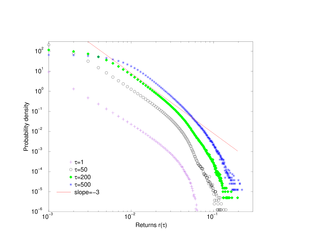
Figure 2: The probability density of the positive returns $r(\tau)$ (defined by Eq. (29)) in log-log plot for time intervals $\tau=1$, $50$, $200$, and $500$ ($N=500$, calculated after $t=10^{5}N$ updatings), with a straight line of slope $-3$ ($\alpha=2$) for comparison.

3 Numerical simulations

We have performed the computer simulations of autocatalytic system described by Eqs. (6) and (7), where the random factor $\lambda$ is set to uniformly distribute in the range $0.9<\lambda<1.1$. In our simulations the number of subsystems $N=500$, and the lower bound factor $q=0.3$. Thus, according to relation (9), the exponent $\alpha$ of the power law distribution of $w$ is about $1.4$, which has been verified by previous simulations Malcai99 .

Here we numerically study the distribution of the fluctuations or ”returns”

$$r(\tau)=\ln W(t+\tau)-\ln W(t)$$ (29)

for different time intervals $\tau$, to compare with the above analytic results. Note that in Eq. (29) we use the logarithmic difference for the definition of return, as in usual financial applications, which is approximately the relative change Eq. (12) if the change is small. Note that due to the lower bound $q\bar{w}$ (Eq. (7)), in this system $W(t)$ has an increasing trend, which makes the return (29) more possible to be positive, especially for large $\tau$. Thus, in our simulation results shown below, a maximum at positive finite $r$ is obtained for large $\tau$ distribution. In general, one could normalize $W(t)$ ($w_{i}(t)$) by a value $\exp(\kappa t/N)$ with $\kappa$ constant, for detrending, and then Eq. (29) would change by a constant: $r(\tau)\rightarrow r(\tau)-\kappa\tau/N$, which does not influence the statistical properties.

With $N=500$ and $\alpha\sim 1.4$, we have $\tau_{max}=N^{\alpha}\sim 6000$ from Eq. (26), and the behaviors obtained for small and large $\tau$ are different, as shown in Fig. 1 for $\tau=1$, $500$, and $12000$. With the increase of time interval $\tau$, the sharp peak of the distribution curve is smeared out into a dome-like shape, similar to the empirical findings of financial markets Gopikrishnan99 .

3.1 $\tau<\tau_{max}$

The numerical results of probability density $R(r,\tau)$ for time intervals $\tau=1$ (pluses), $50$ (circles), $200$ (diamonds) and $500$ (stars) are presented in Fig. 2. The measurement was performed after $t=10^{5}N$ updatings, and averaged over $100$ runs for $\tau=1$ and $800$ runs for $\tau\geq 50$. The results for $\tau=1$ are just what we derive in Sec. 2.2, i.e., a straight line in log-log plot with sharp end, obeying Eq. (18) with $\alpha$ about $1.5$, and a cut-off for large $r$.

For intervals larger than $1$, the 3 regions obtained analytically in Sec. 2.3 are clearly shown in the log-log plots of Fig. 2. The first one is the central ”dome”-like region for small $r$, with larger extent for larger $\tau$, as predicted in Eq. (23). For small interval $\tau=50$, the derivative at small $r$ is not close to zero, that is, the sharp end persists, while it flattens into the dome for larger intervals of $200$ and $500$. In the intermediate $r$ range, the power law behavior similar to Eq. (18) is presented. For small values of $\tau$ ($\leq 200$ in Fig. 2), the exponent $\alpha$ is within the stable Levy regime, that is, $0<\alpha<2$, however, for larger $\tau$ (say $500$) one can obtain the exponent $\alpha>2$, which is similar to the phenomenon shown below for $\tau>\tau_{max}$.

When the return $r$ is large, the deviation from the straight line and the curvature in log-log plot can be observed (see Fig. 2), which is just the cut-off effect described above, that is, the exponential decay for far tail distribution (similar to Eq. (27)).

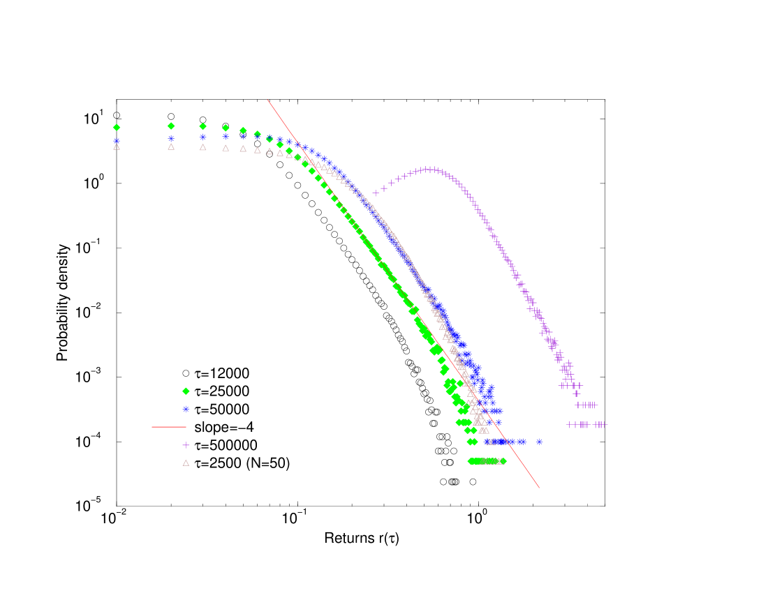
Figure 3: The probability density of the positive returns $r(\tau)$ in log-log plot for large time intervals $\tau=12000$, $25000$, $50000$, and $500000$ of $N=500$, as well as $\tau=2500$ of $N=50$ (calculated after $t=10^{5}N$ updatings), with a straight line of slope $-4$ ($\alpha=3$) which fits the data for a few orders of magnitude. For $\tau=500000$, only part of the distribution is shown.

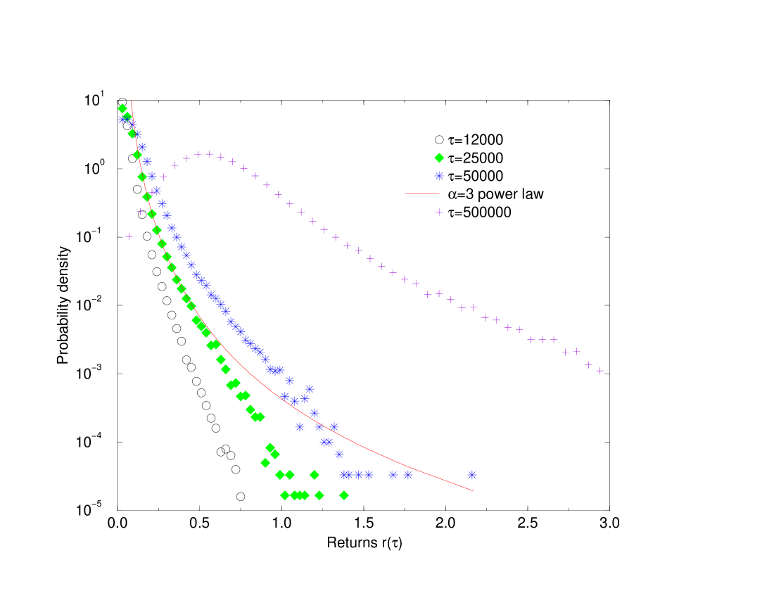
Figure 4: Replot of Fig. 3 on a semi-log scale, using larger bin size.

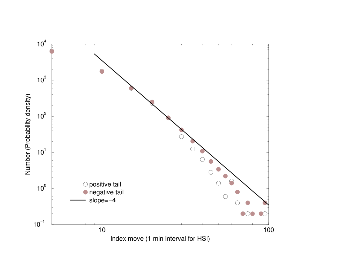
Figure 5: Log-log plot of the probability density of 1 minute index moves for the Hong Kong HSI (from Jan. 1994 to Dec. 1997), with the skip of the first 20 minutes in daily opening Huang00 . A straight line with slope $-4$ is also shown.

3.2 $\tau>\tau_{max}$

The crucial results of this paper are for large time interval $\tau$, which corresponds to realistic time scale observed in nature (e.g., financial markets). These results are the consequences of the truncation in this autocatalytic system, as discussed analytically above, and can be compared with those of the real market data.

We have calculated the return distribution for large $\tau$: $12000$, $25000$, and $50000$ (averaged over $1000$ runs), as shown in Fig. 3. Besides the dome-like shape for small $r$, what interests us is the power law region for intermediate and large returns. In this region the exponent $\alpha$ is about $3$, well beyond the stable Levy regime, but in agreement with the recent observations in real stock market Lux96 ; Gopikrishnan99 .

However, for extremely large returns, i.e., the far tail of the distribution, the exponential cut-off effect still remains, as shown in the bent of the log-log plots in Fig. 3. To see more clearly, we replot Fig. 3 on a semi-log scale to Fig. 4, where the tail of return distribution looks like a straight line, indicating an exponential-type behavior. This exponentially asymptotic decay was not detected in the empirical findings of Lux96 and Gopikrishnan99 , but agrees with the most recent observation in Hong Kong stock market Huang00 as shown in Sec. 4 below.

To see whether this phenomenon of $\alpha=3$ power law and exponential cut-off is related to finite size effect or is intrinsic, we perform the simulations for $N=50$, and present the result of $\tau=2500$ in Fig. 3. The range of power law behavior ($\alpha\sim 4.5$ for $N=50$) may be slightly shorter than that of the larger system $N=500$. Thus, the power law region before the exponential cut-off is expected to extend for large system size ($N$), which has been verified by simulations for $N=5000$.

For very large $\tau$, i.e., $\tau\gg\tau_{max}$, the distribution of returns is to approach Gaussian based on the central limit theorem (also expected in Sec. 2.4), which has been found in reality Gopikrishnan99 . In Fig. 3 the result for $\tau=500000$ is also shown with the Gaussian-like behavior for not too large $r$ value, which exhibits as a parabola in semi-log plot (Fig. 4) note3 . The exponential-type decay is still found in Fig. 4 for extremely large $r$ as expected.

4 Discussion and conclusion

In finance, the tradings of the various investors $w_{i}$ are performed independently. Therefore, the natural time measure is not the number of operations but the number of operations divided by the number of components $N$:

$$T=\tau/N.$$ (30)

Thus, for the power law behavior of large $\tau$ ($500$, $12000$, $25000$, and $50000$) shown in Figs. 2 and 3 with exponent well outside the Levy regime, the corresponding $T$ values are $1$, $24$, $50$, and $100$ (for $N=500$ in our simulations). Although in real market the time interval between transactions of stocks is irregular, one could estimate from the market transaction data Plerou99 that the unit scale $T=1$ here approximately corresponds to several minutes of real time.

It is interesting to compare the results of this autocatalytic system with actual measurements of the stock markets. The power law behavior with exponent $\alpha$ about $3$ was observed in recent empirical studies on S&P 500 Gopikrishnan99 and German DAX Lux96 , consistent with the results shown in Fig. 3 for intermediate and large returns, but not the exponential cut-off. However, very recently it has been found from the Hang Seng Index (HSI) of Hong Kong Huang00 that the index fluctuations for the first few minutes of daily opening behave very differently from those of the other times, due to much higher influences of exogenous factors at the opening. As shown in Fig. 5, if we skip the data in the first $20$ minutes of each trading day, the distribution for 1 minute time interval index move (defined as ${\rm index}(t+\tau)-{\rm index}(t)$, with the statistical properties very similar to that of Eq. (29) for the high-frequency regime, e.g., interval $\tau=1$ min) exhibits the phenomenon of exponential-type decay Tang00 after the transient $\alpha=3$ power law region, in agreement with our simulation results of Figs. 4 and 2 ($\tau=500$). Moreover, real markets show the tendency of a crossover towards a Gaussian for long enough times Gopikrishnan99 , which has also been found in our system (see Figs. 3 and 4 for very large interval $\tau=500000$ and intermediate $r$).

In order to account for the experimentally observed volatility correlations, one may follow Ref. Solomon98 and feed back the absolute market returns (Eq. (29)) into the individual gain factor (6). A possible form is using:

$$\lambda(t)=\exp[\langle r\rangle+\eta(\langle r^{2}\rangle-\langle r\rangle^{2})^{1/2}]$$

where the angle brakets indicate averages over the last $\tau$ steps and $\eta$ is a Gaussian random number of zero mean and unit variance. The numerical results for these more realistic simulations will be presented elsewhere.

In summary, we have shown that the simple random multiplicative model of Ref. Solomon96 , with a lower cut-off, gives many of the properties found in reality and in more complicated models, like e.g. the percolation model Cont00 : power law with effective exponent $\alpha$ near 3, rounding of the singularity at zero returns, crossover to Gaussian for long times. We still have to work on implementing volatility clustering, multifractality, lack of up-down and time reversal symmetry, and correlation between traded volume and volatility. Only the original random walk model of Bachelier seems to us simpler than the present model but of the above properties it has only a Gaussian distribution.

- (1) B.B. Mandelbrot, J. Business 36, 394 (1963).
- (2) R.N. Mantegna, H.E. Stanley, Nature 376, 46 (1995).
- (3) P. Lévy, Theorie de l’Addition des Variables Aleatoires (Gauthier-Villiers, Paris, 1937).
- (4) M.F. Shlesinger, U. Frisch, G. Zaslavsky (eds), Lévy Fights and Related Phenomena in Physics (Springer, Berlin, 1995).
- (5) T. Lux, Appl. Financial Economics 6, 463 (1996).
- (6) P. Gopikrishnan, V. Plerou, L.A.N. Amaral, M. Meyer, and H.E. Stanley, Phys. Rev. E 60, 5305 (1999).
- (7) Z.F. Huang, e-print, cond-mat/0006145 (to appear in Physica A).
- (8) R.N. Mantegna, H.E. Stanley, Phys. Rev. Lett. 73, 2946 (1994).
- (9) M. Levy, S. Solomon, Int. J. Mod. Phys. C 7, 595 (1996); S. Solomon, M. Levy, ibid. 7, 745 (1996).
- (10) S. Solomon, in Decision Technologies for Computational Finance, edited by A.-P. Refenes, A.N. Burgess, J.E. Moody (Kluwer Academic Publishers, 1998), pp. 73-86.
- (11) O. Biham, O. Malcai, M. Levy, S. Solomon, Phys. Rev. E 58, 1352 (1998).
- (12) O. Malcai, O. Biham, S. Solomon, Phys. Rev. E 60, 1299 (1999).
- (13) In order not to complicate the notation we will not write in Eq. (13), but one should keep in mind that the selected for updating changes after each time step.
- (14) Moreover, the global condition introduces correlations between the step sizes of the Levy process. These correlations are not taken into account in the following theoretical analysis and might account for some of its differences with respect to the numerical (and experimental) results. We thank D. Stauffer for suggesting this to us.
- (15) M. Levy, S. Solomon, Physica A 242, 90 (1997).
- (16) The phenomenon that the parabola is shifted to the right is related to the fact that we used a large value for the volatility to reach faster the convergence of the numerical runs. In real financial systems this shift is unobservable for intraday fluctuations.
- (17) V. Plerou, P. Gopikrishnan, L.A.N. Amaral, X. Gabaix, H.E. Stanley, e-print, cond-mat/9912051.
- (18) L.H. Tang, Z.F. Huang, e-print, cond-mat/0007267.
- (19) R. Cont and J.P. Bouchaud, e-print cond-mat/9712318 = Macroeconomic Dynamics 4, 170 (2000).