Bose-Einstein condensation in shallow traps

Abstract

In this paper we study the properties of Bose-Einstein condensates in shallow traps. We discuss the case of a Gaussian potential, but many of our results apply also to the traps having a small quadratic anharmonicity. We show the errors introduced when a Gaussian potential is approximated with a parabolic potential, these errors can be quite large for realistic optical trap parameter values. We study the behavior of the condensate fraction as a function of trap depth and temperature and calculate the chemical potential of the condensate in a Gaussian trap. Finally we calculate the frequencies of the collective excitations in shallow spherically symmetric and 1D traps.

I Introduction

An atomic Bose-Einstein condensate [1, 2, 3] is an excellent tool for studying quantum many body phenomena, such as collective excitations. The particle interactions in these condensates are weak and thus even quantitave agreement between theory and experiments can be found. Recently a sodium condensate was trapped in an optical dipole trap [4]. Usually the potential of such trap is approximated by the parabolic potential, but the shallow nature of the optical dipole trap makes it clear that for suitably large condensates, the anharmonicity of the potential has to be taken into account.

In this paper we study how the shallowness of the potential changes the condensate properties. To enable an analytical approach we assume a Gaussian potential [5], but we expect that the qualitative features are valid also for other types of shallow traps. Bose-Einstein condensation in power-law potentials has been studied previously [6], but usually the potential has been assumed to be parabolic or absent. In Sec. II we calculate how the condensate fraction behaves as a function of temperature and how the parabolic approximation may underestimate the BEC transition temperature considerably. In Sec. III we calculate the chemical potential and estimate how many condensate particles can be trapped. Frequencies of the collective excitations are calculated in Sec. IV, and some concluding remarks are given in Sec. V.

II Condensate fraction

Particle interactions have a dramatic effect for particle density distribution, chemical potential and collective excitations of the condensate, but the transition temperature and the condensate fraction can be accurately calculated with the ideal gas model [7]. If there is a repulsive interaction between the trapped atoms, and the chemical potential is almost the same as the trap depth, we expect changes to the ideal gas results, but for now, the simple ideal gas model will suffice. In a harmonic trap the transition temperature $T_{c}$ is given by

$$k_{B}T_{c}=\hbar\left(\frac{N\omega_{x}\omega_{y}\omega_{z}}{\zeta(3)}\right)^{1/3},$$ (1)

where $\omega_{\alpha}$ is the trap frequency in direction $\alpha$ and $N$ is the particle number. The condensate fraction is then given by [8]

$$\frac{N_{c}}{N}=1-\left(\frac{T}{T_{c}}\right)^{3}.$$ (2)

In a Gaussian potential

$$V(x,y,x)=V_{1}\left[1-\exp\left(-\frac{x^{2}}{2\sigma_{x}^{2}}-\frac{y^{2}}{2\sigma_{y}^{2}}-\frac{z^{2}}{2\sigma_{z}^{2}}\right)\right]$$ (3)

condensate fraction can behave in a qualitatively different way. Using a phase space density [9]

$$f({\bf r},{\bf p})=\frac{1}{\exp(\beta H)-1},$$ (4)

where $H$ is the total energy, we can calculate the number of thermal particles as

$$N_{T}=\frac{1}{(2\pi\hbar)^{3}}\int\int d{\bf p}d{\bf r}f(\bf{r},\bf{p}).$$ (5)

Our trap has a finite depth and therefore we must introduce an appropriate $r$ dependent cut-off for the kinetic energies. After a short calculation we see that the number of thermal atoms is given by

$$N_{T} = \frac{16}{\pi}\left(\frac{mV_{1}}{\hbar^{2}}\right)^{3/2}\sigma_{x}\sigma_{y}\sigma_{z}$$ (7)

$$\int_{0}^{\infty}dx\int_{0}^{s_{max}}ds\frac{x^{2}s^{2}}{\exp(\beta V_{1}(s^{2}+1-\exp(-x^{2})))-1},$$

where $s_{max}=\exp(-x^{2})$.

When the trap has only a few eigenstates, the continuum approach fails and we should model the system using a discrete spectrum. If the potential is spherically symmetric and is approximated as a parabola, then the number of different energy levels is roughly $V_{1}/\hbar\omega=\sqrt{V_{1}m\sigma^{2}/\hbar^{2}}$. This provides a lower limit to the number of energy levels, since for a Gaussian trap the separation between adjacent levels becomes smaller as the energy increases (approaching zero as the energy approaches the trap depth). If the trap depth is very small, $V_{1}\approx 9\,\rm{nK}$ and $\sigma=15\,\rm{\mu m}$ the trap has roughly ten energy levels. We expect that for deeper traps the continuum approach should give accurate results.

Let us now consider consider $10^{6}$ sodium atoms in a trap with $(\sigma_{x}\sigma_{y}\sigma_{z})^{1/3}=15\,\rm{\mu m}$. As the first example we fix the temperature to the value $T=300\,\rm{nK}$ and vary the trap depth. In Fig. 1 we show the resulting condensate fraction and compare it to the result we get by approximating the potential as parabolic. At large trap depth the condensate fraction is well predicted by the parabolic model, but at smaller trap depths the behavior changes qualitatively. Parabolic model predicts that the condensate fraction should vanish, together with the trap frequency. This is obviously not the case. As the trap depth becomes smaller, the condensate fraction takes a minimum value after which it approaches unity. The minimum condensate fraction is achieved when the trap depth is about the same as the temperature. This happens because in a shallow potential there is simply no room for thermal atoms. At the ultimate limit the potential would have only one bound state and there would not be any states accessible to thermal atoms. We also see that at larger trap depths the condensate fraction is smaller than the result for the parabolic trap; a sensible result since anharmonicity makes the trap more open than a purely parabolic result, thus reducing the effective trap frequency and lowering the critical temperature.

As a second example we fix the trap depth $V_{1}=1\,\rm{\mu K}$ and vary the temperature. In Fig. 2 we show the condensate fraction and compare it to the parabolic result. Again it can be seen that the behavior is dramatically different in a shallow potential. The condensate fraction is considerably larger over a wide range of temperatures and the critical temperature is about four times larger than the value predicted by the parabolic model. At very small temperatures ($T<240\,\rm{nK}$) the openness of the Gaussian trap is reflected in condensate fractions, which are smaller than the parabolic trap predictions. But this effect is so small that it is not visible in Fig. 2.

III Chemical potential versus particle number

Properties of pure condensates are well described by the Gross-Pitaevskii (GP) equation

$$-\frac{\hbar^{2}}{2m}\nabla^{2}\Psi+V\Psi+NU_{0}|\Psi|^{2}\Psi=\mu\Psi.$$ (8)

Here $\Psi$ is the condensate wavefunction, $m$ is the atomic mass, $V$ is the trap potential, $N$ is the number of atoms and $U_{0}=4\pi\hbar^{2}a_{s}/m$, where $a_{s}$ is the $s$-wave scattering length. When the particle number $N$ is large, the kinetic energy becomes small compared to trapping and the atomic interaction energies. In the Thomas-Fermi (TF) approximation the kinetic energy is ignored and we get an analytical result for the condensate wavefunction

$$|\Psi(x,y,z)|^{2}=\frac{1}{NU_{0}}\cdot\left(\mu-V\right),$$ (9)

when the R.H.S. is positive and zero elsewhere. The wavefunction is normalized to unity, so by integrating Eq.  (9) we get a formula that relates the number of particles to the trap geometry and to the chemical potential

$$\frac{NU_{0}}{8\pi\sqrt{2}V_{1}\sigma_{x}\sigma_{y}\sigma_{z}}=\frac{x-1}{2}\left[\sqrt{-\ln\left(1-x\right)}\,+\right.$$ (10)

$$\left.\frac{2}{3}\left(-\ln\left(1-x\right)\right)^{3/2}\right]+\frac{\sqrt{\pi}}{4}\rm{erf}\left(\sqrt{-\ln\left(1-x\right)}\right),$$ (11)

where error function is defined as

$$\rm{erf}(t)=\frac{2}{\sqrt{\pi}}\int_{0}^{t}e^{-s^{2}}ds$$ (12)

and $x=\mu/V_{1}$. It is clear that the result converges only if $0\leq\mu\leq V_{1}$. When $\mu=V_{1}$ we cannot add any more particles to the condensate, as these extra particles can not be trapped. From this condition we get the maximum condensate particle number in a Gaussian trap as

$$N_{c}=\frac{V_{1}\sigma_{x}\sigma_{y}\sigma_{z}(2\pi)^{3/2}}{U_{0}}.$$ (13)

It is instructive to calculate this number for a sodium ($a_{s}=2.75\,\rm{nm}$ [10]) condensate with the reasonable trap parameters $V_{1}=4\,\mu\rm{K}$, $\sigma_{x}=\sigma_{y}=3\,\mu\rm{m}$, and $\sigma_{z}=38\,\sigma_{x}$ [4]. The maximum number of condensate atoms is then very large,

$$N_{c}\approx 9\cdot 10^{7}.$$ (14)

For this type of trap the maximum condensate number density would be about

$$n_{max}=V_{1}/U_{0}\approx 5.5\cdot 10^{15}\,\rm{cm}^{-3},$$ (15)

and the three-body decay would limit the condensate lifetime considerably. It should be noted that for condensates with the maximum number of atoms, the maximum density depends only on the trap depth and interaction parameter and is independent of the trap geometry. This is a general result and applies to any shallow trap as long as the TF approximation is valid.

Equation (10) is somewhat awkward and it is useful to derive a simple approximation for it. The chemical potential is often much lower than the trap depth and we can then expand Eq. (10) around the small parameter $x=\mu/V_{1}$. Keeping terms up to order $x^{5/2}$ we get the result

$$\mu_{0}=\left(\frac{15NU_{0}}{16\pi\sqrt{2}V_{1}\sigma_{x}\sigma_{y}\sigma_{z}}\right)^{2/5}\cdot V_{1},$$ (16)

which corresponds to approximating the potential as parabolic and reduces to the familiar formula for parabolic potentials when we notice that the trap frequencies are related to $\sigma$ and $V_{1}$ by $\omega=\sqrt{V_{1}/m\sigma^{2}}$.

Keeping terms up to order $x^{7/2}$ we get an equation

$$\frac{2}{15}x^{5/2}+\frac{1}{14}x^{7/2}=\frac{NU_{0}}{8\pi\sqrt{2}V_{1}\sigma_{x}\sigma_{y}\sigma_{z}}.$$ (17)

The solution to this equation is expected to be close to the first approximation so we can set $x=x_{0}+\delta x$ ($x_{0}=\mu_{0}/V_{1}$) and solve for $\delta x$. The chemical potential is then given by

$$\mu=\mu_{0}\left[1-\frac{3}{14}\left(\frac{\mu_{0}}{V_{1}}\right)\right].$$ (18)

We have compared this formula to the exact numerical result for a condensate in a spherically symmetric trap and noticed that it is an excellent approximation even for relatively large values of $x$. For example when $x\approx 0.5$ Eq. (18) is exact with a relative accuracy better than $10^{-3}$.

Let us calculate how large this shift in $\mu$ is for some reasonable parameters. The condition $x_{0}\ll 1$ implies that

$$\frac{V_{1}\sigma_{x}\sigma_{y}\sigma_{z}}{N}\gg\frac{15U_{0}}{16\sqrt{2}\pi},$$ (19)

must be satisfied. For a sodium condensate this means that

$$\frac{V_{1}\sigma_{x}\sigma_{y}\sigma_{z}}{N}\gg 2\cdot 10^{-51}\,\rm{Jm}^{3},$$ (20)

a condition that is not difficult to achieve. Choosing reasonable parameters $\sigma_{x}=\sigma_{y}=3\,\mu\rm{m}$, $\sigma_{z}=38\,\sigma_{x}$, $V_{1}=4.0\,\rm{\mu K}$ and $N=10^{6}$ [4] we see that Eq. (18) predicts the shift in the chemical potential to be about $-6\,\%$. This shift is quite large, and it might be necessary to take this shift into account, when studying condensates in realistic optical dipole traps.

IV Collective excitations

In the following subsections we calculate the frequencies of the collective excitations in spherically symmetric and 1D traps. We aim at simple analytical results that clarify the role of trap anharmonicity and therefore we do not study anisotropic traps. The collective excitation frequencies for anisotropic traps can be solved numerically, but analytic results are exceedingly difficult to obtain.

A Spherical trap

Collective excitations for a spherically symmetric parabolic trap with trap frequency $\Omega$ have been calculated in the TF limit analytically [11]. These excitations have the form $\delta n(r)=P^{2n_{r}}(r/R)r^{l}Y_{lm}(\theta,\phi)$ where $P^{2n_{r}}$ are polynomials of degree $2n$ and the dispersion law is given by the formula

$$\omega_{0}(n_{r},l)=\Omega(2n_{r}^{2}+2n_{r}l+3n_{r}+l)^{1/2}.$$ (21)

In an anharmonic trap these frequencies will be shifted, but it is not known by how much. We assume spherically symmetric potential

$$V(r)=\frac{m\Omega^{2}}{2}r^{2}+\Delta V(r),$$ (22)

where $\Delta V(r)=ar^{4}$. In particular, if the exact trapping potential has the Gaussian shape

$$V_{exact}(r)=V_{1}\left(1-\exp(-r^{2}/2\sigma^{2})\right),$$ (23)

we can approximate it with a Taylor series and get

$$\Omega=\sqrt{\frac{V_{1}}{m\sigma^{2}}}$$ (24)

and

$$\Delta V(r)=\frac{V_{1}}{8}\left(\frac{r}{\sigma}\right)^{4}.$$ (25)

We choose the unit of length to be $L=\sqrt{\hbar/m\Omega}$ and unit of time as $\tau=1/\Omega$. In these new units the GP-equation becomes dimensionless

$$-\frac{1}{2}\nabla^{2}\Psi+V(r)\Psi+Na|\Psi|^{2}\Psi=\mu\Psi,$$ (26)

with the dimensionless interaction parameter $a=4\pi a_{s}/L$ and potential

$$V(r)=\frac{1}{2}r^{2}-\epsilon r^{4},$$ (27)

where $\epsilon=\hbar\Omega/8V_{1}$.

Following Stringari [11] we write the wavefunction in terms of phase and modulus,

$$\Psi(\bar{r},t)=\sqrt{n(\bar{r},t)/N}e^{i\phi(\bar{r},t)},$$ (28)

where $n$ is the density and velocity is fixed by the relation

$$v(\bar{r},t)=(\hbar/m)\nabla\phi.$$ (29)

The GP equation is equivalent with two coupled equations

$$\frac{\partial}{\partial t}n+\nabla\cdot(\bar{v}n)=0$$ (30)

and

$$m\frac{\partial}{\partial t}\bar{v}+\nabla\left(V(r)+U_{0}n-\frac{\hbar^{2}}{2m\sqrt{n}}\nabla^{2}\sqrt{n}+\frac{mv^{2}}{2}\right)=0.$$ (31)

In the Thomas-Fermi limit the kinetic pressure term can be neglected in the equation for the velocity field, which then becomes

$$m\frac{\partial}{\partial t}\bar{v}+\nabla\left(V(r)+U_{0}n+\frac{mv^{2}}{2}\right)=0.$$ (32)

If we set $\sigma_{\alpha}=\sigma$ ($\alpha=\rm{x,y,z}$) and the chemical potential is sufficiently small, the stationary solution of Eqs. (30) and (32) coincide with the Thomas-Fermi wavefunction studied in the previous section. Linearizing Eqs. (30) and (32) by setting $n=n_{0}+\delta n(r)e^{i\omega t}$ gives us an equation for the time-dependent solutions

$$\nabla\cdot\left[c^{2}(r)\nabla\delta n\right]+\omega^{2}\delta n=0.$$ (33)

Here $n_{0}$ is the stationary solution and $mc^{2}(r)=\mu-V(r)$. We now calculate the corrections to the collective excitation frequencies as we move from a parabolic trap into an asymmetric trap. We proceed as in the Ref. [11].

In our case $mc^{2}=\mu-\frac{m\Omega^{2}}{2}r^{2}+\frac{V_{1}}{8\sigma^{4}}{r^{4}}$. The edge $R$ of the condensate is defined by

$$\mu=\frac{m\Omega^{2}}{2}R^{2}+\frac{V_{1}}{8\sigma^{4}}{R^{4}}.$$ (34)

With this definition the equation (33) takes the form

$$\nabla\cdot \left\{\left[\left(R^{2}-r^{2}\right)-\frac{V_{1}}{4\sigma^{4}\Omega^{2}m}\left(R^{4}-r^{4}\right)\right]\nabla\delta n\right\}$$ (36)

$$+2\left(\frac{\omega}{\Omega}\right)^{2}\delta n=0.$$

We choose the dimensionless distance as $x=r/R$ and frequency $\omega_{D}^{2}=2(\omega/\Omega)^{2}$. If we postulate a solution $\delta n=P(r)Y_{lm}(\theta,\phi)$ and define a dimensionless parameter $\beta=\frac{R^{2}}{4\sigma^{2}}=\mu/2V_{1}+{\mathcal{O}}((\mu/V_{1})^{2})$, we obtain an equation for the radial part

$$\frac{\partial}{\partial x} \left\{x^{2}\left[(1-x^{2})-\beta(1-x^{4})\right]\frac{\partial P}{\partial x}\right\}$$ (38)

$$+\omega_{D}^{2}x^{2}P-l(l+1)\left[(1-x^{2})-\beta(1-x^{4})\right]P.$$

We can consider the terms proportional to $\beta$ as a perturbation and try to find a first order solution to the equation with form

$$\hat{H}P+\widehat{\Delta H}P=-\omega_{D}^{2}P,$$ (39)

where

$$\widehat{\Delta H}P=\frac{\beta}{x^{2}}\left[l(l+1)(1-x^{4})P-\frac{\partial}{\partial x}\left[x^{2}(1-x^{4})\frac{\partial P}{\partial x}\right]\right]$$ (40)

and $P$ is the known solution without anharmonicity. The frequency $\omega$ of the collective excitation is then given by

$$\left(\frac{\omega}{\Omega}\right)^{2}=(\omega_{0}^{2}+1/2\cdot\delta\omega_{D}^{2}),$$ (41)

where

$$\delta\omega_{D}^{2}=\frac{-\int x^{2}P\widehat{\Delta H}Pdx}{\int P^{2}x^{2}dx}$$ (42)

and $\omega_{0}^{2}=2n_{r}^{2}+2n_{r}l+3n_{r}+l$ are the unperturbed frequencies. As the result is perturbative and expected to be relevant only for the lowest excitations we will give results only for surface excitations ($n_{r}=0$) and the breathing mode ($n_{r}=1$ and $l=0$).

For surface excitations ($P=x^{l}$) we get the result

$$\delta\omega_{D}^{2}=\frac{-4\beta l(2l+3)}{2l+5}$$ (43)

and for the breathing mode ($P=1-\frac{5}{3}\,x^{2}$) we get

$$\delta\omega_{D}^{2}=\frac{-140\beta}{9}.$$ (44)

In Fig. 3 we compare the exact numerical solution, to the approximation (43), and to the Thomas-Fermi result for the modes $(n_{r}=0,l=1)$ and $(n_{r}=0,l=2)$. We assume $10^{6}$ sodium atoms in a trap with $\sigma=15\,\rm{\mu m}$ and vary the trap depth. We see that our analytical results match the exact numerical values quite accurately. Since the TF approximation was always justified, the numerical values for the parabolic case are well predicted with the well known analytical results. If, on the other hand, number of particles would have been less, we would expect $(n_{r}=0,l=2)$ mode frequency to decrease significantly with increasing trap depth, approaching the value $\sqrt{2}$ asymptotically. This trend is opposite to the results from a fully Gaussian trap and is a clear indication of the failure of the parabolic approximation.

In Fig. 4 we show the corresponding comparison for the lowest compressional mode, the breathing mode. Again it can be seen that Eq. (44) gives an accurate approximation to the exact result and that corrections to the parabolic model are noticeable.

B 1D trap

Spherical symmetry, discussed in the previous subsection, is a special case not necessarily easily obtained in experiments. To enable analytical approach and to get a feeling about possible changes due to different trap geometries we will now calculate the collective frequencies also for anharmonic one dimensional trap. The potential is given by

$$V(x)=\frac{m\Omega^{2}}{2}x^{2}-\epsilon x^{4}.$$ (45)

From the TF limit we will get an equation relating chemical potential and condensate boundary

$$\mu=\frac{m\Omega^{2}}{2}R^{2}-\epsilon R^{4}.$$ (46)

Using this result and continuing in the same manner as in previous subsection we get an 1D analogue of Eq. (38)

$$\frac{\partial}{\partial x}\left\{\left[(1-x^{2})-\beta(1-x^{4})\right]\frac{\partial\delta n}{\partial x}\right\}+2\omega_{N}^{2}\delta n=0\,,$$ (47)

where $\beta=\epsilon R^{2}/m\omega^{2}$. If the anharmonicity results from a Gaussian potential, then $\beta=R^{2}/8\sigma^{2}$. When $\beta=0$ the solutions have the form $\delta n=x^{p}\sum_{k=0}^{N}a_{k}x^{k}$, where $p=0$ or $1$. If $p=0$ solutions are even and excitation frequencies are given by $\omega_{N}^{2}=1/2\cdot N(N+1)$. If $p=1$ solutions are odd and corresponding frequencies are given by $\omega_{N}^{2}=1/2\cdot(N+1)(N+2)$. For both even and odd solutions $N$ must be an even integer.

For the lowest excitations we calculate the shifted frequencies $\omega^{2}(N=0,p=0)=0$, $\omega^{2}(N=0,p=1)=1-4\beta$, $\,\omega^{2}(N=2,p=0)=3-\frac{30}{7}\beta$ and $\omega^{2}(N=2,p=1)=6-\frac{352}{45}\beta$. Especially we see that the corrections are always proportional to the dimensionless parameter $\beta$, in the same way as in the spherically symmetric case. It is to be expected that the calculated shifts will give correct order of magnitude estimates even for more complicated trap geometries.

V Conclusions

In this paper we have demonstrated several ways by which the shallow anharmonic potential changes the condensate properties. We have limited our discussion mainly to Gaussian potentials, but most of the results can also be applied to traps having a quadratic anharmonic term. Naturally, as an order of magnitude estimates, these result should be applicable also for other types of shallow traps. It seems that in optical dipole traps the errors introduced by approximating the potential as harmonic can be quite large. Harmonic model can predict the condensate fraction poorly and with reasonable parameters the corrections to the chemical potential and collective excitation frequencies can be several percent. In an optical dipole trap the spin degree of freedom is not necessarily frozen and the condensate should be described with a multicomponent spinor wavefunction [12, 13, 14]. Nevertheless, the results in this paper might prove to be useful also in studies of spinor condensates.

VI Acknowledgments

The author acknowledges the Academy of Finland (project 43336) and the National Graduate School on Modern Optics and Photonics for financial support. Discussions with Prof. K. A. Suominen are also greatly appreciated.

FIG. 1.: The condensate fraction as a function of trap depth for $10^{6}$ sodium atoms, when $(\sigma_{x}\sigma_{y}\sigma_{z})^{1/3}=15\,\rm{\mu m}$ and temperature $T=300\,\rm{nK}$. The solid line is the numerically calculated value using Eq. (7) and the dashed line is the result we get by approximating the Gaussian potential as parabolic.

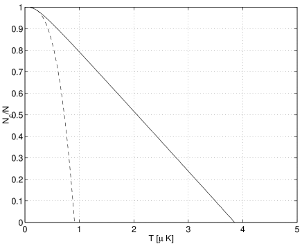
FIG. 2.: The condensate fraction as a function of temperature for $10^{6}$ sodium atoms, when $(\sigma_{x}\sigma_{y}\sigma_{z})^{1/3}=15\,\rm{\mu m}$ and trap depth $V_{1}=1\,\rm{\mu K}$. The solid line is the numerically calculated value using Eq. (7) and the dashed line is the result we get by approximating the Gaussian potential as parabolic.

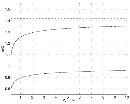
FIG. 3.: Frequencies of the collective excitations with $(n_{r}=0,l=1)$ and $(n_{r}=0,l=2)$ as a function of trap depth, for $N=10^{6}$ sodium atoms and $\sigma=15\,\rm{\mu m}$. The solid line is the exact numerically calculated value, the dashed line is the numerically calculated result for the parabolic approximation, and the dot-dashed line is based on Eq. (43). The exact result and the approximation (43) give almost the same results for most values of $V_{1}$.

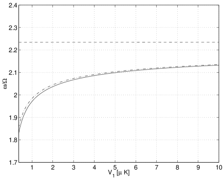
FIG. 4.: Frequency of the breathing mode $(n_{r}=1,l=0)$ as a function of trap depth for $N=10^{6}$ sodium atoms and $\sigma=15\,\rm{\mu m}$. The solid line is the exact numerically calculated value, the dashed line is the numerically calculated result for the parabolic approximation, and the dot-dashed line is based on Eq. (44).

REFERENCES

- [1] M. H. Anderson, J. R. Enscher, M. R. Matthews, C.E. Wieman, and E. A. Cornell, Science 269, 198 (1995).
- [2] C. C. Bradley, C. A. Sackett, J. J. Tollett, and R. G. Hulet, Phys. Rev. Lett. 75, 1687 (1995).
- [3] K. B. Davis, M.-O. Mewes, M. R. Andrews, N. J. van Druten, D. S. Durfee, D. M. Kurn, and W. Ketterle, Phys. Rev. Lett. 75, 3969 (1995).
- [4] D. M. Stamper-Kurn, M. R. Andrews, A. P. Chikkatur, S. Inouye, H.-J. Miesner, J. Stenger, and W. Ketterle, Phys. Rev. Lett. 80, 2027 (1998).
-
[5]
In an optical dipole trap the
potential is proportional to intensity, and the intensity of the focused
laser beam is given by
(See, for example, the review article, R. Grimm, M. Weidemüller, and Y. Ovchinnikov, e-print physics/9902072, and references therein.) In this equation is the beam waist radius and is the Rayleigh range. While the intensity distribution is not Gaussian in the direction, we expect that the results presented in this paper will give a rough estimate for the condensate properties in an optical dipole trap.(48) - [6] V. Bagnato, D. E. Pritchard, and D. Kleppner, Phys. Rev. A 35, 4354 (1987).
- [7] J. R. Ensher, D. S. Jin, M. R. Matthews, C. E. Wieman, and E. A. Cornell, Phys. Rev. Lett. 77, 4984 (1996).
- [8] S. Giorgini, L. P. Pitaevskii, and S. Stringari, J. Low Temp. Phys. 109, 309 (1997).
- [9] We have set the chemical potential to be zero, implying zero energy for the ground state of the trap. This approximation is valid only as long as the trap depth is large compared to the ground state energy.
- [10] E. Tiesinga, C. J. Williams, P. S. Julienne, K. M. Jones, P. D. Lett, and W. D. Phillips, J. Res. Natl. Inst. Stand. Technol. 101, 505 (1996).
- [11] S. Stringari, Phys. Rev. Lett. 77, 2360 (1996).
- [12] H.-J. Miesner, D. M. Stamper-Kurn, J. Stenger, S. Inouye, A. P. Chikkatur, and W. Ketterle, Phys. Rev. Lett. 82, 2228 (1999).
- [13] J. Stenger, S. Inouye, D. M. Stamper-Kurn, H.-J. Miesner, A. P. Chikkatur, and W. Ketterle, Nature 396, 345 (1998).
- [14] T.-L. Ho, Phys. Rev. Lett. 81, 742 (1998).