Phase-Induced (In)-Stability in Coupled Parametric Oscillators

Abstract

We report results on a model of two coupled oscillators that undergo periodic parametric modulations with a phase difference $\theta$. Being to a large extent analytically solvable, the model reveals a rich $\theta$ dependence of the regions of parametric resonance. In particular, the intuitive notion that anti-phase modulations are less prone to parametric resonance is confirmed for sufficiently large coupling and damping. We also compare our results to a recently reported mean field model of collective parametric instability, showing that the two-oscillator model can capture much of the qualitative behavior of the infinite system.

PACS numbers: 45.05.+x, 05.45.Xt, 05.90.+m

1 Introduction

Parametric resonance is a phenomenon pervading several fields of science. It occurs when the modulation of a system parameter causes the system to become unstable. The literature on parametric resonance is enormous, so the best one can do is cite a range of different subjects where it may play a role. Examples include mechanical systems where such resonances were first identified [1, 2, 3, 4], elementary particles [5], quantum dots [6], astrophysics [7], fluid mechanics [8], plasma physics [9], electronic networks [10], superconducting and laser devices [11], biomechanics [12], and even medicine [13]. Connections with chaotic systems have been suggested recently [14]. The simplest and perhaps most familiar example of parametric resonance occurs in a harmonic oscillator whose frequency varies periodically with time [1, 2, 3, 4]. For certain ranges of modulation parameters (frequency, amplitude) the oscillator is unstable while for others it is stable. Even for this seemingly simple system the stability boundary diagram is already quite rich and complex (see below).

A great deal of recent work has dealt with systems of coupled oscillators – again, the literature in this general area is enormous. However, very little attention has focused on systems of coupled parametric oscillators [15, 16]. Such coupled arrays are particularly intriguing because each single oscillator alone exhibits regions of stable or unstable behavior. Two questions arise naturally: 1) How does coupling modify the single-oscillator stability boundaries? 2) Are there collective parametric instabilities of the coupled system that are distinct from those experienced by single oscillators? In a recent paper Bena and Van den Broeck [15] addressed these questions for an infinite set of globally mean-field coupled harmonic oscillators subjected to time-periodic block pulses with quenched uniformly distributed random phases (“quenched” in this context means that the phase of frequency modulation of each oscillator is set at time $t=0$ and then remains unchanged). Within their mean field treatment they are able to deal with both of the questions posed above. In particular, they find wide ranges of parameter values that lead to collective instabilities.

Our interest in this paper is to identify generic coupling effects that are not specifically a consequence of the mean field analysis, and in this context to understand how a coupled system of (very) few oscillators with short-ranged interactions might carry in it the seeds of the infinite/infinitely cross-coupled array. In particular, we seek the seeds of the collective parametric instabilities. We do this by studying a model of two coupled oscillators. The control parameter in our study is the phase difference in the periodic modulation of the frequencies of the two oscillators.

In Section 2 we introduce the model and its partially analytic solution. Section 3 is a presentation of results as a large collection of stability boundary diagrams that convey the way in which stability boundaries shift, appear, and disappear with parameter changes. In Section 4 we analyze the ways in which the seeds of the collective parametric instabilities found in the mean field model already appear in the two-oscillator system. A brief summary of our conclusions is reiterated in Section 5.

2 The model

Our system consists of two linearly coupled parametric oscillators whose equations of motion are

$$\ddot{x}_{1} = -\omega_{0}^{2}[1+\phi_{1}(t)]x_{1}-k(x_{1}-x_{2})-\gamma\dot{x}_{1}$$

$$\ddot{x}_{2} = -\omega_{0}^{2}[1+\phi_{2}(t)]x_{2}-k(x_{2}-x_{1})-\gamma\dot{x}_{2}\;.$$ (1)

Here $\omega_{0}$ is the natural frequency of each (uncoupled) oscillator, $k$ is the coupling constant between them and $\gamma$ is the damping coefficient. The parametric modulations $\phi_{1}(t)$ and $\phi_{2}(t)$ are square waves with period $T\equiv 2\pi/\omega_{p}$, amplitude $A$ and phase difference $\theta$:

$$\phi_{1}(t) = A\;\mbox{sgn}\left(\sin(\omega_{p}t)\right)$$

$$\phi_{2}(t) = A\;\mbox{sgn}\left(\sin(\omega_{p}t+\theta)\right)\;.$$ (2)

With $A=0$ one is left with coupled ordinary damped harmonic oscillators whose total energy decays exponentially to zero. In the presence of the parametric modulation, however, energy is periodically pumped into the system, which may or may not lead to parametric resonance, i.e., to an infinite growth of the amplitudes of the oscillators. Our goal is to determine the boundaries between these two behaviors, which will be referred to as unstable and stable. As a point of reference we point the reader to the appendix where we review the results for a single parametric oscillator.

It is worth noting that a simple rescaling of time to dimensionless units, $t^{\prime}=t\omega_{0}$, shows that Eqs. (2) are governed by the dimensionless parameter combinations $r\equiv\omega_{0}/\omega_{p}$, $A$, $k/\omega_{0}^{2}$, $\gamma/\omega_{0}$ and $\theta$. Moreover, the behavior of the system is invariant with respect to the replacement of $\theta$ by $\theta^{\prime}\equiv 2\pi-\theta$ (reflection around $\pi$) since this just amounts to an exchange of indices between the oscillators.

2.1 Floquet theory

The linearity of the equations allows one to make use of Floquet theory to solve the problem [3]. Defining $\bm{X}\equiv(x_{1},\dot{x}_{1},x_{2},\dot{x}_{2})^{\rm T}$ where the superscript ${\rm T}$ denotes the transpose (i.e., $\bm{X}$ is a column matrix), one can rewrite Eqs. (2) in matrix form as $\dot{\bm{X}}(t)=\hat{D}(t)\bm{X}(t)$ with a matrix $\hat{D}$ satisfying $\hat{D}(t)=\hat{D}(t+T)$. Given a solution $\bm{X}(t)$ to Eqs. (2), the time periodicity of the parametric modulations thus implies that $\bm{X}(t+T)$ is also a solution. Therefore one can find a matrix $\hat{F}$ such that $\bm{X}(t+T)=\hat{F}(T)\bm{X}(t)$ and hence more generally through a repetition of this solution $\bm{X}(t+nT)=\hat{F}^{n}(T)\bm{X}(t)$. The long time behavior of the system is thus clearly determined by the eigenvalues $\{\lambda_{i}\}$ of the Floquet operator $\hat{F}$, which propagates the system in phase space for one period of the modulation. The eigenvectors $\bm{v}_{j}$ of $\hat{F}$ satisfy $|\bm{v}_{j}(t+nT)|=|\lambda_{j}|^{n}|\bm{v}_{j}(t)|$, so in the limit $n\to\infty$ parametric resonance occurs if $\max_{j}\{|\lambda_{j}|\}>1$.

The model is appealing because for any number of oscillators (a single oscillator, or the coupled oscillators considered here, or even the mean field version of an infinitely cross-coupled infinite chain [15]) the piecewise constant parametric modulation leads to a piecewise linear system whose piecewise solution is known analytically. One can therefore construct the Floquet operator explicitly by simply multiplying together piecewise linear Floquet operators. This provides an immense reduction in computational effort by skipping what is usually the most time-consuming task in obtaining the regions of parametric resonance, namely, the numerical evaluation of the Floquet operator itself. For an isolated oscillator this procedure is well known [2, 4] and reviewed in the appendix.

For the sake of clarity, let us first analyze the frictionless case $\gamma=0$. Each linear interval is characterized by one of the four possible states of the modulations $(\phi_{1},\phi_{2})=(+A,+A)$, $(+A,-A)$, $(-A,+A)$, or $(-A,-A)$. For each of these states, the solutions are of the form $X_{j}(t)=A_{j}e^{iPt}+B_{j}e^{iMt}$, where the eigenfrequencies $P$ and $M$ follow directly from the diagonalization of $\hat{D}$:

$$P^{2} = \frac{\omega_{1}^{2}+\omega_{2}^{2}+\sqrt{(\omega_{1}^{2}-\omega_{2}^{2})^{2}+4k^{2}}}{2}$$

$$M^{2} = \frac{\omega_{1}^{2}+\omega_{2}^{2}-\sqrt{(\omega_{1}^{2}-\omega_{2}^{2})^{2}+4k^{2}}}{2}\;,$$ (3)

where $\omega_{1,2}^{2}\equiv\omega_{0}^{2}[1+\phi_{1,2}(t)]+k$. Denoting the current state of the modulation by indices $+$ and $-$, notice that while $P_{++}$, $M_{++}$ and $P_{+-}=P_{-+}$ are always real, $M_{--}$ becomes imaginary when $A>1$ while $P_{--}$ and $M_{+-}=M_{-+}$ become imaginary when $A>1+2k/\omega_{0}^{2}$. Whether the system periodically alternates between harmonic behavior and one or more saddle nodes will thus depend on the parameter region and the phase difference $\theta$.

During a time interval $\tau$ with fixed $\phi_{1},\phi_{2}$ we can relate $\bm{X}(t+\tau)$ to $\bm{X}(t)$ as $\bm{X}(t+\tau)=\hat{f}(\tau)\bm{X}(t)$, where $\hat{f}$ is the piecewise linear Floquet operator:

$$\hat{f}(t)=\frac{1}{P^{2}-M^{2}}\left(\begin{array}[]{cccc}-m_{1}c_{p}+p_{1}c_{m}&-m_{1}s_{p}+p_{1}s_{m}&k[-c_{p}+c_{m}]&k[-s_{p}+s_{m}]\\ m_{1}P^{2}s_{p}-p_{1}M^{2}s_{m}&-m_{1}c_{p}+p_{1}c_{m}&k[P^{2}s_{p}-M^{2}s_{m}]&k[-c_{p}+c_{m}]\\ k[-c_{p}+c_{m}]&k[-s_{p}+s_{m}]&-m_{2}c_{p}+p_{2}c_{m}&-m_{2}s_{p}+p_{2}s_{m}\\ k[P^{2}s_{p}-M^{2}s_{m}]&k[-c_{p}+c_{m}]&m_{2}P^{2}s_{p}-p_{2}M^{2}s_{m}&-m_{2}c_{p}+p_{2}c_{m}\end{array}\right)$$ (4)

where we make use of the shorthand notation $c_{p}\equiv\cos(Pt)$, $s_{p}\equiv P^{-1}\sin(Pt)$, $c_{m}\equiv\cos(Mt)$, $s_{m}\equiv M^{-1}\sin(Mt)$, $m_{1,2}\equiv M^{2}-\omega_{1,2}^{2}$ and $p_{1,2}\equiv P^{2}-\omega_{1,2}^{2}$. The Floquet operator is then finally obtained as the product of piecewise Floquet operators with arguments that depend on the phase difference between the modulations:

$$\hat{F}(T)=\hat{f}_{-+}\left(\frac{T}{2}\frac{\theta}{\pi}\right)\hat{f}_{--}\left(\frac{T}{2}\left[1-\frac{\theta}{\pi}\right]\right)\hat{f}_{+-}\left(\frac{T}{2}\frac{\theta}{\pi}\right)\hat{f}_{++}\left(\frac{T}{2}\left[1-\frac{\theta}{\pi}\right]\right)\;.$$ (5)

The stability properties of the coupled system are determined by the magnitudes of the four eigenvalues $\lambda_{1},\dots,\lambda_{4}$ of the Floquet operator. Note that if $\theta=0$ or $\theta=\pi$, the above expression reduces to the product of only two matrices (as it should) since $\hat{f}(0)$ is just the identity matrix. The addition of damping can be dealt with by noticing that if $\bm{X}(t)$ is a solution for $\gamma=0$, then $\bm{Y}(t)\equiv e^{-\gamma t/2}\tilde{\bm{X}}(t)$ is a solution for $\gamma\neq 0$, where $\tilde{\bm{X}}(t)=\left.\bm{X}(t)\right|_{\omega_{1,2}^{2}\to\omega_{1,2}^{2}-\gamma^{2}/4}$.

3 Results

In the absence of damping, Liouville’s theorem insures that $\det\hat{f}=1$, which is confirmed by cumbersome calculations and in turn implies $\lambda_{1}\lambda_{2}\lambda_{3}\lambda_{4}=\det\hat{F}=1$. In contrast with the single oscillator (see appendix), here this is not a sufficient condition to guarantee that the parametric resonance bifurcations occur at $\lambda_{j}=\pm 1$ [2, 4]: for coupled oscillators the largest eigenvalue can cross the unit circle $|\lambda_{j}|=1$ and hence enter a region of instability (parametric resonance) in other directions in the complex plane. The fourth order characteristic polynomial needs to be solved numerically to determine the instability boundaries; this is a computationally inexpensive procedure since we have an analytic expression for the Floquet operator.

3.1 In-phase modulations

The case $\theta=0$ corresponding to in-phase modulation $\phi_{2}(t)=\phi_{1}(t)$ simplifies sufficiently to yield analytic results for the stability boundaries. This is the simplest situation to be studied, since it is possible to reduce the original four-dimensional problem in this case to two known two-dimensional systems. This decoupling is accomplished by changing the coordinate system to the reference frame of the center of mass. Defining $x\equiv(x_{1}+x_{2})/2$ and $\rho\equiv(x_{1}-x_{2})/2$, one obtains from Eq. (2)

$$\ddot{x} = -\omega_{0}^{2}[1+\phi_{1}(t)]x-\gamma\dot{x}$$ (6)

$$\ddot{\rho} = -\left\{\omega_{0}^{2}[1+\phi_{1}(t)]+2k\right\}\rho-\gamma\dot{\rho}\;.$$ (7)

Each of these equations is precisely that of a single parametric oscillator, one with frequency $\omega_{0}$ and modulation amplitude $A$, the other with rescaled parameters

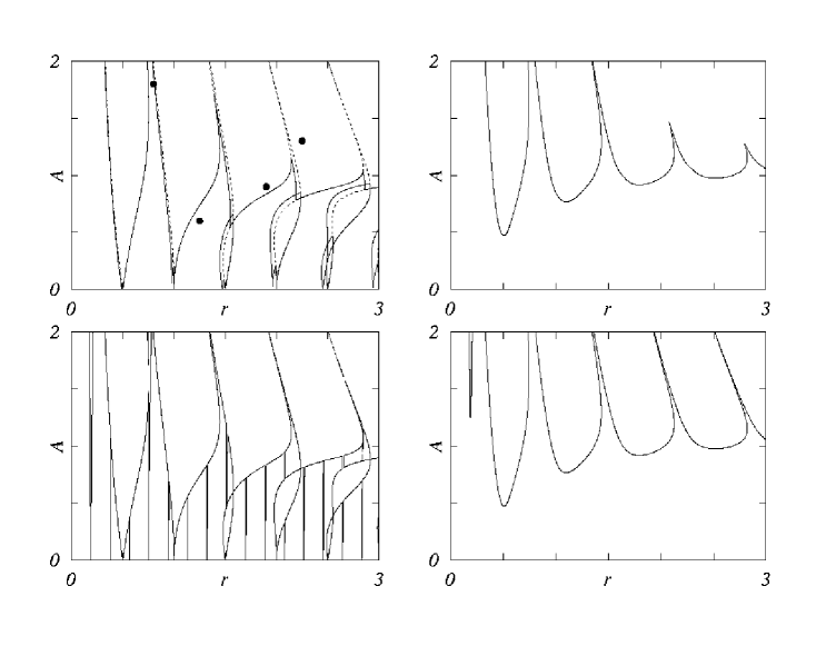
Figure 1: Instability boundaries for $\theta=0$ in the $(r,A)$ plane: $\gamma=0$ in the first column while $\gamma/\omega_{0}=0.3$ in the second column. $k/\omega_{0}^{2}=0.02$ in the first row, while $k/\omega_{0}^{2}=3$ in the second row. The dashed line in the first panel is the result for $k=0$ (single uncoupled oscillator). The dark points in this panel are parameter pairs to be considered in more detail subsequently.

$$\omega^{\prime}_{0} \equiv \sqrt{\omega_{0}^{2}+2k}$$

$$A^{\prime} \equiv A(\omega_{0}/\omega^{\prime}_{0})^{2}\;.$$ (8)

We can thus use the known results for the single oscillator [2, 4], for which a closed expression exists for the boundary of the instability regions in the $(r,A)$ plane (see the appendix).

For an undamped parametric oscillator with parameters $(r,A)$ parametric instabilities occur inside “tongues” that open up from integer and half-integer values of $r$ as discussed in the appendix and shown by the dashed curves in the first panel of Fig. 1. For the coupled problem in which we have transformed the problem to two independent parametric oscillators with different parameters, the instability regions are given by the overlap of the sets of tongues arising from each independent oscillator, one set emerging from integer and half-integer values of $r$ (“$r$-instability regions”), and the other from

$$r^{\prime}(k)\equiv r\sqrt{1+2k/\omega_{0}^{2}}=\frac{\omega_{0}^{\prime}}{\omega_{p}}$$ (9)

(“$r^{\prime}$-instability regions”). When the coupling $k$ between the oscillators is small then the two sets of tongues almost overlap and one obtains in the undamped case the solid curves in the first panel, which show the instability boundaries when $k/\omega_{0}^{2}=0.02$. Still in the undamped problem, when the coupling $k$ is large the two sets of tongues occur at different parameter scales. The boundary diagram for $k/\omega_{0}^{2}=3$ is shown in lower left panel of the figure. In either case, since now we have two independent sets of instability regions the effect of the coupling $k$ for $\theta=0$ has been to enlarge the parametric resonance regime relative to that of two uncoupled oscillators.

This last result is completely general: the effect of coupling for in-phase parametric modulations is to enlarge the parametric resonance regime relative to the uncoupled case regardless of the form of the periodic modulation. The details of the phase boundaries will of course depend on the specific modulation function.

Damping, even in an isolated parametric oscillator, destroys much of the intricate boundary structure and increases the regions of stability. This is also the case for coupled oscillators, where increasing the damping tends to blur out the effects of coupling. These behaviors can be seen in the right column of Fig. 1. The regions of instability are now restricted to larger amplitudes $A$. Note the similarity between these two figures, which involve different couplings but now with substantial damping, $\gamma/\omega_{0}=0.3$. Note also that in the lower panel of this column (large coupling) the very first instability wedge is an $r^{\prime}$-instability region while the other portions of the diagram (as well as the unstable regions in the upper weak-coupling case) include both $r$ and $r^{\prime}$ instabilities.

For the particular case $\theta=0$ these results allow us to say something about the interesting problem of asymptotic synchronization. In regions where the center of mass coordinate $x$ is unstable but the relative coordinate $\rho$ is stable ($r$-instability regions that do not overlap with $r^{\prime}$-instability regions) the coupled oscillators are synchronized if $\gamma\neq 0$ ($x_{1}=x_{2}$), that is, the two oscillators move together about the origin with ever increasing amplitude. Conversely, if $x$ is stable but $\rho$ is unstable ($r^{\prime}$-instability regions that do not overlap with $r$-instability regions), with $\gamma\neq 0$ the oscillators become “antisynchronized” ($x_{1}=-x_{2}$), that is, the two oscillators oscillate with ever increasing amplitude but in opposite directions, crossing one another each time they pass through the origin. Antisynchronization becomes more difficult to achieve with increasing coupling. If $\gamma=0$ the strict equalities $x_{1}=x_{2}$ or $x_{1}=-x_{2}$ no longer hold in the non-overlapping regions, but the difference between $x_{1}$ and $x_{2}$ or $-x_{2}$ is oscillatory and remains bounded. A simultaneous instability of both $x$ and $\rho$ involves an unstable center of mass coordinate and unbounded oscillations of each oscillator about this unbounded mean, which in turn involves a more complicated phase relation between the motions of the two oscillators. We return to this issue later.

3.2 Out-of-phase modulations

A wealth of very intricate results arises when $\theta\neq 0$. In contrast with the $\theta=0$ case, it is now no longer clear how to break down the problem into simpler independent components (even for $\theta=\pi$) and, in particular, there is no longer a transparent way to relate the results to those of single parametric oscillators.

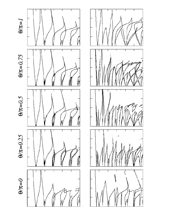
Figure 2: $(r,A)$ plane as in Fig. 1 (origin is at bottom left corner; tic marks are separated by half a unit on each axis). Left column: $k/\omega_{0}^{2}=0.05$. Right column: $k/\omega_{0}^{2}=0.5$. $\gamma=0$ for all panels.

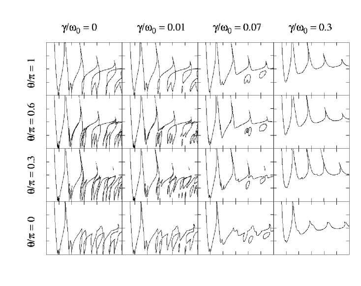
Figure 3: $(r,A)$ plane as in Fig. 1 for $k/\omega_{0}^{2}=0.12$ and several combinations of $\theta$ and $\gamma$ (origin is at bottom left corner; tic marks are separated by half a unit on each axis).

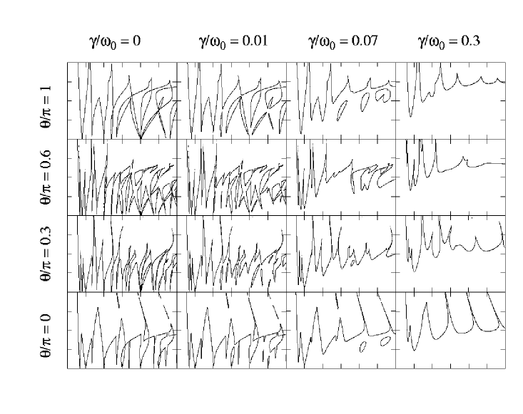
Figure 4: $(r,A)$ plane as in Fig. 1 for $k/\omega_{0}^{2}=0.6$ and several combinations of $\theta$ and $\gamma$ (origin is at bottom left corner; tic marks are separated by half a unit on each axis).

Perhaps the most striking feature of the $\theta$-dependence is its sensitivity: the unstable regions in the $(r,A)$ plane can change very abruptly (yet continuously) with the phase difference. As one might expect, this sensitivity is primarily modulated by the coupling $k$, as exemplified in Fig. 2 in the absence of damping. The left and right columns of Fig. 2 show the instability regions in the $(r,A)$ plane for $k/\omega_{0}^{2}=0.05$ and $k/\omega_{0}^{2}=0.5$, respectively. The evolution of the boundaries is shown as $\theta$ increases vertically along the columns (in order to save space, this and subsequent figures consistently omit labels, using the same scale as Fig. 1 in the $(r,A)$ plane, with the origin at the bottom left corner and tic marks separated by half a unit on both axes). While the most visible effects of the phase difference seem to concentrate on the low $A$ region for the smaller coupling (left column), the larger coupling (right column) induces a richer behavior, with (in)stabilities arising also for larger values of $A$ as $\theta$ changes. The phase difference can therefore create regions of stability and instability which are absent for in-phase modulations.

In order to address the effect of damping in this scenario, we have chosen to fix the coupling $k$ and tile several $(r,A)$ instability plots in such a way that $\theta$ varies in the vertical direction while $\gamma$ varies in the horizontal direction. Fig. 3 shows such a panel for a relatively small coupling $k/\omega_{0}^{2}=0.12$. One notices that the $\theta$ dependence is smoothed out as damping increases, so that almost no structure is visible along the rightmost column ($\gamma/\omega_{0}=0.3$). Fig. 4 shows the results for a larger coupling $k/\omega_{0}^{2}=0.6$. Note that the same tendency is observed: the instability boundaries become gradually less sensitive to $\theta$ as $\gamma$ increases. However, the rightmost column of Fig. 4 now shows much more structure than that of Fig. 3, indicating that for the same value of $\gamma$, the $(r,A)$ plane with larger $k$ shows a stronger $\theta$ dependence.

Figs. 3 and 4 suggest that $\theta=\pi$ gives rise to particularly stable behavior. This is in agreement with the vague intuitive notion that anti-phase modulations should be less prone to resonance than in-phase ones. In order to verify the extent to which this intuition is correct, a complementary view of these phenomena can be obtained by projecting the instability regions in the $(k,\theta)$ plane instead. This allows us to start with uncoupled oscillators ($k=0$) and observe how a given (in)stability evolves as $k$ and $\theta$ change. Indeed, it turns out to be possible to understand much of the behavior of the coupled system in terms of the behavior of the uncoupled system. To produce the representative results shown in Figs. 5 and 6, we fix several $(r,A)$ points in the single oscillator stability boundary diagram shown as black circles in the first panel of Fig. 1 and study the way in which variations in $k$ and $\theta$ affect these particular states. Two of the points in Fig. 1, $(r,A)=(0.8,1.8)$ and $(1.25,0.6)$ are stable states for the single oscillator (the first black dot touches the stability boundary in the figure only because it has been drawn large enough to render it visible; the point is well within the stable region). The other two points, $(r,A)=(1.9.0.9)$ and $(2.25,1.3)$ lead to unstable behavior of the single oscillator.

The first thing to be noted in Fig. 5 is that the horizontal axis has been rescaled in order to reveal the relevance of the variable $r^{\prime}$ (see Eq. (9)). The top panels focus on $r=1.9$ and $A=0.9$, which is in the parametrically resonant regime for the uncoupled system. The small-$r^{\prime}$ portion of the figure thus represents an unstable regime. One notes that for $r^{\prime}(k)$ slightly above 2 the system becomes stable within a $\theta$ interval centered around $\pi$. Increasing $k$ a little further, this stability region then evolves in a very complex pattern, which includes reentrant “holes” of instability. After a distinguishable gap of instability, a somewhat simpler band of stability arises around $r^{\prime}\sim 3.5$ starting at $\theta=\pi$. This band continues to larger values of $k$, with its outermost boundaries presenting a relatively simpler envelope than the low-$k$ pattern. The interesting point to be emphasized is that the band is perforated by gaps of instability most of which are centered precisely at integer and half-integer values of $r^{\prime}$. This result is perhaps anticipated by the fact that the frequency $\omega_{0}^{\prime}$ appears as the effective average diagonal frequency in the mean field equation of motion in [15]). The gaps are eventually closed by increasing the damping (top right panel), which also broadens the stability band and simplifies its dependence on the phase difference. The bottom panels in Fig. 5 are for $r=2.25$ and $A=1.3$, which again is in the resonant regime of the single oscillator. One notices the same pattern: for lower values of $k$, a complex shape emerges in the $\theta$ dependence of the stable regions. For sufficiently large values of $k$, a band of stability arises which has instability gaps basically centered at integer and half-integer values of $r^{\prime}$. Damping (bottom right panel) causes gaps to disappear, creating a uniform region of stability centered around $\theta=\pi$.

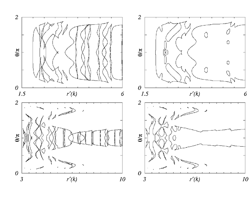
Figure 5: Stability regions in the $(k,\theta)$ plane in the absence (left column, $\gamma=0$) or presence (right column, $\gamma/\omega_{0}=0.05$) of damping. Top panels: $r=1.9$ and $A=0.9$. Bottom panels: $r=2.25$ and $A=1.3$.

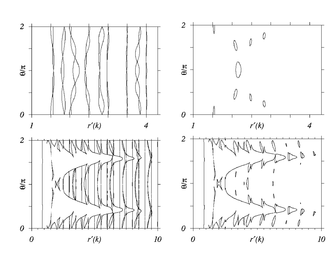
Figure 6: Instability regions in the $(k,\theta)$ plane in the absence (left column, $\gamma=0$) or presence (right column, $\gamma/\omega_{0}=0.05$) of damping. Top panels: $r=1.25$ and $A=0.6$. Bottom panels: $r=0.8$ and $A=1.8$.

Fig. 6 presents what may be regarded as the opposite situation, namely, when the original uncoupled system is stable. The top panels show the results for $r=1.25$ and $A=0.6$. Notice that the behavior is much simpler in this case, with the original stability being disturbed mostly around integer and half-integer values of $r^{\prime}$ in the absence of damping (top left), with a relatively weak $\theta$ dependence. The effect of damping (top right) is to suppress most of these instability regions, yielding a predominantly stable $(k,\theta)$ plane. The bottom panels show results for an interesting intermediate situation: even though the uncoupled system is stable for $r=0.8$ and $A=1.8$, this point lies in a narrow corridor between two instability regions in the $(r,A)$ plane (see Fig. 1). One would therefore expect instabilities to arise more easily, and the immediate question is how the resulting diagram might reconcile the structures observed in Fig. 5 and the top panels of Fig. 6. The answer lies in a very rich structure in the $(k,\theta)$ plane (bottom left panel): initially, very small coupling induces an instability for all $\theta$. The now predominantly unstable system evolves in a manner similar to those of Fig. 5, a stability region being created around $\theta=\pi$ as $k$ increases, with string-like gaps of instability around the usual values of $r^{\prime}$. The difference is that there is now also a second band of stability centered around $\theta=0$, presenting gaps at the same $r^{\prime}$ positions. For $k$ sufficiently large, those two stability bands merge and one is left with a structure similar to that of the top panels: a predominantly stable region permeated by strings of instability. The bottom right panel of Fig. 6 shows the effect of damping, which significantly reduces the instability gaps thus greatly simplifying the picture.

Therefore the notion that modulations operating with a phase difference $\theta=\pi$ are less prone to parametric resonance is thus seen to be essentially correct. Framing this statement more carefully, our results show that for given $r$ and $A$, sufficiently large values of $k/\omega_{0}^{2}$ and $\gamma/\omega_{0}$ are able to induce, in the $(k,\theta)$ plane, a band of stability centered around $\theta=\pi$ even if the uncoupled oscillators are individually unstable. The width of this band can eventually comprise the whole $2\pi$ interval if the uncoupled system is originally stable.

4 Collective parametric instability

Bena and Van den Broeck [15] studied the stability boundaries of $N$ parametrically modulated oscillators $\{x_{i}\}$ each coupled to all the others by the same coupling constant $2k/N$ (in our notation). The phases $\{\theta_{i}\}$ are initially chosen at random from a uniform distribution in the interval $[0,2\pi]$, remaining quenched thereafter. With square-block modulation the system is exactly solvable in the limit $N\to\infty$, where the mean-field solution becomes exact. The mean field equation is

$$\ddot{x}=-\omega_{0}^{2}[1+\phi_{\theta}(t)]x-\gamma\dot{x}-2k(x-\left<x\right>)$$ (10)

where $x$ is the displacement of any oscillator in the chain, $\phi_{\theta}(t)$ is the periodic modulation with phase $\theta$, and $\left<x\right>\equiv N^{-1}\sum_{i=1}^{N}x_{i}$ is the mean displacement to be determined self-consistently. Bena and Van den Broeck note that the exact solution of this equation is

$$\left(\begin{array}[]{c}x(t)\\ \dot{x}(t)\end{array}\right)=\mathbf{G}_{\theta}(t)\cdot\left(\begin{array}[]{c}x(0)\\ \dot{x}(0)\end{array}\right)+2k\mathbf{G}_{\theta}(t)\cdot\int_{0}^{t}d\tau\mathbf{G}_{\theta}(\tau)^{-1}\cdot\left(\begin{array}[]{c}0\\ \left<x(\tau)\right>\end{array}\right)\;.$$ (11)

The propagator $\mathbf{G}(t)$ is known explicitly. Indeed, at $t=T$ it is $\mathbf{G}(T)=e^{-\gamma T}\hat{F}(T)$ where $\hat{F}$ is precisely the single-oscillator Floquet operator given in Eqs. (A.9) and (A.10), but now with the frequencies shifted by the coupling constant

$$\omega_{\pm}=\sqrt{\omega_{0}^{2}(1\pm A)+2k-\gamma^{2}/4}.$$ (12)

Note that this is exactly the same as the propagator associated with the $\rho$ variable of Eq. (7) in the two-oscillator in-phase modulation problem, that is, the propagator associated with a single oscillator of frequency $\omega_{0}^{\prime}$.

Bena and Van den Broeck identify two sorts of instabilities. One, which they call the “usual parametric resonance,” arises from the divergence associated with eigenvalues of $\mathbf{G}$ of magnitude greater than unity, that is, with the unbounded growth of the first term in Eq. (11) which in turn signals the unbounded growth of the amplitude of any typical oscillator in the chain. The stability boundaries associated with this type of instability are given precisely by Eq. (A.12) and are shown for the parameter choices indicated in the caption as the dotted curves in the top row panels of Fig. 7. In our in-phase two-oscillator parlance these are exactly the boundaries of the “$r^{\prime}$-instability regions” defined in terms of the shifted frequency $\omega_{0}^{\prime}$ (cf. Eq. (3.1)). The “usual” regions shrink in width and move toward lower $r$ and larger $A$ with increasing coupling $k$, a behavior already exhibited in the context of the in-phase two-oscillator results of Fig. 1. Indeed, this instability is beyond the scale of the figures in the large-coupling bottom row panels. The other type of instability, which they call a “collective instability,” is associated with the divergence of the mean $\left<x\right>$ and hence of the second term in Eq. (11). The collective instability boundaries are shown as dashed curves in all panels of Fig. 7. Note that the two types of instabilities may occur simultaneously, as seen in the instability region overlap evident in the top row panels of the figure. We return to this point below. Note also that with increasing coupling the system becomes increasingly stable, as one might expect, and that the unstable behavior becomes primarily collective.

Figure 7: Instability regions in the $(r,A)$ plane for $\gamma/\omega_{0}=0.4$. According to the mean field model [15], usual parametric resonance occurs inside the dotted boundaries, while the boundaries of collective instability are depicted by dashed lines. $k/\omega_{0}^{2}=4$ for the top panels, and $k/\omega_{0}^{2}=20$ for the bottom panels. The thin solid lines correspond to $k=0$ (left column); the thick solid lines (right column) correspond to $\theta=\pi$ in the two-oscillator model. The dark points in the upper right panel are parameter pairs considered in more detail subsequently.

We wish to explore whether our two-oscillator model is able to capture at least some of the behavior of the infinite system. In particular, we would like to investigate whether features of the collective instabilities of the mean field model are apparent in a system of only two oscillators with a fixed relative modulation phase. To make the comparison we also show in Fig. 7 the stability boundary for a single uncoupled oscillator (thin solid lines in left column) and for coupled oscillators with relative modulation phase $\theta=\pi$.

We make the following assertions: the two-oscillator system with any value of $\theta$ captures features of the overlap region of “usual” and “collective” instabilities. The purely “usual” regions are captured most accurately by the $\theta=0$ system, and the purely “collective” regime is best captured by the two-oscillator system with $\theta=\pi$. It is therefore this latter system that most fully captures (with unexpected detail) the principal features of collective behavior of the mean field model, and does so with increasing accuracy as the coupling between oscillators increases. We support these assertions, particularly the last one which is the one of most interest to us, with the results shown in Figs. 7 and 8.

Clearly, the $\theta=0$ system captures the full “usual” instability regime exactly since, as already stated, the “usual” instability is exactly the same as the “$r^{\prime}$-instability.” This identity is not restricted to the square wave modulation but holds for any periodic modulation. However, the $\theta=0$ system does not capture the “collective” instability since the “$r$-instability” condition is that associated with a single parametric oscillator with the unshifted frequency $\omega_{0}$. Thus, for example, in the first panel of Fig. 7 the $\theta=0$ instability boundaries can be constructed from the combination of the dotted regimes and the thin solid lines (compare with the right lower panel of Fig. 1), whereas those of the mean field system include the same dotted regimes but now the very different dashed regions. The left lower panel shows an even greater difference between the $\theta=0$ two-oscillator model (whose “$r$-instability” boundaries are independent of $k$) and the mean field model (where the boundaries of the collective instability are sensitively dependent on $k$). Two coupled parametric oscillators with relative modulation phase $\theta=0$ therefore do not capture the collective features of the mean field model.

Our assertion that the two-oscillator system with any $\theta$ contains elements of the “usual” instabilities in the mean field model is simply a restatement of our earlier observation that “$r^{\prime}$-instabilities” continue to appear even when one moves away from $\theta=0$ and all the way to $\theta=\pi$.

Consider now the two coupled oscillators with $\theta=\pi$. The stability boundaries are shown by the thick solid lines in the panels in the right column of Fig. 7. In the upper panel we observe that the first tongue approximates the region of “usual” mean field instability (in the non-overlapping regime) and that the remainder captures the collective instability boundary features surprisingly well (although it does miss the gap). We particularly point to the excellent fit of the leftmost boundary of this region. The agreement between the two models is even more dramatic in the lower panel, which corresponds to stronger coupling $k$. Again, the details are surprisingly well matched and the leftmost boundary of the region is captured essentially exactly.

To further support our analysis, and to gain a clearer understanding of the difference between “usual” and “collective” instabilities (which are both evidently already present in our two-oscillator system although the notion of a collective effect is not obvious in such a small system), we consider the motions that might characterize the instabilities. In the mean field system we conjecture that in the non-overlapping “usual” instability regime the mean is zero, $\left<x\right>=0$, but each oscillator oscillates about zero with ever increasing amplitude. The motion in the non-overlapping “collective” instability regime may involve an ever increasing mean with each oscillator oscillating about this moving mean with finite amplitude. This description is in accord with that of Bena and Van den Broeck [15]. The overlap regions may involve both an increasing mean and oscillations of ever increasing amplitude about the moving mean. We have not ascertained these conjectures in the mean field system, but present results for the two-oscillator system that support this description.

Figure 8: Trajectories for the two-oscillator $\theta=\pi$ system for the parameters corresponding to the dark points in the upper right panel of Fig. 7: $\gamma/\omega_{0}=0.4$, $A=3$, and $k/\omega_{0}^{2}=4$. $r=0.25$ in the upper panel and $0.4$ in the lower panel. The dashed curves are the displacement $x_{1}$ of one oscillator vs time, the dotted curves are the displacement $x_{2}$ of the other oscillator, and the thick solid curves represent the mean displacement $x=(x_{1}+x_{2})/2$.

Figure 8 shows trajectories for the two-oscillator $\theta=\pi$ system at the two points marked on the upper right panel of Fig. 7. The trajectories shown are those of each of the two oscillators as well as the mean trajectory. The upper panel is for parameter values in the unstable region that is not in the “collective” regime. It is tempting to associate this with the non-overlapping “usual” instability of the mean field model, an association that requires some caution. The figure indicates that not only does each oscillator and also the mean oscillate about zero, but all the trajectories, including the mean, appear to diverge. This behavior is that envisioned in our earlier discussion of the $\theta=0$ two-oscillator system in the regime where “$r$-instabilities” and “$r^{\prime}$-instabilities” overlap, and is an indication that features of both kinds of instabilities persist even at $\theta=\pi$. We conjecture that “$r$-instabilities” are finite size divergences not present in the mean field model (and hence we would not expect to see this particular type of trajectory there). In the mean field limit only the “$r^{\prime}$-instability” contributions in this regime persist, becoming the non-overlapping “usual” instability portion of the phase boundary portrait.

The lower panel of Fig. 8 is for parameter values in the non-overlapping “collective” regime. The mean indeed increases, and each oscillator oscillates about this increasing mean. It is interesting that the main feature of the “collective” instability, namely, an increasing mean displacement with individual oscillators oscillating about this mean, is already clearly captured by the two-oscillator model.

5 Conclusions

We have presented results for a model of two coupled parametric oscillators that can be solved for any value of the phase difference $\theta$ between the modulations. The other parameters of the problem are the oscillator frequency $\omega_{0}$, the modulation amplitude $A$ and period $T=2\pi/\omega_{p}$, the coupling $k$ and the damping $\gamma$.

We found that in-phase ($\theta=0$) coupled oscillator motion can be separated into two independent contributions. One involves the two oscillators moving together about zero (“$r$-instabilities”). The instability boundaries for this motion are identical to those of a single parametric oscillator of frequency $\omega_{0}$ and are independent of coupling $k$ since the spring connecting the oscillators is never disturbed. The other involves the two oscillators moving about zero but exactly in anti-phase with one another (“$r^{\prime}$-instabilities”). The stability boundaries are sensitive to $k$ for these motions: the system becomes more stable with increasing coupling. We noted that these latter instabilities are exactly those identified as “usual” instabilities in the mean field model [15] and that they contribute to the instability boundaries in our two-oscillator model for any $\theta$, not just for $\theta=0$. We also showed that damping shrinks the instability regimes and smoothes the stability boundaries.

We showed that a change in $\theta$ can substantially modify the regions of parametric instability as projected in the usual $(r=\omega_{0}/\omega_{p},A)$ plane, and that these changes are strongly affected by the coupling between the oscillators. In general, increasing $\theta$ up to $\pi$ provides greater stability but also leads to more intricate stability boundaries. An increase in $k$ and/or $\gamma$ also leads to increased stability. Alternatively, it is possible to understand the coupled system in terms of the uncoupled system by projecting the instability regions onto the $(k,\theta)$ plane. This rendition is particularly useful to show that $\pi$-centered bands of stability arise for sufficiently large $k$ and $\gamma$. We have thus identified all the trends of behavior in the two-oscillator model as each of the parameters is varied.

Our most interesting insights arise from a comparison of the two-oscillator results with the mean field model [15] consisting of $N\rightarrow\infty$ parametrically modulated oscillators all coupled to one another. In this latter system two types of instabilities have been identified: “usual” and “collective.” The “usual” instabilities are exactly our “$r^{\prime}$-instabilities,” that is, the stability boundaries are identical. The interesting result is that the “collective” instabilities already appear in the two-oscillator model with $\theta=\pi$. This statement is based on the great similarity of the stability boundaries of the mean field and two-oscillator systems, especially with increasing coupling, and the specific features of the oscillator trajectories that typify the motions in each of these unstable regimes. It is perhaps surprising that a two-oscillator model can capture so much of the mean field collective behavior, and suggests that collective resonance in the latter may be dominated by phases quenched around $\pi$.

APPENDIX A - Parametric Resonance for a Single Oscillator
A brief review of parametric resonance for a single oscillator provides results called upon in the body of the paper for the coupled system [2, 4]. The equation of motion is

$$\ddot{x}+\omega^{2}(t)x+\gamma\dot{x}=0\;.$$ (A.1)

The frequency $\omega(t)$ is a periodic function with period $T\equiv 2\pi/\omega_{p}$. The simplest model of such a parametric modulation is perhaps the square wave

$$\omega^{2}(t)=\omega_{0}^{2}\left[1+A\mbox{sgn}(\sin(\omega_{p}t))\right]\;.$$ (A.2)

In the undamped case ($\gamma=0$) the oscillator frequency thus switches periodically between the two values $\omega_{\pm}=\omega_{0}\sqrt{1\pm A}$. If $A\leq 1$, the system jumps between two oscillatory regimes, each of which is stable. If $A>1$, then $\omega_{-}$ becomes purely imaginary, corresponding to a saddle node behaviour in the phase space $(x,\dot{x})$. In this case, the system jumps between an unstable saddle and a stable oscillatory regime. As we shall see below, both instability and stability can occur for either $A\leq 1$ or $A>1$. With damping, the relevant frequencies are shifted (see below). The stability of the system depends on the interplay between the amplitude $A$ of the modulation and its frequency $\omega_{p}$ as well as the system parameters $\omega_{0}$ and $\gamma$.

The linearity of the equations leads naturally to the application of Floquet theory for the solution of the problem [3]. A change of variables to

$$y(t)=e^{\gamma t/2}x(t)$$ (A.3)

yields the undamped equation

$$\ddot{y}+\tilde{\omega}^{2}(t)y=0\;$$ (A.4)

where

$$\tilde{\omega}^{2}(t)=\omega^{2}(t)-\frac{\gamma^{2}}{4}.$$ (A.5)

For the square wave modulation we then have

$$\tilde{\omega}=\left\{\begin{array}[]{l}\tilde{\omega}_{+}\equiv\sqrt{\omega_{0}^{2}(1+A)-\gamma^{2}/4}\\[12.0pt] \tilde{\omega}_{-}\equiv\sqrt{\omega_{0}^{2}(1-A)-\gamma^{2}/4}\end{array}\right.$$ (A.6)

Due to the periodicity of $\tilde{\omega}(t)$ the two independent solutions of Eq. (A.4) must also have period $T$. One can write for the original variable

$$\mathbf{X}(t+T)=e^{-\gamma T}\hat{F}(T)\mathbf{X}(t)\;,$$ (A.7)

where

$$\mathbf{X}\equiv\left(\begin{array}[]{c}x\\ \dot{x}\end{array}\right)$$ (A.8)

and $\hat{F}$ is the so-called Floquet operator that (aside from damping) propagates the system in phase space for one period:

$$\hat{F}(T)=\hat{f}_{-}\left(T/2\right)\hat{f}_{+}\left(T/2\right)\;.$$ (A.9)

where

$$\hat{f}_{\pm}(t)=\left(\begin{array}[]{cc}\cos\tilde{\omega}_{\pm}t+\frac{\gamma}{2\tilde{\omega}_{\pm}}\sin\tilde{\omega}_{\pm}t&\frac{1}{\tilde{\omega}_{\pm}}\sin\tilde{\omega}_{\pm}t\\[12.0pt] \-\frac{\omega_{\pm}^{2}}{\tilde{\omega}_{\pm}}\sin\tilde{\omega}_{\pm}t&\cos\tilde{\omega}_{\pm}t-\frac{\gamma}{2\tilde{\omega}_{\pm}}\sin\tilde{\omega}_{\pm}t\end{array}\right)$$ (A.10)

Equation (A.7) implies that

$$\mathbf{X}(t+nT)=e^{-n\gamma T}\hat{F}^{n}(T)\mathbf{X}(t)\;,$$ (A.11)

so the long term behavior of the system is governed by the eigenvalues of $e^{-\gamma T}\hat{F}$. If any eigenvalue is larger than 1 in absolute value, there is parametric resonance and the system is unstable.

One can show that the two eigenvalues of $e^{-\gamma T}\hat{F}(T)$ obey the relation $\lambda_{1}\lambda_{2}=1$, reflecting the incompressible piecewise Hamiltonian flow. Therefore the eigenvalues are complex conjugates in the stable regions and real in the unstable regions. At the boundaries both eigenvalues equal either $+1$ or $-1$, in which case the system oscillates with period $T$ or $2T$, respectively. Therefore the trace of the Floquet operator is $\pm 2$ at the stability boundaries, leading to the following boundary equation:

$$\cos\left(\frac{\tilde{\omega}_{-}T}{2}\right)\cos\left(\frac{\tilde{\omega}_{+}T}{2}\right)-\left(\frac{\tilde{\omega}_{+}^{2}+\tilde{\omega}_{-}^{2}}{2\tilde{\omega}_{+}\tilde{\omega}_{-}}\right)\sin\left(\frac{\tilde{\omega}_{-}T}{2}\right)\sin\left(\frac{\tilde{\omega}_{+}T}{2}\right)=\pm\cosh\left(\frac{\gamma T}{2}\right)\;.$$ (A.12)

In the absence of damping the solutions depend only on $A$ and the ratio $r\equiv\omega_{0}/\omega_{p}$, and these particular results are shown by the dashed curves in the first panel of Fig. 1. The regions of instability appear as “tongues” starting from integer and half-integer values of $r$ at small modulation amplitudes. Note that the stability boundaries surrounding the tongues that emerge from integer values of $r$ correspond to both Floquet eigenvalues being equal to $1$, while those surrounding tongues that emerge from half-integer values of $r$ are associated with the Floquet eigenvalues equal to $-1$. Note that no abrupt transition (nor a visible transition of any kind) is seen at the line $A=1$ which marks the transition between an oscillating-oscillating behavior and a saddle-oscillating one. As one would expect, on the other hand, the system is nearly always unstable for sufficiently small $\omega_{p}$ and sufficiently large $A$ (upper right corner of the figure).

Acknowledgements:

We would like to thank C. Van den Broeck and R. Kawai for stimulating discussions. This work was supported in part by the National Science Foundation under grant No. PHY-9970699.

References

- [1] L. D. Landau and E. M. Lifschitz, Mechanics (Pergamon Press, Oxfors, 1969).
- [2] V. I. Arnold, Equations Différentielles Ordinaires (Editions Mir, Moscou, 1974); English translation: Ordinary Differential Equations (Springer-Verlag, Berlin, 1992); Mathematical Theory of Classical Mechanics (Springer-Verlag, Berlin, 1989).
- [3] A. H. Nayfeh and D. T. Mook, Nonlinear Oscillations (Wiley, New York, 1979).
- [4] C. Van den Broeck and I. Bena, “Parametric resonance revisited,” preprint.
- [5] E. Kh. Akhmedov, J. Physics 54, 47 (2000).
- [6] M. Calvo, Phys. Rev. B 60, 10953 (1999).
- [7] I. Zlatev, G. Huey and P. J. Steinhardt, Phys. Rev. D 57, 2152 (1998).
- [8] J. W. Miles, J. Fluid Mech. 148, 451 (1984); S. T. Milner, J. Fluid Mech. 225, 81 (1991).
- [9] S. Riyopoulos, J. Plasma Phys. 46, 473 (1991); Phys. Rev. Lett. 68, 3303 (1992).
- [10] M. Calvo, Phys. Rev. B 55, 10571 (1997).
- [11] N. V. Fomin, O. L. Shalaev and D. V. Shantsev, J. Appl. Phys. 81, 8091 (1997); K. Otsuka, D. Pieroux, W. Ting-Yi and P. Mandel, Optics Lett. 22, 516 (1997).
- [12] M. Schienbein and H. Gruler, Phys. Rev. E 56, 7116 (1997); F. S. Prato, M. Kavaliers, A. P. Cullen and A. W. Thomas, Bioelectromagnetics 18, 284 (1997).
- [13] D. Ballon et. al., Magnetic Resonance in Medicine 39, 789 (1998).
- [14] R. Kobes and S. Peleš, nonl-phys 0005005 (2000).
- [15] I. Bena and C. Van den Broeck, Europhys. Lett. 48, 498 (1999).
- [16] J-Y. Ji and J. Hong, J. Phys. A 31, L689 (1998).