A nonlinear hydrodynamical approach to granular materials

Abstract

We propose a nonlinear hydrodynamical model of granular materials. We show how this model describes the formation of a sand pile from a homogeneous distribution of material under gravity, and then discuss a simulation of a rotating sandpile which shows, in qualitative agreement with experiment, a static and dynamic angle of repose.

I Introduction

The nature of the theory which describes the macroscopic transport in granular materials overview remains an unsolved problem. We propose here a candidate theory, inspired by features of nonlinear hydrodynamics (NH). Given its success in treating transport in a variety of complex systems NH , NH seems natural to use in this context. In developing any continuum model of granular materials, however, one is challenged by the need to incorporate some remnant of the discrete nature of the underlying material.

The development of our theory is based on the hypothesis that the states of a system can be specified in terms of a few collective variables (at sufficiently long length scales), and that these states are connected in time by the local conservation laws supplemented with constituitive relations. Typically, the collective variables used are the conserved densities which, in the simplest view of granular materials, are conservation of mass and momentum. Conservation of energy is more complicated in this case than in simple fluids, due to locally inelastic processes collapse which may transfer energy into internal degrees of freedom. Although we know how to include the energy density into the description, we begin with a more primitive theory which uses only the mass density $\rho$ and the momentum density $\vec{g}$.

The key difference between simple fluids and granular materials is that fluids organize over short time scales to be spatially homogeneous, while granular materials can exist over very long times in spatially inhomogeneous metastable states: metastable, because individual grains do not always pack together efficiently; long-lasting, because the large masses of the grains prevent thermal fluctuations from adjusting particles into a tighter configuration. Any complete description of granular materials must be able to explain the nature of these quenched inhomogeneous states. Experiment suggests that a sandpile contains “force chains” forcechains which serve to support the pile in the presence of external stress; these chains are surrounded by regions of sand which are comparatively unstressed, and which allow the pile to flow and to settle under vibrations.

Since these sandpiles (in the absence of forcing) are static, the momentum is negligible, and we are left with the density field as our sole tool in describing the pile. Our primary hypothesis is that the density field alone is sufficient to capture the metastable nature of the system when at rest. Specifically, we describe the force chains as regions of sand in which the packing of the grains is ideal, having the maximum possible density. We will call these regions “close-packed”. The other, “loose-packed” regions have their grains arranged in some non-optimal configuration, with a slightly smaller density. We propose that these small variations in the density field are sufficient to describe the metastable nature of sand.

Using dynamical equations based on local conservation of mass and momentum, this quenched pattern in the density can be prepared in a dynamic process driven by an effective free energy with minima characterizing the loose-packed and close-packed regions. This presents the opportunity to grow a sand pile under the influence of gravity starting from an initial homogeneous state, and in the construction of the sand pile one builds up, in a self-consistent manner, an inhomogeneous equation of state characterized by a nontrivial stress tensor.

The basic structure of our theory, based on local conservation laws, is straightforward. More difficult is the inclusion of these competing close and loose-packed states. Clearly these require a detailed description of the shortest length scales treated in the model; there is a competition of length and energy scales of a type not encountered in simple fluids. Such a short-range description will depend on details of the particular granular material; we will be satisfied with a theory that demonstrates some generic properties of sand, as described in the next section. It seems reasonable that one may then be able to refine the model to include variations in the shapes and types of individual grains.

While the short-range length scales give difficulty, the large-scale nature of our model presents us with the advantage of a description close in scale to those phenomena which are most visible to experiment and casual observation. One ultimate goal is to address the existing Knight macroscopic shaking and rotation experiments. Also, such a theory should eventually be useful in analyzing the surface states produced in large-amplitude shaking experiments surfacestates .

There have been a number of attempts Hydro to use hydrodynamics to understand the dynamics of sand piles. These efforts differ from the one advanced here in that they do not propose to follow the full evolution of the system. There has also been a significant theoretical effort to describe granular materials through the use of kinetic theory kinetictheory . This approach is organized at a more microscopic level, where the connection to the macroscopic, static, metastable phase of the system is less direct foot-kinetic and coupling to experiment more difficult. In many of these cases it is necessary to “liquefy” the granular material in question, giving it so much energy that it loses its metastable quality which seems to be crucial in describing certain aspects of a sandpile’s behavior.

In this paper we begin by describing some generic features of sand which we hope to incorporate into our model. We then proceed to a development of our dynamical equations from a generalized Langevin equation. This will lead into a discussion of the choice of a driving free energy, which will be crucial in creating the quenched pattern in the density field.

To test the validity of the theory we turn to simulation on a two-dimensional lattice. We begin with a rectangular box containing a homogeneous distribution of sand under the influence of gravity, and we show that it does indeed form a sand pile with an inhomogeneous distribution of loose and close-packed states. We then turn to simulations in a circular container, first forming a sand pile using the same technique, and then rotating the pile at different speeds. We compare the resulting angles of repose and oscillations about those angles to corresponding experimental data in the literature.

II Properties of Granular Materials

We want to construct our model to be compatible with the following aspects of granular materials:

1. Granular materials have a clumping property; simulations of simple systems of inelastically colliding balls provide evidence for this phenomenon. One possible explanation for this clumping is the theory of inelastic collapse collapse : when two particles collide inelastically, they lose energy from their translational degrees of freedom and so recede more slowly than they approach each other. On average, the particles stay closer together than if they had collided elastically, and regions of higher density build up. This can also be described in terms of a hydrodynamical instability Goldhirsch .

2. Thermal energies in a sand pile are very small compared to, for instance, the average gravitational energy. Thus we should be able to ignore thermal noise.

3. Because of the large masses of the grains, one does not expect a significant vapor pressure above the interface as is found in liquid-gas systems. Indeed we expect a very dilute gas of grains above the pile, whose density exhibits a Boltzmann distribution due to the effect of gravity.

4. Sand piles are strongly driven by gravity and, because of the lack of thermal effects, the dense sand pile is separated from the dilute gas above by a sharp interface.

5. Granular materials are strongly disordered, with metastable structures forming upon creation of a pile. This is also due to the lack of thermal effects. As mentioned in the introduction, there is evidence of stress chains running through the bulk of sand piles, which may be associated with the ramified clumps formed in the more dilute systems studied using kinetic theory. The important point for us is that there is competition between somewhat more dense domains (stress chains and arches) and other, more loosely-packed regions in the pile.

6. Granular materials are stiff: when moved or jostled the pile can for a time behave as a solid object. Thus the sand pile should have a relatively uniform density.

7. One specific example of this stiffness is that a sand pile can maintain a non-horizontal surface. For example, when a pile of sand in a container is rotated about a horizontal axis, it does not flow immediately but waits until its surface passes a certain critical angle (called the angle of repose) with the horizontal. According to Reynolds Reynolds , this effect is due to the static interlocking grains that make up a granular material: the pile must dilate first, giving these grains freedom to move about, before flow is possible.

8. It is well known that granular materials can be very sensitive to boundary and finite-size effects; the famous Brazil-nut-to-the-top phenomenon Brazil-nut , for instance, is strongly influenced by both.

We will touch on these points while developing our model.

III Dynamical Equations

Inspired by nonlinear hydrodynamics, we begin with the generalized Langevin equation Ma ; Das

$$\frac{\partial\psi_{\alpha}(\vec{x},t)}{\partial t}=V_{\alpha}[\psi(\vec{x},t)]-\Gamma_{\alpha\beta}(\vec{x}){\delta F[\psi(\vec{x},t)]\over\delta\psi_{\beta}(\vec{x},t)}.$$ (1)

(Throughout this section, summation is implied over all repeated indices.) The variables $\psi_{\alpha}$ are the “slow” fields of interest in the problem: as mentioned earlier, these are the density field $\rho(\vec{x})$ and the momentum field $\vec{g}(\vec{x})$. The first term $V_{\alpha}[\psi]$ is the streaming velocity, and corresponds to the reversible terms in typical hydrodynamical equations. As we will see, it depends on the Poisson brackets of the slow fields, as well as the derivatives of the Landau-Ginzburg-Wilson (LGW) effective free energy $F$. The second term is dissipative in nature, and $\Gamma_{\alpha\beta}$ is the symmetric matrix of dissipative coefficients. Because granular materials are essentiallly zero-temperature systems (property 2), there is no thermal noise driving the system.

For our system, the free energy $F$ can be broken up into kinetic, potential, and external parts:

$$F=F_{K}+F_{P}+F_{E}.$$ (2)

From thermodynamics, one has the result that the variable conjugate to the momentum density is the velocity field:

$${\delta F\over\delta g_{i}(\vec{x})}\equiv v_{i}(\vec{x})\equiv{g_{i}(\vec{x})\over\rho(\vec{x})},$$ (3)

where $i$ is a vector label. The kinetic energy contribution to the free energy thus has all of the momentum dependence:

$$F_{K}=\int d^{d}\vec{x}\,{\vec{g}^{2}(\vec{x})\over 2\rho(\vec{x})},$$ (4)

while $F_{P}$ and $F_{E}$ are functions only of the density. We will make further assumptions as to the form of $F_{P}$ below. $F_{E}$ is the free energy due to external forces: for instance, in the presence of a uniform gravitational field

$$F_{E}=\int d^{d}x\,g\rho(\vec{x})(z-z_{0}),$$ (5)

where the scalar $g$ is the acceleration due to gravity and $z_{0}$ is the bottom of a confining box.

The streaming velocity $V_{\alpha}$ (in Eq. (1)) is given by the equation

$$V_{\alpha}[\psi]=\left\{\psi_{\alpha},\psi_{\beta}\right\}{\delta F\over\delta\psi_{\beta}}$$ (6)

where the indices $\alpha,\beta$ run over the set $\left\{\rho,\vec{g}\right\}$. We calculate the Poisson brackets by identifying the fields $\psi_{\alpha}$ with microscopic variables, evaluating their Poisson brackets, and expressing the results in terms of the $\psi_{\alpha}$, getting the standard results Das

$$\left\{\rho(\vec{x}),g_{i}(\vec{x}^{\prime})\right\}=-\nabla_{i}[\delta(\vec{x}-\vec{x}^{\prime})\rho(\vec{x})]$$ (7)

and

$$\left\{g_{i}(\vec{x}),g_{j}(\vec{x}^{\prime})\right\}=-\nabla_{j}[\delta(\vec{x}-\vec{x}^{\prime})g_{i}(\vec{x})]+\nabla^{\prime}_{i}[\delta(\vec{x}-\vec{x}^{\prime})g_{j}(\vec{x})].$$ (8)

With these and the appropriate derivatives of the free energy, we can calculate the streaming velocities:

$$V_{\rho}=-\nabla\cdot\vec{g}$$ (9)

and

$$V_{g_{i}}=-\rho(\vec{x})\nabla_{i}{\delta F_{P}\over\delta\rho(\vec{x})}-\rho(\vec{x})g\delta_{iz}-\nabla_{j}\left({g_{i}(\vec{x})g_{j}(\vec{x})\over\rho(\vec{x})}\right).$$ (10)

By choosing $\Gamma_{\rho\beta}=0$, one easily obtains the usual continuity equation

$$\frac{\partial\rho}{\partial t}=-\nabla\cdot\vec{g}.$$ (11)

The components of the damping tensor associated with the momentum density,

$$L_{ij}\equiv\Gamma_{g_{i}g_{j}},$$ (12)

can be expressed in terms of the viscosity. If $L$ were independent of the fluctuating fields, then we could write it in the general form

$$L_{ij}=-\eta_{il,kj}\nabla_{l}\nabla_{k}$$ (13)

where

$$\eta_{il,kj}=\eta_{0}(\delta_{il}\delta_{jk}+\delta_{ik}\delta_{jl})+(\zeta_{0}-{2\over 3}\eta_{0})\delta_{ij}\delta_{kl}$$ (14)

is the viscous tensor, and $\eta_{0}$ and $\zeta_{0}$ are the “bare” viscosities. It is more realistic, however, for the dissipation to depend on the density of the sand, and so we introduce a function $\phi(\rho)$ into the damping tensor:

$$L_{ij}=-\eta_{il,kj}\nabla_{l}\left(\phi(\rho)\nabla_{k}\right).$$ (15)

We shall say more about $\phi(\rho)$ below. It should be emphasized that, in a system with strong nonlinearities and spatial inhomogeneity such as ours, there exists no simple relationship between these bare viscosities and their physical counterparts.

We can now write the remaining Langevin equation:

$$\frac{\partial g_{i}}{\partial t} = V_{g_{i}}-\Gamma_{g_{i}g_{j}}{\delta F\over\delta g_{j}}$$ (16)

$$= -\rho\nabla_{i}{\delta F_{P}\over\delta\rho}-\rho g\delta_{iz}-\nabla_{j}(g_{i}g_{j}/\rho)-L_{ij}\frac{g_{j}}{\rho}$$

At this point, we must choose a form for $F_{P}$. In this simple theory, we make the assumption that $F_{P}$ is of the square-gradient form

$$F_{P}=\int d^{d}x\left[f(\rho)+{1\over 2}c(\nabla\rho)^{2}\right],$$ (17)

where $f(\rho)$, the free energy density, is a local function of $\rho$, and $c$ is a positive constant foot-sqgradient . Thus we have

$$\frac{\partial g_{i}}{\partial t}=-\rho\nabla_{i}\frac{\partial f}{\partial\rho}+c\rho\nabla_{i}\nabla^{2}\rho-\nabla_{j}(g_{i}g_{j}/\rho)+\eta_{ij,kl}\nabla_{j}\left[\phi(\rho)\nabla_{k}(g_{l}/\rho)\right]-g\rho\delta_{iz}.$$ (18)

It should be noted that we can rewrite this equation as the divergence of a stress tensor plus a term representing external forces:

$$\frac{\partial g_{i}}{\partial t}=-\nabla_{j}\sigma_{ij}+F_{i}^{E}.$$ (19)

This is the usual continuity equation for conservation of momentum, just as our expression for the density’s evolution is the continuity equation for conservation of mass.

For calculational reasons, we prefer to work not with the momenta $\vec{g}$, but the velocity fields $\vec{v}$, defined by Eq. (3) above. In terms of the density and velocity fields, the equations of motion become

$$\frac{\partial\rho}{\partial t}=-\nabla\cdot(\rho\vec{v})$$ (20)

and

$$\frac{\partial v_{i}}{\partial t}=-\nabla_{i}\frac{\partial f}{\partial\rho}+c\nabla_{i}\nabla^{2}\rho-v_{j}\nabla_{j}v_{i}+\frac{1}{\rho}\eta_{ij,kl}\nabla_{j}\left[\phi(\rho)\nabla_{k}v_{l}\right]-g\delta_{iz}.$$ (21)

To proceed further, one needs to choose forms for $\phi(\rho)$ and the viscosities. For very low densities we expect that the dissipative part of the equation should vanish; for this to happen, $\phi(\rho)$ must go to zero at least as fast as $\rho^{2}$. Higher powers of $\rho$ seem to make our numerical calculations more stable, so we have used $\phi=\rho^{4}$. This issue is not very important in the dense sand pile where $\rho\approx 1$. We choose $\zeta_{0}={5\over 3}\eta_{0}$ in Eq. (14) so that $\eta_{ij,kl}$ is isotropic:

$$\eta_{ij,kl}=\eta_{0}(\delta_{ij}\delta_{kl}+\delta_{ik}\delta_{jl}+\delta_{il}\delta_{jk})$$ (22)

In this theory, the input most crucial in specifying sand-like behavior is the free energy density $f(\rho)$. With an appropriate choice of $f$ we will be able to create a system that is very different from conventional fluids.

IV Constructing the Free Energy Density

We will construct the free energy $f(\rho)$ using three steps, as outlined in Figure 1. The mathematical details of the description of the free energy can be found in the Appendix.

Figure 1: Three steps to our free energy density: a) with no metastability; b) with a barrier to create metastability, and c) with wells to stiffen the material.

We can think of $f(\rho)$ as a potential where the system picks out values of the density which correspond to minima of $f$. A key assumption is that, from Property 1, grains of sand tend to clump together, and so the potential has a minimum which we arbitrarily place at $\rho=1$. The grains themselves are incompressible, so the potential rises rapidly for densities higher than $\rho=1$. Similarly, the potential becomes large as one approaches zero density, to prevent unrealistic negative values of the density anywhere in the pile.

Calculations show that this potential, so far, is enough to capture some properties of sand: the sharp interface of a sand pile, for instance. However, it is still missing one key element, and that is the metastability found in experiment. Any pile formed using this free energy would be homogeneous in density, and show no evidence of the close-packed and loose-packed regions mentioned in property 5. Without these regions, our material would be little more than a slightly compressible liquid.

In Figure 1b, we introduce this metastability into the system by placing a barrier into the potential just to the left of its minimum. We now have the following picture: the minimum represents the optimal packing for the sand grains. As sand comes together, it increases the density of the pile until it reaches the density of the barrier where it is frustrated: it can no longer proceed to the optimal packing. However, as the sand begins to pile up, pressures in the pile can provide enough of a push so that some regions may pass the barrier and reach the minimum of the potential.

This potential has all of the right features, but in simulations it proves to make a sandpile that is too soft and liquid-like. To stiffen the pile, we introduce two wells, as in Figure 1c: one for the close-packed states and one for the loose-packed. With the wells, this is the free energy we have used in our calculations. Future possible modifications to this free energy will be discussed in our conclusion.

V Numerical Analysis

Because the proposed model has a strongly nonlinear nature, we are forced to study this system’s evolution numerically, hoping that this will inspire subsequent analytical work. The first order of business is to determine numerically whether this system of equations, running forward in time, can prepare a state that looks like a sand pile. In principle, this should be straightforward to do. In practice, there are a number of difficulties in putting these partial differential equations onto a space-time lattice.

1. Lattice spacing: It is understood that, to solve PDE’s numerically, one must keep the time step much smaller than the lattice size; otherwise, the system develops physical instabilities. We have chosen a typical convention of setting $\Delta x=1$ and $\Delta t=0.001$.

2. We know that there are important finite-size effects in granular systems, and so we must be prepared to examine our model in various sizes and shapes of containers. This paper focuses on two such containers: a rectangle 200 units high and 100 units wide, and a circle with a 100 unit diameter. Other containers have been tried as well, yielding similar results.

3. One of the discouraging aspects of this approach is the large number of parameters governing the system. There are parameters to control the intrinsic free energy, the square-gradient energy, as well as those for external forces like gravity. There is the finite size of the box and the nature of the boundary conditions. Dynamically, there are the viscosities and the initial level of the density and velocity fields. In this paper, the values of these parameters have been chosen to obtain structures that resemble sand piles. Most of these choices are reported in the appendix where the form of the free energy is described in detail; in addition, we take $c=10$ and $\eta_{0}=12$. Further work is needed to map out the range of parameters for which we obtain physical behavior, and determine which parameters are ultimately important.

4. This numerical problem would be rather straightforward if not for a set of persistent unphysical instabilities; without care the system can and will explode in a very unnatural fashion. These explosions are of two, closely related types: runaway velocities and negative densities. To alleviate the first, we have taken the pragmatic step of locally averaging the velocity if it gets larger than some empirically determined cutoff.

   Our free energy density has been designed with a barrier at $\rho=0$, but negative densities do tend to show up in our calculations, specifically in the dilute region above the sand pile. We take two steps to counter them: when the density of a site is small and positive ($\rho<0.05$), we average the site’s velocity with half of the neighbors’ average velocity. In addition, when the density dips below zero, we bring in density from its four neighbors to bring it above zero. In treating these instabilities, we have been very careful not to violate conservation of mass.

VI Forming a Sand Pile

As a first example of how our model works, we begin with a nearly uniform distribution of sand which, under the influence of gravity, forms a sand pile at the bottom of the container. Our container is a two-dimensional box, overlaid with a square lattice 100 units wide and 200 units high. Boundary conditions on the walls of the container are non-slip. Our initial conditions are $\rho=0.5+\Delta\rho$ and $\vec{v}=\Delta\vec{v}$, where $\Delta\rho$ and $\Delta\vec{v}$ are both small (0.001 rms) random perturbations in the system. Because mass is conserved and because the density inside the formed pile should have a density about $1$, we expect the interface to form in the middle of the box, around $z=100$. In principle, one should average over ensembles of initial conditions. That is not necessary for our purposes here, but will become important in more quantitative work.

The first question is whether the model captures the overall dynamics of the system: our physical picture of the situation has the sand particles all under the influence of gravity, so at first there will be a net acceleration. As particles begin to hit the bottom of the container, their velocity drops to zero, and the system as a whole decelerates until it ends up at rest. To see if this is true we measure the average kinetic energy

$$KE=\frac{1}{V}\sum_{z,x}\rho(z,x)v^{2}(z,x)$$ (23)

where the sum is over the entire box, and $V$ is the total number of lattice sites. Figure 2 shows a plot of the kinetic energy for two runs with different gravitational accelerations.

Figure 2: Kinetic energies for $g=1$ and $g=0.5$

In both cases the behavior is just as expected, with an immediate acceleration followed by a deceleration to rest. Also interesting to note is the difference between the curves: the run with stronger gravity causes the pile to form faster, with a higher maximum kinetic energy resulting from the higher initial potential energy of the system.

To get a clearer picture of the stationary state our system is settling into, we consider the density profile:

$$P(z)=\frac{1}{N_{x}}\sum_{x}\rho(z,x)$$ (24)

where $N_{x}$ is the number of sites across the lattice.

Figure 3: The profile of the pile for $g=0.5$, $t=5,10,15,20,30,40,50$. The variable $z$ represents the height above the bottom of the container, which is at $z=0$.

Figure 3 superimposes snapshots of this profile at seven instances in time. Initially, the profile is a flat line $P(z)=0.5$, representing the initial homogeneous distribution. As time progresses, the density begins to increase for low $z$, indicating pile formation; at the same time, the density at higher altitudes is decreasing. By $t=30$ the system has settled into a phase-separated system of high-density pile below and low-density “gas” above, with a sharp interface between the two (agreeing with property 4 in section II.)

The height of the pile can be defined as that value of $z$ for which the profile reaches $P(z)=0.5$, or half the average density of the pile foot-profile . This is plotted as a function of time in Figure 4, along with the vertical coordinate of the system’s center of mass:

$$z_{CM}={\sum_{x,z}z\rho(z,x)\over\sum_{x,z}\rho(z,x)}$$ (25)

with the sums over all the points in the lattice.

Figure 4: The location of the interface, and the vertical component of the center of mass, for $g=0.5$. The interface does not really exist until a pile begins to form, so we did not begin measuring the location of the interface until some time after $t=5$. The sharp peak in the interface’s curve occurs when the small bump to the right in figure 3 hits the forming pile below.

At first the center of mass moves downward in time parabolically, as it should with the system in free fall. As the sand starts to pile up, less and less of the sand is in motion and the center of mass approaches a constant height of 52.6. The height of the interface moves contrary to this, of course, settling in at 102, about halfway up the container. Since the average density of the dense pile should be about $1$, and we began with a uniform distribution of density $0.5$, the position of the interface is just a little bit higher than our expectation that the container be half full of sand, suggesting that the pile has an average density slightly less than one. The center of mass is slightly higher than the midpoint between the base and the interface of the pile, suggesting that the pile is somewhat top-heavy, which is surprising.

Since on the large distance scale our system looks like a sand pile, we turn our attention to the small-scale features inside the pile. Specifically, we want to investigate the competing regions of loose-packed and close-packed states, mentioned in property 5 of section II, corresponding to the two wells in the free energy. Recall that these wells are separated by a barrier, which we have placed at $\rho=0.99$; for definiteness, we say that all sites with $\rho>0.99$ are close-packed and all sites with $0.85<\rho\leq 0.99$ are loose-packed.

Figure 5: Number of loose-packed and close-packed states for $g=0.5$ (left) and $g=1$.

In Figure 5 we count the number of loose and close-packed sites as a function of time, for two different strengths of gravity. Naturally, the loose sites start to form first; some of these are then pushed across the barrier and become close-packed due to the weight of sand on top of them. Both graphs show the numbers of loose and close-packed sites approaching a constant as the pile settles. Notice that the final ratio of low-density to high-density sites is sensitive to parameters such as gravity: a stronger gravitational field has a greater capacity to compact the sand and create more close-packed sand.

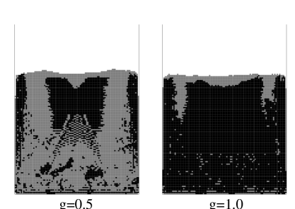
Figure 6: Pattern of loose (grey) and close (black) states for $g=0.5$ (left) and $g=1$.

Figure 6 shows how these loose and close-packed regions are distributed through the pile for the same two values of $g$. The top halves of each pile share similar features: both have a layer of loosely-packed sand on top, where there is no other sand to weigh it down and compress it. Immediately below the surface in the center there is a region of tightly-packed sand, which dips farther below the surface in the center of the pile than to either side. This region is flanked by columns of loosely-packed sand, which are in turn flanked by dense sand up against the edges of the box. The differences in the two piles are mostly at the bottom: the run with less gravity is mostly loose-packed in the bulk of the pile, while the run with more gravity is tighter. Note however that in neither case is the density uniform: one can find patches of both types in both piles. In particular, the patterns in the center of the $g=0.5$ pile may hint at the stress chains that are seen in experiment.

VII Rotating a Sand Pile

VII.1 Set-up

One of the standard ways to probe a granular system is to rotate it about some horizontal axis. This method demonstrates several characteristics of a granular material, and the most important of these is the angle of repose. Actually, there are (at least) two such angles associated with rotation. If one begins with sand in a cylindrical container, having a horizontal free surface, and then begins to rotate the cylinder about its axis, the surface of the sand will increase in slope along with the container’s rotation until it reaches some critical slope, at which point an avalanche will restore the surface to a more horizontal state. This we might call a “static” angle of repose, $\theta_{s}$. If one continues to rotate the cylinder, then one of two things will happen:

1. If the rotation is slow enough, then the flow along the surface will come to a stop before a further increase in slope should cause an avalanche again. The result is a periodic, intermittent flow, and the interface oscillates about some average angle.

2. If the rotation is faster, the flow from the first avalanche does not have time to stop before the next avalanche begins. The system settles into a state where there is a continuous flow along the surface, and the interface maintains a constant angle with the horizontal.

In both cases, we may take the mean angle that the surface makes with the horizontal over time and call it a “dynamic” angle of repose, $\theta_{d}$. In the periodic case, a quantity as important as the angle of repose is the size of the fluctuation about that angle, $\delta_{d}$. The actual values of these angles seems to depend experimentally on a number of factors, including particle size and shape, the humidity of the air, how the pile is formed, boundary conditions, and so forth. The experimental results of Jaeger et al. JLN , for instance, find that spherical glass beads with diameters of about half a millimeter show a dynamic angle of repose of 26^∘, with a fluctuation of 2.6^∘; while rough aluminum-oxide particles with the same diameter show a higher angle, 39^∘, with a fluctuation of 5^∘. These seem to be typical values. What will be most important in our qualitative analysis is that these angles exist and are non-negligible.

We set out to find evidence of these two angles in our model. To better match experiments in this field, we move from a rectangular box to a circular one having a diameter of 100 lattice sites and the same no-slip boundary conditions. We grow a sand pile here as we did before: Figure 7 shows the pattern of loose and close-packed states in a pile formed in our circular container.

Figure 7: Pattern of loose (grey) and close (black) states for $g=1$ in a circular container. It is interesting that this looks more like the lower gravity distribution in the rectangular box, in Figure 6, with a clump of high density floating on top of a low-density sea. This is probably due to the smaller amount of total mass in this system.

To best mimic rotation under experimental conditions, one would ideally set up rotating boundary conditions, giving a constant velocity to the sand at the edge of the container. This has turned out to be difficult to do in practice: one reason is that, due to the lattice, our boundary is not a perfect circle, and there is a tendency for mass to “leak” in or out of the boundaries when the boundary conditions are not strictly no-slip. Because of this, we choose to implement rotation by rotating gravity with a constant period of rotation $T$.

To look for an angle of repose we need to measure the angle that the interface makes with the horizontal (that is, the normal to gravity). The most direct way to do this is to fit the interface of the pile with a line, and measure the angle that this line makes with the horizontal. This is indeed one of our probes: we define as our interface those points which are in the pile ($\rho>0.5$) which have a nearest neighbor outside of the pile, and, to reduce boundary effects, we throw out those points that are not within one half radius from the center.

This method should be ideal, but because of the finite size of our system, this measure ends up depending on only a few points which makes it sensitive to various local perturbations. For this reason, we introduce another measure which we call the “bulk angle” (where the first might be called the “surface angle”). This latter measure is simply the angle that a line passing through the center of the container and the center of mass makes with the vertical. This measure depends on the entire system and so is less sensitive to noise. It will be equal to the surface angle in the event that the pile has reflection symmetry across the vertical axis; it will differ from the surface angle by some fixed amount if the shape of the pile during rotation is asymmetric but constant. Figure 8 shows a plot of the two measures for a typical run.

Figure 8: The behavior of the surface and bulk angles for a typical run ($T=200$). Notice the overall similarity in the shape of the two plots, although the bulk angle has a much smoother curve. The bulk angle is consistently above the surface angle, suggesting that the pile has an asymmetric shape. (All angles are measured in degrees.)

VII.2 Static Angle of Repose

With the surface angle and bulk angle measures in place, let us look systematically at our data. First, we consider the behavior of the pile in the first moments of rotation, with three different periods $T$ (Figure 9).

Figure 9: The behavior of the bulk (left) and surface angles during the first 45^∘ of rotation, for three rotation speeds: $T=200$, $280$, and $400$. The horizontal axis shows the angle through which the container has been rotated.

In all three cases the behavior is similar: as the container turns, the interface’s slope increases, until its angle reaches some maximum and begins to decline due to one or more avalanches. Clearly, there is a static angle of repose here, which depends on the rotation speed. Notice, however, that if there were no activity in the sandpile before the first maximum in the angle, then the curve would follow the straight line denoted in the figure as “solid” until turning downward. Instead, it seems that the surface is losing slope, lagging behind the container, from a very early time: there is some preliminary flow in the pile, even before the first major avalanche.

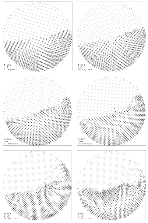
Figure 10: Still frames depicting the momentum flow in our pile in the initial stages of rotation, in gravity’s frame of reference. The darker arrows represent sites in the pile, while the lighter arrows are the very low-density sites above the pile. The length of each arrow is proportional to the momentum, $\rho\vec{v}$, of that particular site. For legibility, each arrow is actually the average of four lattice sites.

Figure 10 contains six snapshots of the flow during this initial period, with $T=200$. All of the pictures here are in the lab frame (that is, gravity’s frame), so the first picture ($t=4$) shows the pile moving in unison with the container, as if it were a solid and fastened to the walls. At $t=8$, however, things are beginning to change: the center of rotation seems to have moved to the right and downward, and the sand coming up on the right side is beginning to curve over to the left. The result of this action is seen in the next picture, where there is a definite flow along the surface of the pile. Notice that, even though there is surface flow, it is not enough to prevent the angle of the interface from climbing, according to Figure 9. The next picture, at $t=16$, shows the surface flow continuing, and also that sand is beginning to climb up the side of the right wall, due to our no-slip boundary conditions. At $t=20$, a major avalanche begins, so that the angle of the interface begins to fall (see Figure 9; this corresponds to 36^∘ on that figure’s horizontal axis). The last picture ($t=30$) shows a much larger flow of material than seen earlier.

In short, there is clearly an initial period where the sand moves with the container and where there is no surface flow, evidence for a nonzero static angle of repose. Recall from section II that this effect is due to the need of the pile to dilate before it can flow. In our model, the close-packed sites are the ones which are restricted in their ability to dilate (because of the barrier in the free energy). Thus, if the pile is dilating during this flow, we expect that the number of close-packed sites in the pile must be decreasing. Figure 11 shows that this is indeed so.

Figure 11: The number of close-packed sites for a cylindrical system rotated at a rate of $T=200$. Plotted against this (and on a different $y$-axis) is the bulk angle of the system, for comparison. Notice that the bulk angle does not stop its ascent until after the number of close-packed sites have begun to decline, and the pile has dilated.

VII.3 Dynamic Angle of Repose

We next consider how the pile behaves under further rotation with three or more turns of the system. Figure 8 above shows the behavior of the bulk and surface angles over three complete revolutions, for $T=200$. Figure 12 below compares the bulk angles between $T=200$ and $T=1600$ over three revolutions.

Figure 12: The bulk angle over three revolutions for two different speeds of rotation. The horizontal axis is again scaled to show the angle through which the container has rotated, rather than the time taken.

Most notable in Figure 12 is that the average slope of the interface is larger for a faster rate of rotation. Also, the slower system deviates much less from a constant angle than does the faster one, with more jaggedness suggesting frequent small avalanches. These points suggest an inertial effect: in the faster case the sand does not have as much time to avalanche and level its interface, while the slower case has a number of short avalanches that help to keep its interface closer to the horizontal. However, the slow line is occasionally punctuated by large avalanches that dip into the negative: curiously, the interface seems to tilt in the direction opposite that of rotation every once in a while. Figure 13 looks at one of these dips more closely. Apparently, even with the constant small avalanches that we see in the bulk angle in the slowly rotating case, there is still a build-up of potential energy that must be released by these larger events.

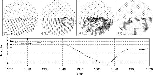
Figure 13: An instance in the slow ($T=1600$) rotation of the pile where the bulk angle dips below zero. The four flow diagrams show the momentum of the pile at $t=1320$, $1340$, $1360$, and $1380$. The mechanism by which the angle drops is a large vortex in the pile which give individual grains a large momentum to the left. Notice how calm the pile is before and after this event: certainly this is intermittent behavior.

All of our tests so far show a nonzero dynamic angle of repose, but to rule out the possibility that these angles are due to viscosity or inertia, it is best to find how the average angle (bulk or surface) depends on the period of rotation $T$, and from this relationship extrapolate to $T\to\infty$. With this in mind we measure the average bulk and surface angles over time for several rotation speeds, and, in Figure 14, plot them versus the rotation speed $1/T$.

Figure 14: The average surface (left) and bulk angles are the center points in each column of their respective plots; the outer points delineate one standard deviation above and below. Each data point represents one run of the system, consisting of the last two of three complete revolutions; the first turn was thrown out to diminish initial effects. The lines are power law fits.

The first thing to note in these plots is that neither angle is going to zero in the limit of small angular velocities: there is a definite non-zero angle of repose in our system. This angle, about 2.5^∘, is quite small compared to experiment where typically one finds angles of repose on the order of 30^∘JLN ; Rajchenbach .

Table 1: We fit the angles of repose in figure 14 to the model $\theta=\theta_{0}+cT^{\alpha}$.

	$c$		$\alpha$		$\theta_{0}$		$\chi^{2}$
bulk angle	10700$\pm$	4100	-1.35$\pm$	0.07	2.49$\pm$	0.15	0.148
surface angle	83.7$\pm$	105.0	-0.555$\pm$	0.275	2.51$\pm$	1.12	0.780

It is interesting to fit the angles in Figure 14 to a power law

$$\theta=\theta_{0}+cT^{\alpha}.$$ (26)

Such fits are shown in the figure, with the parameters given in Table 1. The intercepts $\theta_{0}$ are positive, confirming a non-zero angle of repose. The fit to the surface angle is not quantitative, but for the average bulk angle the power law fits well, with an exponent of $-1.4$.

These data points come from single runs, and averaging over an ensemble of initial conditions may make the fits more quantitative.

Experimentally, Rajchenbach Rajchenbach finds that the angular velocity $\Omega$ goes as

$$\Omega\sim(\theta-\theta_{d})^{m}$$ (27)

where $m=0.5\pm 0.1$. This corresponds to

$$\theta\sim T^{-2\pm 0.4}$$ (28)

Of our two measures, the bulk angle comes closer to matching experiment, but there is still some discrepancy that needs to be addressed.

Finally, to compare the surface and bulk angles with each other. For high-speed rotations, the bulk angle is higher on average than the surface angle, reflecting the plume of material that creeps up the side of the container (which is accounted for in a bulk calculation, but specifically excluded from the surface angle). The surface angle actually seems to level off at high speeds. At lower speeds, the bulk angle actually dips below the surface angle, suggesting that the plume has disappeared (as is seen in Figure 13). Notice that the fluctuations in the surface angle are larger than those in the bulk angle (the former depending on fewer lattice sites and thus more volatile), and that in both angles these fluctuations get smaller as one reduces the speed of rotation (but do not seem to go to zero).

VIII Discussion

We present evidence that one can create a nonlinear hydrodynamical model for granular materials that depends only on density and momentum fields. Qualitatively, our model demonstrates many key features of sand, including a sharp interface, a relatively uniform density, a nonzero angle of repose, and a metastable structure. The method allows us to follow the pile from creation forward, in static and dynamic situations, and the model generally behaves like a sand pile.

There are several ways in which the model could be improved. The angles of repose seen here are too small when compared to experiment, and the way that the angles scale with rotation speed is at odds with Rajchenbach’s findings. This may not be a problem since we have not yet looked at the variation of the angle of repose with the parameters characterizing the model. An explanation for the difference may also lie in the fact that our rotation probe differs from the typical experimental method of rotating a sandpile. In our simulations, where we rotate gravity, every particle feels the external force directly and immediately. In experiment, where the container is rotated, the external force must be transmitted inward from the boundaries. This difference may be enough to account for the discrepancy between simulational and experimental outcomes. One may be able to mimic the rotation of the container in our model by introducing centrifugal forces into the system. Such forces would have a magnitude of

$$F_{c}=\rho r\left(2\pi\over T\right)^{2},$$

where $r$ is the distance from the center of the container. Our round container has a diameter of 100 units, so $r\leq 50$, while $\rho\sim 1$ and the fastest rotation speed we use is $T=200$; thus these centrifugal forces would have a magnitude of $0.05$, which is small (though not negligible) compared to the main acting force of gravity, which is of magnitude roughly equal to $1$. Thus centrifugal forces may provide some quantitative effect, but in our initial, qualitative presentation here we deemed it unnecessary to include them.

Another way of improving the model is to remove the constraint that the loose-packed regions have a single fixed density. There are many non-optimal, metastable ways to pack particles together, having a range of different densities. One solution may be to allow the position of the loose-packed well to fluctuate slightly at random through the pile. There are several plausible ways of implementing this idea, which we intend to pursue.

We have only begun to extract information using our model; there are other probes we can use to perturb our system. Shaking can cause the pile to slowly settle into a denser state; we hope to find the logarithmic time dependence seen in compactification experiments Knight . Applying pressure to the system may allow us to investigate force propagation in the pile, and determine the nature of stress chains. It should be possible to modify the model to depict a pile made up of two or more types of particles, to investigate the phenomena of unmixing and the Brazil nut effect in a hydrodynamical setting. The flexibility of the fluctuating nonlinear hydrodynamical approach gives us a wide range of avenues to investigate.

Appendix: Specification of the Free Energy Density

The first potential in Figure 1 is made up of four terms:

$$f_{a}(\rho)=f_{\text{clump}}(\rho)+f_{\text{large}}(\rho)+f_{\text{negative}}(\rho)+f_{\text{entropy}}(\rho)$$ (29)

where

$$f_{\text{clump}} = -\frac{1}{2}u_{0}\rho^{2}$$ (30)

$$f_{\text{large}} = Be^{\lambda(\rho^{2}-1)}$$ (31)

$$f_{\text{negative}} = U_{1}e^{-\lambda_{1}\rho}.$$ (32)

The first term models the clumping behavior of sand mentioned in property 1 in section II. The second term models the ultimate incompressibility of the sand grains: $B$ is chosen so that the minimum of the well is at $\rho=1$. The third term prevents the densities from becoming negative by putting a barrier at zero density.

We have not given the definition for $f_{\text{entropy}}$ yet. Our original intent was to have this term model the behavior of the very dilute gas that exists above our sand pile. So that the low-density regions show a Boltzmann distribution, we used the standard gas entropy term

$$f^{\prime}_{\text{entropy}}=A(\rho\ln(\rho/\rho_{0})-\rho)$$ (33)

with $\rho_{0}=0.05$. However, this was a source of numerical instability, and since our focus was the pile and the high-density regions, we replaced this with a simpler term,

$$f_{\text{entropy}}=A\rho.$$ (34)

The reason we did not eliminate the term entirely was that the original term created a shallow minimum around $\rho=0.05$, and for consistency we decided to keep that minimum there which the linear term allows us to do.

Clearly, this model has a lot of parameters, and one part of our future work will be to find optimal values for these parameters. Our current choices were selected because they gave realistic results: we set $u_{0}=2$, $\lambda=40$, $U_{1}=0.6$, $\lambda_{1}=400$, and $A=0.2$. To satisfy the requirement that the minimum of the potential be at $\rho=1$, we set $B=\frac{1}{2\lambda}(u_{0}-A)$.

The barrier introduced in Figure 1b is described by

$$f_{\text{barrier}}=u_{b}e^{-{1\over 2}k(\rho-\rho_{b})^{2}},$$ (35)

where $u_{b}=1.5$, $\rho_{b}=0.99$, and $k=10^{5}$. The two wells in the final potential are described by

$$f_{\text{well${}_{n}$}}=-u_{n}e^{-{1\over 2}k(\rho-\rho_{n})^{2}},$$ (36)

where $\rho_{1}=0.98$ and $\rho_{2}=1.01$, $u_{1}=0.25$ and $u_{2}=0.4$, and $k$ is the same as in the expression for the barrier.

- (1) H. M. Jaeger, S. R. Nagel, and R. P. Behringer, Rev. Mod. Phys. 68, 1259 (1996).
- (2) Nonlinear hydrodynamics has been successful in treating nonlinear phenomena in a wide variety of physical systems ranging from magnets lanlif to superfluids foot-superfluids . The method has been particularly useful in treating nonlinear behavior like critical phenomena Ma , nucleation theory Langer , and unstable growth Bray . It should be appreciated that nonlinear hydrodynamics is a more complete theory than long wavelength linearized hydrodynamics. Conventional hydrodynamics Martin , expressed in terms of observable transport coefficients and such, emerges from NH as a limiting regime.
- (3) A. P. Malozemoff and J. C. Slonczewski. Magnetic Domain Walls in Bubble Materials. Academic Press, New York (1979).
- (4) The time-dependent Ginzburg-Landau equation has played a central role in treating the dynamic properties of superfluids and superconductors.
- (5) J. S. Langer and L. Turski, Phys. Rev. A 8, 3230 (1973).
- (6) A. J. Bray, Adv. Phys. 43, 357 (1994).
- (7) P. C. Martin, O. Parodi, and P. S. Pershan, Phys. Rev. A 6, 2401 (1972).
- (8) S. McNamara and W. R. Young, Phys. Fluids A 4, 496 (1992); Phys. Rev. E 53, 5089 (1996); Y. Du, H. Li, and L. P. Kadanoff, Phys. Rev. Lett. 74, 1268 (1995); E. L. Grossman, T. Zhou, and E. Ben-Naim, Phys. Rev. E 55, 4200 (1997); E. L. Grossman, Phys. Rev. E 56, 3290 (1997).
- (9) C. H. Liu et al., Science 269, 513 (1995); D. M. Mueth, H. M. Jaeger, and S. R. Nagel, Phys. Rev. E 57, 3164 (1998).
- (10) J. B. Knight, C. G. Fandrich, C. N. Lau, H. M. Jaeger, and S. R. Nagel, Phys. Rev. E 51, 3957 (1995) and subsequent papers.
- (11) P. Evesque and J. Rajchenbach, Phys. Rev. Lett. 62, 44 (1989); E. Clement, J. Duran, and J. Rajchenbach, Phys. Rev. Lett. 69, 1189 (1992); T. H. Metcalf, J. B. Knight, and H. M. Jaeger, Physica A 236, 202 (1997); 70, 3728 (1993); F. Melo, P. Umbanhower, and H. L. Swinney, Phys. Rev. Lett. 72, 172 (1994).
- (12) J. Lee, J. Phys. A 27, 257 (1994); M. Bourzutschky and J. Miller, Phys. Rev. Lett. 74, 2216 (1995); H. Hayakawa, S. Yue, and D. C. Hong, Phys. Rev. Lett. 75, 2328 (1995); H. Hayakawa and D. C. Hong, Phys. Rev. Lett. 78, 2764 (1997); H. Hayakawa and D. C. Hong, Two Hydrodynamic Models of Granular Convection, arXiv:cond-mat/9703086.
- (13) S. Ogawa, in Proceedings U.S.-Japan Seminar on Continuum-Mechanical and Statistical Approaches in the Mechanics of Granular Materials, edited by S. C. Cowin and M. Satake. Gakujutsu Bunker Fukyukai, Tokyo, Japan (1978); S. B. Savage and D. J. Jeffrey, J. Fluid Mech. 110, 255 (1981); J. T. Jenkins and S. B. Savage, J. Fluid Mech. 130, 186 (1983); P. K. Haff, J. Fluid Mech. 134, 401 (1983); P. K. Haff, J. Rheol. 30, 931 (1986); C. K. K. Lun and S. B. Savage, J. of App. Mech. 54, 47 (1987); C. S. Campbell, Annu. Rev. Fluid Mech. 22, 57 (1990); Y. M. Bashir and J. D. Goddard, 35, 849 (1991); X. Zhuang, A. K. Didwania, and J. D. Goddard, J. Comput. Phys. 121, 331 (1995).
- (14) If one uses kinetic theory, one has the involved intermediate stage in the theory of deriving hydrodynamics equations from which one extracts observables.
- (15) I. Goldhirsch and G. Zanetti, Phys. Rev. Lett. 70, 1619 (1993)
- (16) O. Reynolds, Philos. Mag. 20, 469 (1885).
- (17) A. Rosato, K. J. Strandburg, F. Prinz, and R. H. Swendsen, Phys. Rev. Lett. 58, 1038 (1987).
- (18) S. Ma and G. F. Mazenko, Phys. Rev. B 11, 4077 (1975) show how a broad class of models can be applied to dynamic critical phenomena.
- (19) S. P. Das and G. F. Mazenko, Phys. Rev. A 34, 2265 (1986).
- (20) This form is the simplest we can assume, and there are a series of more sophisticated choices one can investigate.
- (21) Actually, we use for computational reasons. When no row has exactly this average density, which is often the case, interpolation is used.
- (22) H. M. Jaeger, C. H. Liu, and S. R. Nagel, Phys. Rev. Lett. 62, 40 (1989).
- (23) J. Rajchenbach, Phys. Rev. Lett. 65, 2221 (1990).