Fate of Zero-Temperature Ising Ferromagnets

Abstract

We investigate the relaxation of homogeneous Ising ferromagnets on finite lattices with zero-temperature spin-flip dynamics. On the square lattice, a frozen two-stripe state is apparently reached approximately 1/4 of the time, while the ground state is reached otherwise. The asymptotic relaxation is characterized by two distinct time scales, with the longer stemming from the influence of a long-lived diagonal stripe “defect”. In greater than two dimensions, the probability to reach the ground state rapidly vanishes as the size increases and the system typically ends up wandering forever within an iso-energy set of stochastically “blinking” metastable states.

PACS Numbers: 64.60.My, 05.40.-a, 05.50.+q, 75.40.Gb

What happens when an Ising ferromagnet, with spins endowed with Glauber dynamics[1], is suddenly cooled from high temperature to zero temperature ($T=0$)? A first expectation is that the system should coarsen[2] and eventually reach the ground state. However, even the simple Ising ferromagnet admits a large number of metastable states with respect to Glauber spin-flip dynamics. Therefore at zero temperature the system could get stuck forever in one of these states.

In this Letter, we present evidence that the behavior of such a kinetic Ising model is richer than either of these scenarios. While the ground state is always reached in one dimension, there appears to be a non-zero probability that the square lattice system freezes into a “stripe” phase, at least for equal initial concentrations of $\uparrow$ and $\downarrow$ spins[3]. The relaxation is governed by two distinct time scales, the larger of which stems from a long-lived diagonal stripe “defect”. On hypercubic lattices ($d\geq 3$), the probability to reach the ground state vanishes in the thermodynamic limit and the system ends up wandering forever on an iso-energy subset of connected metastable states. Again, the relaxation seems to be characterized by at least two time scales. It bears emphasizing that these long-time anomalies require that the limit $T\to 0$ is taken before the thermodynamic limit $L\to\infty$; very different behavior occurs if $L\to\infty$ before $T\to 0$[4].

We can easily appreciate the peculiarities of zero-temperature dynamics for odd-coordinated lattices, such as the honeycomb lattice. Here any connected cluster in which each spin has at least 2 aligned neighbors is energetically stable in a sea of opposite spins. For any initial state, a sufficiently large system will have many such stable defects. Because the number of such metastable states generally scales exponentially with the total number of spins $N$, the system necessarily freezes into one of these states. However, on even-coordinated lattices the number of metastable states grows as a slower, stretched exponential function of $N$, and they affect the asymptotic relaxation in much more subtle way.

We therefore study the homogeneous Ising model, with Hamiltonian ${\cal H}=-J\sum_{\langle ij\rangle}\sigma_{i}\sigma_{j}$, where $\sigma_{i}=\pm 1$ and the sum is over all nearest-neighbor pairs of sites $\langle ij\rangle$. We assume initially uncorrelated spins, with $\sigma_{j}(t=0)=\pm 1$ equiprobably, which evolve by zero-temperature Glauber dynamics[1], corresponding to a quench from $T=\infty$ to $T=0$. We focus on $d$-dimensional hypercubic lattices with linear size $L$ and periodic boundary conditions. Most of our results continue to hold for free boundary conditions and on arbitrary even-coordinated lattices.

Glauber dynamics at zero temperature involves picking a spin at random and considering the energy change $\Delta E$ if the spin were flipped. If $\Delta E<0$ ($>$0), the flip is accepted (rejected), while if $\Delta E=0$, the attempt is accepted with probability 1/2. After each event, time is updated by $1/L^{d}$, so that each spin undergoes, on average, one update attempt in a single time unit. In practice, we update only the flippable spins (those with $\Delta E\leq 0$) and update the time by $1/({\rm number\ of\ flippable\ spins})$. For each initial state, one realization of the dynamics is run until the final state. At $T=0$, metastable states in this dynamics have an infinite lifetime and these can prevent the equilibrium ground state from being reached. This is the basic reason why dynamics at $T=0$ is very different from that of small positive temperature.

In one dimension, it is easy to determine the ultimate fate of the system[5]. In $T=0$ Glauber kinetics, the expectation value of the $i^{\rm th}$ spin, $s_{i}\equiv\langle\sigma_{i}\rangle$, obeys the diffusion equation and therefore the average magnetization $\langle m\rangle={1\over L}\sum_{j}s_{j}$ is conserved[1]. Since there are no metastable states in one dimension, the only possible final states are all spins up or all spins down. For initial magnetization $m(0)$, a final magnetization $m(\infty)=m(0)$ can be achieved only if a fraction ${1\over 2}(1+m(0))$ of all realizations of the dynamics ends with all spins up and a fraction ${1\over 2}(1-m(0))$ with all spins down.

On the square lattice, there exists a huge number of metastable states which consist of alternating vertical (or horizontal) stripes whose widths are all $\geq 2$. These arise because in zero-temperature Glauber dynamics a straight boundary between up and down phases is stable; a reversal of any spin along the boundary increases its length and raises the energy. Note that a stripe of width one is not stable because it can be cut in two at no energy cost by flipping one of the spins in the stripe.

FIG. 1.: Probability that an $L\times L$ square eventually reaches a stripe state as a function of $1/\log_{2}L$ for $L$ up to 1024. Each data point (with error bars) is based on $10^{5}$ initial spin configurations for $L\leq 256$, and then 13,500 and 2,700 configurations respectively for $L=512$ and $L=1024$.

The mere existence of these metastable states implies that a finite sample may not reach the ground state. However, one might expect that the probability to reach the ground state approaches unity as the system size grows: $\lim_{L\to\infty}P_{\rm gs}=1$. Our numerical simulations on $L\times L$ squares appear to disagree with this expectation (Fig. 1). The probability $P_{\rm gs}$ grows extremely slowly with $L$ and extrapolates to a value of approximately $3/4$ as $L\to\infty$, so that the probability to reach a two-stripe state, $P_{\rm str}=1-P_{\rm gs}$ would be non-zero. We also find that states with more than two stripes almost never appear.

FIG. 2.: Final magnetization distribution on the (a) square, and (b) cubic lattices. On the square lattice, this distribution narrows as $L$ increases, but appears to reach a non-singular limit. On the cubic lattice, data collapse occurs even at small sizes. The number of realizations is $10^{5}$ for the square and $\geq 10^{4}$ for the cubic lattices.

When the two-stripe state is reached on the square lattice, both stripes have width typically of the order of $L/2$, as seen by a gradual narrowing of the continuous component $C_{\rm 2d}(m)$ of the final magnetization distribution, $F_{2d}(m)={1\over 2}P_{\rm gs}\left[\delta(m-1)+\delta(m+1)\right]+P_{\rm str}C_{2d}(m)$ (Fig. 2(a)). However, as $L$ increases the magnetization distribution appears to converge to a finite-width scaling limit. On the simple cubic lattice, there are many more metastable state topologies and also relatively more states with narrow stripes, so that there is a larger probability that the final magnetization is close to $\pm 1$. The final magnetization distribution also exhibits good data collapse even at relatively small system sizes. Strikingly, the final magnetization distribution on the cubic lattice is well fit by $F_{3d}(m)={3\over 4}(1-m^{2})$ (Fig. 2(b)).

Intriguing behavior is also exhibited by the survival probability $S(t)$ that the system has not yet reached its final state by time $t$. As shown in Fig. 3, $S(t)$ is controlled by two different time scales. On a semi-logarithmic plot, $S(t)$ lies on one straight line with large negative slope for intermediate times and crosses over to another line with smaller negative slope at long times. In this intermediate time regime, the energy decays as $t^{-1/2}$, as expected[2] The crossover in $S(t)$ occurs when domains, which grow according to the classical $t^{1/2}$ law[2], reach the system size. This gives the crossover time $\tau_{c}\propto L^{2}$.

Quite surprisingly, the source of the long-time anomaly in $S(t)$ arises from the approximately 4% of the configurations in which a diagonal stripe appears (Fig. 4). On the torus, this configuration consists of one stripe of $\uparrow$ spins and another of $\downarrow$ spins which, by symmetry, have width of order $L$. Each of these stripes winds once in both toroidally and poloidally on the torus; they cannot evolve into straight stripes by a continuous deformation of the boundaries. Consequently a diagonal stripe configuration should ultimately reach the ground state.

FIG. 3.: Time dependence of the survival probability $S(t)$ on $L\times L$ squares. Main graph: $S(t)$ versus $t/M_{10}$ to highlight the long-time exponential tail, where $M_{k}\equiv\langle t^{k}\rangle^{1/k}$ is the $k^{\rm th}$ reduced moment of the time to reach the final state. Scaling sets in after $S(t)$ has decayed to approximately 0.04. Inset: $S(t)$ versus $t/M_{1/10}$ to highlight the scaling and the faster exponential decay in the intermediate-time regime.

Diagonal stripes are also extremely long-lived. For $L=200$, for example, the time for such a configuration to reach the final state is two orders of magnitude larger than the typical time. To understand this long lifetime, we view a diagonal boundary as an evolving interface in a reference frame rotated by $45^{\circ}$[6].

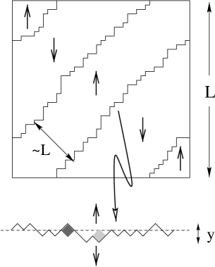
FIG. 4.: Diagonal stripe configuration on the square lattice. The lower portion shows part of one interface rotated by $45^{\circ}$. Zero-temperature Glauber dynamics allows for either particle deposition at the bottom of a valley (light-shaded square) – corresponding to the spin-flip even $\uparrow\to\downarrow$ – or particle evaporation from a peak (filled square) – corresponding to $\downarrow\to\uparrow$.

In this frame (Fig. 4 lower), a spin flip is equivalent to a “particle” which either deposits at the bottom of a valley ($\uparrow\to\downarrow$) or evaporates from a peak ($\downarrow\to\uparrow$). In a single time step each such event occurs with probability 1/2. For an interface with transverse dimension of order $L$, let us assume that there are of the order of $L^{\mu}$ such height extrema. Ref. [6] predicts $\mu=1$, but we temporarily keep the value arbitrary for clarity. Accordingly, in a single time step, where all interface update attempts occur once on average, the interface center-of-mass moves a distance $\Delta y\sim L^{\mu/2}/L$. This gives an interface diffusivity $D\sim(\Delta y)^{2}\sim L^{\mu-2}$. We then estimate the lifetime $\tau_{\rm diag}$ of a diagonal stripe as the time for the interface to move a distance of order $L$ to meet another interface. This gives $\tau_{\rm diag}\sim L^{2}/D\sim L^{4-\mu}$. Using the results of Ref. [6], we expect $\tau_{\rm diag}\propto L^{3}$.

The survival probability reflects these two time scales (Fig. 3), and their $L$ dependence is cleanly visible in the reduced moments $M_{k}\equiv\langle t^{k}\rangle^{1/k}$ of the time until the final state is reached. The main contribution to the moments with $k<1$ comes from short-lived configurations, while for $k>1$ the main contribution comes from long-lived diagonal-stripe configurations. Our data for $M_{k}$ with $k<1$ scales approximately as $L^{2}$, while for $k>1$, $M_{k}$ scales roughly as $L^{3.5}$, somewhat faster growth than expected (Fig. 5).

In greater than two dimensions, the probability to reach the ground state rapidly vanishes as the system size increases. For example, $P_{\rm gs}\approx 0.04$ and $0.003$ for cubic lattices of linear dimension $L=10$ and 20. For larger lattices, the ground state has not been reached in any of our simulations. One obvious reason why the system “misses” the ground state is the rapid increase in the number of metastable states with spatial dimension. This proliferation of metastable states makes it more likely that a typical configuration will eventually reach one of these states rather than the ground state. Another striking feature is that many metastable states in three dimensions form connected iso-energy sets, while metastable states are all isolated in two dimensions. Thus a three-dimensional system can end up wandering forever on one of these connected sets.

FIG. 5.: Dependence of $M_{k}\equiv\langle t^{k}\rangle^{1/k}$ on $L$. Shown are the cases $k=1$ (dashed curve), $k=1/2$ ($\Box$), 1/4 ($\Delta$), and 1/10 ($\circ$), as well as $k=2$, 4, and 10 (corresponding filled symbols). The thin straight lines have slopes 2 and 3.5.

A specific example from a simulation on a small cube is sketched in Fig. 6. By viewing the spins as cubic blocks, the cluster of aligned spins appears as a “building” with a $2$-storey section (marked 2), an adjacent $3$-storey section, and a section (marked $\infty$) which wraps around the torus in the vertical direction and rejoins the building on the ground floor. The wiggly lines indicate that building sections also wrap around in the $x$- and $y$-directions.

FIG. 6.: A stochastic blinker on the cubic lattice.

The sites marked by $\times$ are “blinkers”. Consider the leftmost such site. Since there are three directions where the nearest neighbors are part of the building, this leftmost spin can flip with zero energy cost. If this occurs, then its right neighbor, which was initially stable, can now flip with no energy cost. This sequence can continue until the right edge of the $\infty$ section of the building but no further. Therefore this third-storey addition performs a random walk, constrained to move forever in the interval marked by the $\times$ sites. While this construction appears idiosyncratic, such a structure is the basic element of generic blinkers on even-coordinated Cayley trees.

Another feature of the final state is that it almost always consists of only two interpenetrating clusters which both percolate in all three Cartesian directions. These two percolating clusters must each contain no convex corners to be stable at $T=0$. While there are also metastable states with many components and metastable states with components percolating in one or in two directions, such configurations are generally not reached when the system is large enough.

The energy decay on the cubic lattice also suggests that there exists more than one relaxational time scale. Initially, the energy decreases systematically in a manner consistent with a power-law decay. At longer times, however, the energy exhibits plateaux of increasing duration, punctuated by small energy decreases. Ultimately the final energy is reached, after which constant-energy stochastic blinking occurs ad infinitum. Our data for the time until the appearance of the first energy plateau scales roughly as $L^{3}$, while the time to reach the final energy seems to increase faster than any power of $L$.

The phase-space structure of the metastable states appears to be a crucial element in understanding the fate of Ising ferromagnets. The simplest aspect is to estimate the number of metastable states $M_{d}(N)$ as a function of the spatial dimension $d$ and number of spins $N=L^{d}$. In two dimensions, a metastable state contains alternating horizontal or vertical stripes of up and down spins, with each stripe of width $\geq 2$. This is identical to the number of ground states of a periodic Ising chain with nearest-neighbor ferromagnetic interaction $J_{1}$ and second-neighbor antiferromagnetic interaction $J_{2}$ (axial next-nearest neighbor Ising (ANNNI) model), when $J_{2}=-J_{1}/2$. For the chain with open boundaries, the number of metastable state was previously found in terms of the Fibonacci numbers[7]. For the periodic system the number of metastable states is

$$M_{2}={g^{L-1}-(-g)^{-L+1}\over\sqrt{5}}-{2\over\sqrt{3}}\,\sin{\pi\over 3}(L-1)+2,$$ (1)

where $g={1\over 2}(1+\sqrt{5})$ is the golden ratio, and the first term is just the ANNNI model degeneracy. Eq. (1) therefore gives $M_{2}(V)\sim e^{A_{2}\sqrt{N}}$ with $A_{2}=\ln g$.

For $d=3$, we give a lower bound for the number of metastable states by generalizing the stripe states of the square lattice. Consider states which consist of an array of straight filaments such that each filament cross-section is rectangular and the “Manhattan” distance between any two rectangles is $\geq 2$. The number of packings of such filaments is of the order of $\exp(cL^{2})$, where $c$ is a constant. This gives the lower bound for the number of metastable states, $M_{3}(N)>\exp(cN^{2/3})$. This same construction in $d$ dimensions gives $M_{d}(N)>\exp(cN^{(d-1)/d})$. While we have not succeeded in constructing an upper bound, it seems plausible that this bound has the same functional form as the lower bound; hence $M_{d}(N)\sim\exp\left(A_{d}N^{(d-1)/d}\right)$. In addition, it can be verified that the number of metastable states on the Cayley tree grows exponentially with the number of spins. Thus metastable states become relatively more numerous as the dimension increases and their influence on long-time kinetics should correspondingly increase.

In summary, the homogeneous Ising ferromagnet exhibits surprisingly rich behavior following a quench from infinite to zero temperature. On the square lattice, there appears to be a non-zero probability of reaching a static two-stripe state. Evolution via a diagonal stripe configuration is responsible for a two-time-scale relaxation kinetics. On the cubic lattice, the probability of reaching both the ground state or a frozen metastable state vanishes rapidly as the system size increases. The system instead reaches a finite iso-energy attractor of metastable states upon which it wanders stochastically forever.

We thank C. Godrèche, M. Grant, J. Krug, T. Liggett, C. Newman, Z. Rácz, J. Sethna, and D. Stein for helpful discussions, and NSF grant DMR9978902 for financial support.

REFERENCES

- [1] R. J. Glauber, J. Math. Phys. 4, 294 (1963).
- [2] J. D. Gunton, M. San Miguel, and P. S. Sahni in: Phase Transitions and Critical Phenomena, Vol. 8, eds. C. Domb and J. L. Lebowitz (Academic, NY 1983); A. J. Bray, Adv. Phys. 43, 357 (1994).
- [3] Anomalies associated with stripes and other metastable states have been hinted at previously. See e. g., J. Kurchan and L. Laloux, J. Phys. A 29, 1929 (1996); D. S. Fisher, Physica D 102, 204 (1997).
- [4] C. M. Newman and D. L. Stein, Phys. Rev. Lett. 82, 3944 (1999); Physica A 279, 159 (2000).
- [5] See e. g., T. M. Liggett, Interacting Particle Systems, (Springer-Verlag, New York, 1985).
- [6] M. Plischke, Z. Rácz, and D. Liu, Phys. Rev. B 35, 3485 (1987).
- [7] S. Redner, J. Stat. Phys. 25, 15 (1981).