Introduction to the Bethe Ansatz III

Abstract

Having introduced the magnon in part I and the spinon in part II as the relevant quasi-particles for the interpretation of the spectrum of low-lying excitations in the one-dimensional (1D) s=1/2 Heisenberg ferromagnet and antiferromagnet, respectively, we now study the low-lying excitations of the Heisenberg antiferromagnet in a magnetic field and interpret these collective states as composites of quasi-particles from a different species . We employ the Bethe ansatz to calculate matrix elements and show how the results of such a calculation can be used to predict lineshapes for neutron scattering experiments on quasi-1D antiferromagnetic compounds. The paper is designed as a tutorial for beginning graduate students. It includes 11 problems for further study.

I Introduction

In most areas of condensed-matter research, a few model systems outshine all others by their prototypical significance, which promises to encapsulate the essence of a physical phenomenon with little interference of collateral degrees of freedom. In cooperative magnetism, the Ising model, the Heisenberg model, and the Hubbard model, for example, are theoretical many-body systems that have kept generations of researchers fascinated.

The prominence of such models and the abundance of theoretical predictions for many of their physical properties have at times led to a reversal of the traditional relationship between theory and experiment. Instead of theorists proposing and solving models for the purpose of explaining measurements performed on specific materials, we see magneto-chemists and condensed-matter experimentalists at work searching for materials which are physical realizations of the prototypical models.

The focus here is on the one-dimensional (1D) $s=\frac{1}{2}$ Heisenberg antiferromagnet in a magnetic field. The Hamiltonian for a cyclic chain with $N$ sites reads

$$H=\sum_{n=1}^{N}\left[J{\bf S}_{n}\cdot{\bf S}_{n+1}-hS_{n}^{z}\right].$$ (1)

This model is amenable to exact analysis via Bethe ansatz and displays dynamical properties of intriguing complexity. The magnetic field $h$ is a continuous parameter which has a strong impact on most physical properties and which is directly controllable in experiments. The high degrees of computational and experimental control is what makes this system so attractive to researchers.

Physical realizations of Heisenberg antiferromagnetic chains have been known for many years in the form of 3D crystalline compounds with quasi-1D exchange coupling between magnetic ions. The desired properties of the best candidate material include the following: The coupling of the effective electron spins must be highly isotropic in spin space and overwhelmingly predominant between nearest-neighbor magnetic ions along one crystallographic axis. The intra-chain coupling must not be too weak or else it will be hard to study the low-temperature properties, which are of particular interest. It must not be too strong either or else it will be hard to reach a magnetic field that makes the Zeeman energy $hS_{n}^{z}$ comparable to the exchange energy $J{\bf S}_{n}\cdot{\bf S}_{n+1}$.

One compound that fits the bill particularly well is copper pyrazine dinitrate [Cu(C₄H₄N₂)(NO₃)₂], a material that was only recently synthesized in single crystals of sizes and shapes suitable for magnetic inelastic neutron scattering.HSR+99 The most detailed dynamical experimental results to date were made on KCuF₃,NTC+91 in which the intra-chain coupling is considerably stronger, which makes it easier to study low-temperature effects but harder to study magnetic-field effects.

What happens in a magnetic neutron scattering experiment? A beam of monochromatic neutrons, ideally a plane wave with well defined momentum and energy, is scattered inelastically off an array of spin chains via magnetic dipolar interaction between the exchange coupled electron spins and the neutron spin into a superposition of waves with a range of momenta and energies. Each inelastic scattering event causes a transition between two eigenstates of the spin chain. The difference in energy and wave number of the two eigenstates involved must be matched by the energy and momentum transfer of the scattered neutron.

If the measurement is performed at very low temperature, it is reasonable to assume that the observable scattering events predominantly involve transitions from the ground state $|G\rangle$ to excitations $|\lambda\rangle$ with energies and wave numbers within a window preset by the experimental setup. The experiment thus enables us to have a direct look at the excitation spectrum of the spin chain. It probes the spin fluctuations as described by the fluctuation operator

$$S_{q}^{\mu}=N^{-1/2}\sum_{n=1}^{N}e^{iqn}S_{n}^{\mu},\quad\mu=x,y,z$$ (2)

for wave numbers $q=2\pi l/N,l=1,\ldots,N$. Under idealized circumstances, the inelastic neutron scattering cross section is proportional to the dynamic spin structure factor at zero temperature:BL89 ; Furr00

$$S_{\mu\mu}(q,\omega)=2\pi\sum_{\lambda}|\langle G|S_{q}^{\mu}|\lambda\rangle|^{2}\delta\left(\omega-\omega_{\lambda}\right).$$ (3)

Each scattering event with energy transfer $\hbar\omega_{\lambda}\equiv E_{\lambda}-E_{G}$ and momentum transfer $\hbar q\equiv\hbar(k_{\lambda}-k_{G})$ along the chain induces a transition from $|G\rangle$ to $|\lambda\rangle$ and contributes a spectral line of intensity $2\pi|\langle G|S_{q}^{\mu}|\lambda\rangle|^{2}$ to $S_{\mu\mu}(q,\omega)$. For a macroscopic system, the spectral lines are arranged in a variety of patterns in $(q,\omega)$-space, including branches, continua, and more complicated structures. The functions $S_{\mu\mu}(q,\omega)$ thus provide a palette of information about the $T=0$ dynamics of the spin chain.

Unlike in a classical dynamical system, where all motion grinds to a halt at $T=0$, the quantum wheels keep turning – a phenomenon known as zero point motion. For the Heisenberg model (1) in the ground state $|G\rangle$, the quantum fluctuations of any observable ${\cal O}$ of interest can be described by a time-dependent correlation function of the form

$$\langle{\cal O}(t){\cal O}^{\dagger}\rangle\equiv\langle G|e^{iHt/\hbar}{\cal O}e^{-iHt/\hbar}{\cal O}^{\dagger}|G\rangle.$$ (4)

If ${\cal O}$ is conserved ($[{\cal O},H]=0$), then $\langle{\cal O}(t){\cal O}^{\dagger}\rangle=\langle G|{\cal O}{\cal O}^{\dagger}|G\rangle$ is a constant. Different dynamical variables ${\cal O}$ yield different correlation functions for the same ground state $|G\rangle$. The dynamical variable seen by neutrons during the magnetic scattering is $S_{q}^{\mu}$. Fourier transforming (4) with ${\cal O}=S_{q}^{\mu}$ yields the dynamic spin structure factor (3) (Problem 1).

Light scattering, electron scattering, photoemission, and nuclear magnetic resonance are some other experimental techniques used to investigate the dynamics of (1). Different measuring techniques view the same excitation spectrum through lenses of different color, i.e. by transition rates specific to particular fluctuation operators. Hence each experimental probe filters out a specific aspect of the zero point motion by viewing a particular dynamical variable of one and the same system.

The goal set for this column is to teach the reader how to make detailed predictions based on the Bethe ansatz solution of (1) for the inelastic neutron scattering cross section as can be measured on quasi-1D antiferromagnetic materials. Many of the computational and analytic tools that are needed for this purpose were introduced in parts IKM97 and IIKHM98 of this series. The calculation of matrix elements from Bethe wave functions will be introduced here along the way.

II Quasi-particles at $h=0$: spinons

In part II we used the Bethe ansatz to describe the ground state $|A\rangle$ of (1) in zero field. We saw that this singlet $(S_{T}=0)$ state can be interpreted as the physical vacuum of a particular species of particles with spin $\frac{1}{2}$: the spinons.FT81 To distinguish them from the electrons, protons, and neutrons – the constituent elementary particles of all materials – we use the name quasi-particle for the spinons as is custom. We identified a set of low-lying excitated states containing two spinons with spins up. The spin $S_{T}^{z}=S_{T}=1$ of a (stationary) 2-spinon state is shared by all electrons of the system in what is called a collective excitation.

Here we revisit these 2-spinon excitations with our eyes focused on the quasi-particles. The red circles in Fig. 1 represent the 2-spinon states for $N=16$ (see also Fig. 4 of part II). We know that for $N\to\infty$ they close up to form a continuum in $(q,\omega)$-space with boundariesDP62 ; Yama69

$$\epsilon_{L}(q)=\frac{\pi}{2}J|\sin q|,\quad\epsilon_{U}(q)=\pi J\left|\sin\frac{q}{2}\right|,$$ (5)

represented by the solid lines in Fig. 1. In every eigenstate of this set, the spinons can be thought of as two localized perturbations of the spinon vacuum $|A\rangle$ moving around the chain with momenta $p_{1},p_{2}$ and energies $\epsilon_{sp}(p_{1}),\epsilon_{sp}(p_{2})$. The spinon energy-momentum relation,

$$\epsilon_{sp}(p)=\frac{\pi}{2}J\sin p,\quad 0\leq p\leq\pi,$$ (6)

is shown in the inset to Fig. 1. Periodically, the two quasi-particles scatter off each other, hence the name 2-spinon scattering state.

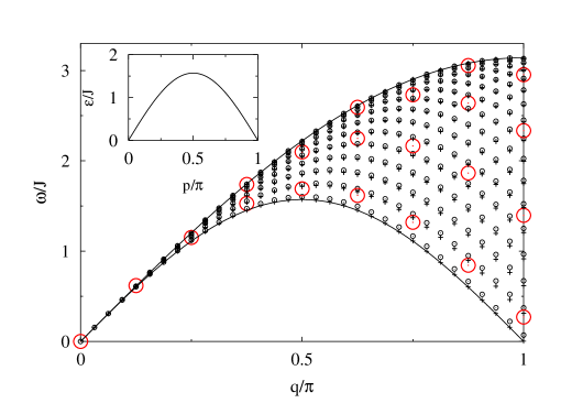
Figure 1: Energy versus wave number of all 2-spinon scattering states with $S_{T}^{z}=S_{T}=1$ at $q\geq 0$ for $N=64$ ($\circ$) in comparison with the corresponding free 2-spinon superpositions (+). The large red circles are 2-spinon data for $N=16$. The inset shows the energy-momentum relation (6) of the spinon quasi-particle.

The energies and wave numbers of the 2-spinon eigenstates for $N=64$ obtained via Bethe ansatz are represented by circles $(\circ)$ in Fig. 1, whereas the corresponding (fictitious) free 2-spinon superpositions with wave numbers $q=p_{1}+p_{2}$ and energy $\omega=\epsilon_{sp}(p_{1})+\epsilon_{sp}(p_{2})$ are shown as $(+)$ symbols. The upward displacement of the former relative to the latter is a measure of the positive spinon interaction energy caused by a predominently repulsive force acting between the two quasi-particles.

With increasing $N$, the scattering events between the two spinons in a 2-spinon state become scarcer at a rate inversely proportional to the distance covered by the quasi-particles between collisions. Consequently, the spinon interaction energy is expected to diminish $\propto N^{-1}$ (Problem 2). We conjecture that, asymptotically for large $N$, the spinon interaction energy in the 2-spinon scattering states, as defined by the expression

$$\Delta E_{2sp}^{(N)}(q)\equiv E_{2sp}^{(N)}(q)-\epsilon_{sp}(p_{1})-\epsilon_{sp}(p_{2})$$ (7)

with $q=p_{1}+p_{2}$ has the form

$$\Delta E_{2sp}^{(N)}(q)=e_{sp}(p_{1},p_{2})/N.$$ (8)

The quantity $e_{sp}(p_{1},p_{2})$ can then be attributed to a single 2-body collision between spinon quasi-particles traveling with momenta $p_{1},p_{2}$.

Figure 2: Scaled spinon interaction energy $e_{sp}(p_{1},p_{2})$ in the 2-spinon states for $N=64$ versus spinon momenta $p_{1},p_{2}$ (3D plot) and versus relative spinon momentum $|p_{1}-p_{2}|$ (inset).

The $N=64$ data for $e_{sp}(p_{1},p_{2})$ shown in Fig. 2 indicate that the interaction energy depends smoothly on the spinon momenta. It is observed to be smallest when both spinons have equal momenta. These states are near the upper boundary of the 2-spinon continuum. For fixed momentum $p_{1}>p_{2}$, the interaction energy is a monotonically decreasing function of $p_{2}$. Hence the largest interaction energy of states at fixed wave number $q$ is realized when the relative spinon momentum $|p_{1}-p_{2}|$ is a maximum. These states are near the lower boundary of the 2-spinon continuum.

At fixed $|p_{1}-p_{2}|$, the spinon interaction energy depends only weakly on the wave number $q$ of the 2-spinon state. Glancing at the data in Fig. 2 along the lines $p_{1}+p_{2}=$const. (direction of arrow), makes them collapse into a narrow band in the plane spanned by $e_{sp}$ and $|p_{1}-p_{2}|$ as shown in the inset to Fig. 2.

In Fig. 3 of part I we had illustrated the magnon interaction energy for 2-magnon scattering states. There the smallest interaction energy was realized when one of two magnons had infinite wavelength $(p_{2}=0)$. It then acted like a slightly rotated magnon vacuum in which the other magnon could move freely. A spinon, by contrast, becomes the strongest scatterer to another spinon when it has zero momentum.

The vanishing spinon interaction energy for $N\to\infty$ does not make the calculation of transition rates for the dynamic structure factor (3) a simple task. It was only recently that the exact 2-spinon part of $S_{zz}(q,\omega)$ at $h=0$ was evaluated for an infinite chain.KMB+97 The techniques used in that calculation, which involved generating the 2-spinon states from the spinon vacuum by means of spinon creation operators and expressing the spin fluctuation operator (2) in terms of spinon creation operators, are not readily generalizable to $h\neq 0$ (Problem 3a).

In nonzero field, a different approach is required. The ground state must be reinterpreted as the physical vacuum for a different species of quasi-particles. The spectral weight of $S_{zz}(q,\omega)$ will be dominated by scattering states of few quasi-particles from the new species, and the associated transition rates will be calculated via Bethe ansatz.

III Quasi-particles at $h\neq 0$: psinons

Increasing the magnetic field from $h=0$ to the saturation value $h=h_{S}=2J$, leaves all eigenvectors of (1) unaltered but shifts their energies at different rates. The ground state $|G\rangle$ changes in a sequence of level crossings, and the magnetization increases from $M_{z}=0$ to $M_{z}=N/2$ in units of one as discussed in part II. Every level crossing of that sequence adds two spinons to $|G\rangle$.

At $h\neq 0$ the number of spinons moving through the chain and scattering off each other is of O($N$). Scattering events are frequent. The spinon interaction energy does not vanish in the limit $N\to\infty$, because the density of spinons remains finite. Hence the spectrum of low-lying excitations cannot be reconstructed from the spinon energy-momentum relation (6).

If we start from the ground state $|F\rangle=|\uparrow\uparrow\cdots\uparrow\rangle$ at $h=h_{S}$ instead and decrease the the magnetic field gradually, we are also facing the problem of a runaway quasi-particle population. The state $|F\rangle$ is the vacuum of magnons, a species of quasi-particles with spin 1. Every reverse level crossing of the sequence considered previously adds one magnon as it removes two spinons. In the 2-magnon scattering states, which we had studied in part I, the role of individual magnons was just as clearly recognizable as the role of individual spinons in the 2-spinon scattering states depicted in Fig. 1. But in $|G\rangle$ at $0<h<h_{S}$ and in all low-lying excitations from that state, the number of magnons is macroscopic $(\propto N)$. The magnon interaction energy remains significant, which makes it impossible to infer spectral properties from the magnon energy-momentum relation (I5).

The ground-state wave function $|G\rangle$ at $0<h<h_{S}$ has spin quantum numbers $S_{T}=S_{T}^{z}=M_{z}$ ($0\leq M_{z}<N/2$) and is specified by the following set of $r=N/2-M_{z}$ Bethe quantum numbers:YY66a

$$\{I_{i}\}_{G}=\left\{-\frac{N}{4}+\frac{M_{z}}{2}+\frac{1}{2},\ldots,\frac{N}{4}-\frac{M_{z}}{2}-\frac{1}{2}\right\}.$$ (9)

Henceforth we treat $|G\rangle$, which can be interpreted as a state containing $N/2-M_{z}$ magnons or as a state containing $2M_{z}$ spinons, as a new physical vacuum and describe the dynamically relevant excitation spectrum from this reference state by modifying the uniform array (9) of Bethe quantum numbers systematically. For this purpose we consider the class $K_{r}$ of eigenstates whose Bethe quantum numbers comprise, for $0\leq r\leq N/2$ and $0\leq m\leq N/2-r$, all configurations

$$-\frac{r}{2}+\frac{1}{2}-m\leq I_{1}<I_{2}<\cdots<I_{r}\leq\frac{r}{2}-\frac{1}{2}+m.$$ (10)

We recall from part II that the $I_{i}$’s must be integer valued if $r$ is odd and half-integer valued if $r$ is even. Every class-$K_{r}$ eigenstate is represented by a real solution $\{z_{i}\}$ of the Bethe ansatz equation (II5),

$$N\phi(z_{i})=2\pi I_{i}+\sum_{j\neq i}\phi\bigl{[}(z_{i}-z_{j})/2\bigr{]},~{}i=1,\ldots,r,$$ (11)

with $\phi(z)\equiv 2\arctan z$. These solutions can be obtained iteratively via (II9) for fairly large systems. Every class-$K_{r}$ state at fixed integer quantum number $m$ $(0\leq m\leq M_{z})$ can be regarded as a scattering state of $m$ pairs of spinon-like particles, which we have named psinons.

At $M_{z}=0$ the psinon vacuum coincides with the spinon vacuum, both containing $N/2$ magnons. At saturation $(M_{z}=N/2)$, the psinon vacuum coincides with the magnon vacuum, a state containing $N$ spinons. The transformation of the psinon vacuum between the spinon vacuum and the magnon vacuum is illustrated in Fig. 3. It displays the configuration of Bethe quantum numbers for $|G\rangle$ in a system with $N=8$ and all values of $M_{z}$ realized between $h=0$ and $h=h_{S}$.

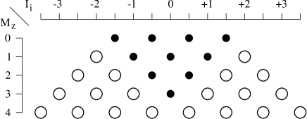
Figure 3: Psinon vacuum $|G\rangle$ for a chain of $N=8$ spins at magnetization $M_{z}=0,1,\ldots,4$. The position of the magnons $(\bullet)$ are determined by the set (9) of $I_{i}$’s and the positions of the spinons ($\bigcirc$) by the vacancies across the full range of the $I_{i}$’s allowed by (10).

The top row (spinon vacuum) corresponds to the top row in Fig. 3 of part II (albeit for different $N$). The second row is a particular state of the 2-spinon triplet set discussed in part II. The third row represents the psinon vacuum at half the saturation magnetization, $M_{z}/N=\frac{1}{4}$, the case we shall focus on in this paper. Here the psinon vacuum contains twice as many spinons as it contains magnons. The psinon vacuum in the fourth row corresponds to the highest-energy state of the 1-magnon branch described in part I. Trading the last magnon for a pair of spinons saturates $M_{z}$ and makes the psinon vacuum equal to the magnon vacuum (fifth row).

In the psinon vacuum $|G\rangle$, the only class-$K_{r}$ state with $m=0$, the magnons form a single array flanked by two arrays of spinons. Relaxing the constraint in (10) to $m=1$ yields the 2-psinon excitations. Generically, magnons now break into three clusters separated by the two innermost spinons, which now assume the role of psinons. The remaining $2M_{z}-2$ spinons stay sidelined.

In the 4-psinon states $(m=2)$, two additional spinons have been mobilized into psinons. By this prescription, we can systematically generate sets of $2m$-psinon excitations for $0\leq m\leq M_{z}$. From the psinon vacuum for $N=8,M_{z}=N/4=2$ depicted in the the third row of Fig. 3 we can thus generate the five 2-psinon states and the nine 4-psinon states identified in Fig. 4

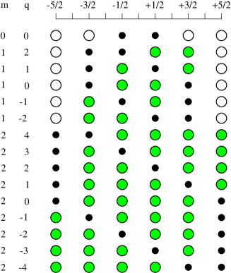
Figure 4: Psinon vacuum $(m=0)$ for $N=8,M_{z}=2$ and complete set of $2m$-psinon excitations with $m=1,2$ and wave numbers $q\equiv k-k_{G}$ (in units of $2\pi/N$). The positions of the magnons (small circles) are determined by the $I_{i}$’s and the positions of the spinons (large circles) by the $I_{i}$ vacancies. A subset of the spinons are the psinons (green circles).

Figure 5 shows energy versus wave number of all 2-psinon states at $M_{z}/N=\frac{1}{4}$ for system sizes $N=16$ (large red circles) and $N=64$ (small circles). In the limit $N\to\infty$, the 2-psinon states form a continuum in $(q,\omega)$-space with boundaries shown as blue lines. The 2-psinon spectrum is confined to $|q|\leq q_{s}$, where

$$q_{s}\equiv\pi(1-2M_{z}/N).$$ (12)

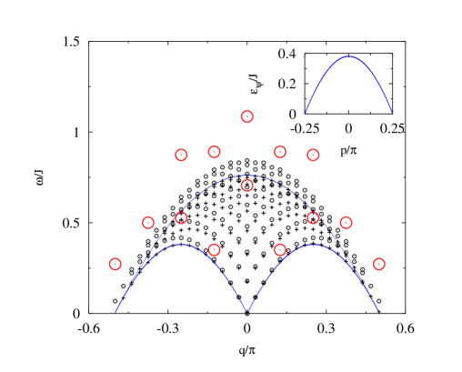
Figure 5: Spectrum in $(q,\omega)$-space of all 2-psinon scattering states at $M_{z}/N=\frac{1}{4}$ for $N=16$ (large red circles) and $N=64$ (small circles), the latter in comparison with the corresponding (fictitious) free 2-psinon states (+). The spectral range of the 2-psinon continuum for $N\to\infty$ (blue lines) are inferred from data for $N=2048$. The inset shows the psinon energy-momentum relation.

From the 2-psinon continuum boundaries we infer the psinon energy-momentum relation $\epsilon_{\psi}(p)$ shown in the inset, by the requirement that the wave number and the energy of every 2-psinon state for $N\to\infty$ can be accounted for by $q=p_{1}+p_{2}$ and $\omega=\epsilon_{\psi}(p_{1})+\epsilon_{\psi}(p_{2})$, respectively. The two arcs that make up the lower 2-psinon continuum boundary are then given by $\epsilon_{\psi}(q\pm\pi/4)$.

For finite $N$, the scattering of the two psinons in the 2-psinon states produces an interaction energy. In Fig. 5, this energy can again be measured by comparing the positions of the $N=64$ scattering states $(\circ)$ relative to the positions of the corresponding (fictitious) free 2-psinon states (+). The evidence from a comparison of the $N=64$ data in Figs. 3 and 5 is that the psinons at $M_{z}/N=\frac{1}{4}$ interact more strongly than the spinons at $M_{z}=0$ in chains of the same length. The interaction energy between two psinon quasi-particles in a 2-psinon scattering state can be investigated by the method used in Sec. II for spinon (Problem 4a). It again varies $\propto 1/N$.

Mobilizing two additional spinons into psinons makes the 4-psinon scattering states much more numerous than the 2-psinon states. Their number grows $\propto N^{4}$. In Fig. 6 we have plotted all 4-psinon states for $N=16$ and $N=64$ as well as the 4-spinon spectral range. The 4-psinon spectral threshold has the same shape as the 2-psinon lower boundary but extended periodically over the entire Brillouin zone. The upper 4-psinon boundary is obtained from the upper 2-psinon boundary by a scale transformation $(q\to 2q,\omega\to 2\omega)$.

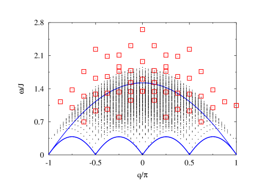
Figure 6: Spectrum in $(q,\omega)$-space of all 4-psinon excitations at $M_{z}=N/4$ for $N=16$ (red squares) and $N=64$ (dots). Also shown is the range of the 4-psinon states for $N\to\infty$ (blue lines) inferred from $N=2048$ data.

In both sets of states, the energy correction due to the psinon interaction is a $1/N$ effect. It fades away as the scattering events become less and less frequent in a system of increasing size. A comparison of finite-$N$ data in Figs. 5 and 6 shows that the finite-size energy correction caused by the psinon interaction is stronger in the 4-psinon states than in the 2-psinon states. The reason is the different rates at which scattering events between psinons occur.

At $M_{z}=0$ the 2-spinon excitations were found to dominate the spectral weight in the dynamic spin structure factor $S_{zz}(q,\omega)$.KMB+97 Our task here is to determine how the spectral weight of $S_{zz}(q,\omega)$ at $M_{z}\neq 0$ is distributed among the $2m$-psinon excitations. To accomplish it, we must calculate matrix elements.

IV Matrix elements

The Bethe ansatz has rarely been used for the purpose of calculating matrix elements. Most attempts at taking this approach have been deterred by the need of evaluating the sum ${\cal P}\in S_{r}$ over the $r!$ magnon permutations in the coefficients (I28) of the Bethe eigenvectors (I27):

$$|\psi\rangle=\sum_{1\leq n_{1}<\ldots<n_{r}\leq N}a(n_{1},\ldots,n_{r})|n_{1},\ldots,n_{r}\rangle,$$ (13)

$$a(n_{1},\ldots,n_{r})=\sum_{{\cal P}\in S_{r}}\exp\left(i\sum_{j=1}^{r}k_{{\cal P}j}n_{j}+\frac{i}{2}\sum_{i<j}\theta_{{\cal P}i{\cal P}j}\right).$$

The magnon momenta $\{k_{i}\}$ and the phase angles $\{\theta_{ij}\}$ are related via (II4) and (II5) to the solutions $\{z_{i}\}$ of the Bethe ansatz equations (11).

In the calculation of a single matrix element, a sum ${\cal P}\in S_{r}$ is evaluated many times, once for every coefficient $a(n_{1},\ldots,n_{r})$ of the two eigenvectors involved. Under these circumstances, it is imperative that the algorithm has rapid access to a table of permutations.

Table 1 describes a powerful recursive algorithm that generates all permutations of the numbers $1,2,\ldots,r$.Sedg92 These permutations are stored in the array ip of dimensionality $r!\times r$. The storage of this array in the RAM requires 645kB for $r=8$, 6.53MB for $r=9$, and 72.6MB for $r=10$.

Table 1: C++ code of a recursive algorithm that generates the $r!$ permutations of the numbers $1,2,\ldots,r$ and writes them into an array of dimensionality $r!\times r$. Each number is stored as a char or short, which is of size 2Bytes on an Intel processor (Ref. Sedg92 ).

void main()
{
  perm(0,r);
}
void perm(int k, int r)
{
 static long id=-1;
 static long rf=1;
 ip[0][k]=++id;
 if(id==r){
  for(int l=0;l<r;l++) ip[rf][l]=ip[0][l+1];
  rf++;
 }
 for(int t=1;t<=r;t++) if(ip[0][t]==0) perm(t,r);
 id--;
 ip[0][k]=0;
}

The computational effort of calculating any Bethe ansatz eigenvector (13) can be reduced considerably if we use the translational symmetry, ${\bf T}|\psi\rangle=e^{ik}|\psi\rangle$ (see part I). It is guaranteed by the relation

$$a(n_{1}+l,\ldots,n_{r}+l)=e^{ikl}a(n_{1},\ldots,n_{r})$$ (14)

between sets of coefficients pertaining to basis vectors that transform into each other under translation. Here the integers $n_{i}+l$ have to be used mod($N$). Translationally invariant basis vectors have the form

$$|j;k\rangle\equiv\frac{1}{\sqrt{d_{j}}}\sum_{l=0}^{d_{j}-1}e^{ilk}|j\rangle_{l},$$ (15)

where $|j\rangle_{l}\equiv{\bf T}^{l}|j\rangle_{0}=|n_{1}^{(j)}-l,\ldots,n_{r}^{(j)}-l\rangle$ and $1\leq N/d_{j}\leq N$ is an integer. The wave numbers $k$ realized in the set (15) are multiples mod($2\pi$) of $2\pi/d_{j}$.

The set of basis vectors $|j\rangle_{0}=|n_{1}^{(j)},\ldots,n_{r}^{(j)}\rangle,j=1,\ldots,d$, are the generators of the translationally invariant basis. The set of distinct vectors $|j;k\rangle$ for fixed $k$ is labeled $j\in{\cal J}_{k}\subseteq\{1,\ldots,d\}$. The rotationally invariant subspace for fixed $N/2-r$, which has dimensionality $D=N!/[r!(N-r)!]$, splits into $N$ translationally invariant subspaces of dimensionality $D_{k}$, one for each wave number $k=2\pi n/N,n=0,\ldots,N-1$. We have

$$D=\sum_{j=1}^{d}d_{j}=\sum_{0\leq k<2\pi}D_{k},~{}~{}D_{k}=\sum_{j\in{\cal J}_{k}}.$$ (16)

The Bethe eigenvector (13) expanded in this basis can thus be written in the form

$$|\psi\rangle=\sum_{j\in{\cal J}_{k}}a_{j}\sum_{l=0}^{d_{j}-1}e^{ilk}|j\rangle_{l}=\sum_{j=1}^{d}a_{j}\sum_{l=0}^{d_{j}-1}e^{ilk}|j\rangle_{l},$$ (17)

where the $a_{j}\equiv a(n_{1}^{(j)},\ldots,n_{r}^{(j)})$, the Bethe coefficients of the generator basis vectors $|j\rangle_{0}$, are the only ones that must be evaluated. The last expression of (17) holds because the Bethe coefficients $a_{j}$ of all generators $|j\rangle_{0}$ which do not occur in the set ${\cal J}_{k}$ are zero (Problem 5).

We calculate transition rates for the dynamic structure factor (3) in the form

$$|\langle G|S_{q}^{\mu}|\lambda\rangle|^{2}=\frac{|\langle\psi_{0}|S_{q}^{\mu}|\psi_{\lambda}\rangle|^{2}}{||\psi_{0}||^{2}||\psi_{\lambda}||^{2}},$$ (18)

where $|\psi_{0}\rangle,|\psi_{\lambda}\rangle$ are the (non-normalized) Bethe eigenvectors of the ground state and of one of the excited states from classes (i)-(vi), respectively. The norms are evaluated as follows:

$$||\psi||^{2}=\sum_{j=1}^{d}d_{j}|a_{j}|^{2}.$$ (19)

The matrix element $\langle\psi_{0}|S_{q}^{\mu}|\psi_{\lambda}\rangle$ is nonzero only if $q=k_{\lambda}-k_{0}+2\pi\mathbb{Z}$. For the fluctuation operator $S_{q}^{z}$ it can be evaluated in the form (Problem 6):

$$\langle\psi_{0}|S_{q}^{z}|\psi_{\lambda}\rangle\!=\!\frac{1}{\sqrt{N}}\sum_{j=1}^{d}\bar{a}_{j}^{(0)}a_{j}^{(\lambda)}\sum_{n=1}^{N}e^{iqn}\sum_{l=0}^{d_{j}-1}e^{ilq}{{}_{l}}\langle j|S_{n}^{z}|j\rangle_{l}.$$

The non-vanishing matrix elements $\langle\psi_{0}|S_{q}^{\pm}|\psi_{\lambda}\rangle$ needed for $S_{xx}(q,\omega)$ must also satisfy $q=k_{\lambda}-k_{0}+2\pi\mathbb{Z}$ and can be reduced to somewhat more complicated expressions involving elements ${}_{l_{0}}\langle j_{0}|S_{n}^{\pm}|j_{\lambda}\rangle_{l_{\lambda}}$ between basis vectors from different $S_{T}^{z}$ subspaces.

What are the memory requirements for the calculation of one such matrix element? Three arrays are needed for the basis vectors: long b[d], short nd[d] and, ndr[d][r]. The array b[d] holds the bit pattern of $|j\rangle_{0}$, nd[d] holds the numbers $d_{j}$, and in ndr[d][r] we store the $r$ numbers $n_{1}^{j},\ldots,n_{r}^{j}$ belonging to $|j\rangle_{0}$, i.e. b[j]. The arrays nd, ndr are not really necessary, since we can always calculate those numbers from b[j], but they help reduce the CPU-time. Finally, the two arrays complex psi[d] hold the coefficients $a_{j}$. Again, storing these numbers for multiple use cuts down on CPU time. In Table 2 we have summarized the memory requirements for several applications to the Heisenberg model (1).

Table 2: Memory (in kB) required for the calculation of matrix elements via Bethe ansatz on an Intel processor.

$N$	$r$	$d$	ip	b,nd,ndr	psi0,1	Total
12	6	80	9	1	3	13
14	7	246	71	5	8	83
16	8	810	645	18	26	689
18	9	2704	6532	65	87	6684
20	10	9252	72576	241	297	73112
16	4	116	0	2	3	6
20	5	776	1	12	25	38
24	6	5620	9	101	180	290
28	7	42288	71	846	1353	2270
32	8	328756	645	7232	10520	18398

With the exception of the case of $N=20,r=10$, we can compute the transition rates on a simple Pentium-PC with at least 32MB of memory. It is also worth mentioning that for the case $N=16,r=8$ no more than 1MB of memory is needed.

V Psinons and antipsinons

Which $2m$-psinon excitations have the largest spectral weight in $S_{zz}(q,\omega)$? We begin with a chain of $N=16$ spins at magnetization $M_{z}/N=\frac{1}{4}$, and explore the transition rates between the ground state $|G\rangle$ with $\{I_{i}\}_{G}=\frac{1}{2}\{-3,-1,+1,+3\}$, and all $2m$-psinon excitations for $m=0,1,2,3,4$.

First we calculate $\langle G|S_{q}^{z}|G\rangle$, which probes, for $q=0$, the ground-state magnetization induced by the magnetic field (Problem 7). Next we investigate the 2-psinon states. The $I_{i}$ configurations are shown in Fig. 7. The first row represents the psinon vacuum with its four magnons sandwiched by two sets of four spinons. The two innermost spinons (marked green) become psinons when at least one of them is moved to another position. In the rows underneath, the psinons are moved systematically across the array of magnons while the remaining spinons stay frozen in place. These eight configurations describe all 2-psinon states with wave number $0\leq q\leq\pi/2$.

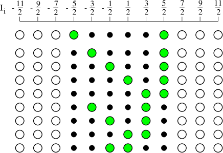
Figure 7: Psinon vacuum $|G\rangle$ for $N=16,M_{z}=4$ and 2-psinon states with $q\geq 0$. The $I_{i}$ values are marked by the positions of the magnons (small circles). The spinons (large circles) mark $I_{i}$-vacancies. A subset of the spinons are called psinons (green circles).

The $I_{i}$’s of the states shown in Fig. 7 and their wave numbers as inferred from (II8b) are listed in Table 3. Solving the Bethe ansatz equations (11) yields the ingredients needed to evaluate the energies via (II8a) and the transition rates via (IV), which are also listed in Table 3. We observe that almost all of the spectral weight is concentrated in the lowest excitation for any given wave number (lowest red circles in Fig. 5). In a macroscopic system, these states form the lower boundary of the 2-psinon continuum.

Table 3: Ground state and 2-psinon excitations for $N=16$, $M_{z}=4$, and wave numbers $q\equiv k-k_{G}\geq 0$ (in units of $2\pi/N$). The ground state has $k_{G}=0$ and $E_{G}=-11.5121346862$.

$2I_{i}$	$k-k_{G}$	$E-E_{G}$	$|\langle G|S_{q}^{z}|\lambda\rangle|^{2}$
$-3-1+1+3$	0	0.0000000000	1.0000000000
$-5-1+1+3$	1	0.3504534152	0.0484825989
$-5-3+1+3$	2	0.5271937189	0.0587154211
$-5-3-1+3$	3	0.5002699273	0.0773592284
$-5-3-1+1$	4	0.2722787522	0.1257902349
$-5-1+1+5$	0	0.7060324808	0.0000000000
$-5-3+1+5$	1	0.8908215652	0.0000064288
$-5-3-1+5$	2	0.8738923064	0.0000312622
$-5-3+3+5$	0	1.0855897189	0.0000000000

When we calculate the 4-spinon transition rates $|\langle G|S_{q}^{z}|\lambda\rangle|^{2}$, we find that most of their spectral weight is again carried by a single branch of excitations. The dynamically dominant 4-psinon states for $N=16$ are the eight lowest red squares in Fig. 6. For large $N$ they form a branch adjacent to the 2-psinon spectral threshold. An investigation of the $2m$-psinon states for $m=3,4,\ldots$ shows that there exists one dynamically dominant branch of $2m$-psinon excitations for $0<m<M_{z}$. All other $2m$-psinon excitations have transition rates that are smaller by at least two orders of magnitude at $q<\pi/2$ and still by more than one magnitude at $q\geq\pi/2$.

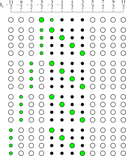
Figure 8: Psinon vacuum $|G\rangle$ for $N=16,M_{z}=4$ and set of $\psi\psi^{*}$ states with $0\leq q<\pi$. The $I_{i}$ are given by the positions of the magnons (small circles) in each row. The spinons (large circles) correspond to $I_{i}$-vacancies. The psinon $(\psi)$ and the antipsinon $(\psi^{*})$ are marked by a large and a small grey circle, respectively.

Figure 8 shows the $I_{i}$ configurations of the four dynamically dominant $2m$-psinon branches for $N=16$. Each branch (at $q>0$) consists of $N/2-M_{z}=4$ states. An interesting pattern emerges, which is indicative of the nature of the relevant quasi-particles in these dynamically dominant collective excitations. The two relevant quasi-particles are highlighted by green circles.

We identify one of the two quasi-particles as a psinon (large green circle) as before and the other one as a new quasi-particle (small green circle). The latter is represented by a hole in what was one of two spinon arrays of the psinon vacuum. Instead of focusing on the cascade of psinons (mobile spinons) which this hole has knocked out of the psinon vacuum, we focus on the hole itself, which has properties commonly attributed to antiparticles. The psinon $(\psi)$ and the antipsinon $(\psi^{*})$ exist in disjunct parts of the psinon vacuum, namely in the magnon and spinon arrays, respectively. When they cross paths at the border of the two arrays, they undergo a mutual annihilation, represented by the step from the second row to the top row in Fig. 8.

The large red circles in Fig. 9 represent all $\psi\psi^{*}$ states at $q>0$ for $N=16$ as specified in Fig. 8. There are four branches ($m=1,\ldots,4$ from bottom to top) with four states each. Also shown in Fig. 9 are the $\psi\psi^{*}$ states for $N=64$ (small circles). The solid lines are inferred from $\psi\psi^{*}$ data for $N=2048$ and represent the boundaries of the $\psi\psi^{*}$ continuum in the limit $N\to\infty$.

Why have we chosen to interpret the small green circle in Fig. 8 as an antipsinon and not as a magnon? Either choice is valid but we must heed the fact that antipsinons and magnons live in different physical vacua.

When we interpret the small green circle as a magnon, then it coexists in the magnon vacuum with a macroscopic number of fellow magnons (small black circles). The collective excitations must then be viewed as containing a finite density of magnons (for $N\to\infty$), in which the magnon interaction remains energetically significant for scattering states. The nonvanishing interaction energy obscures the role of individual magnons.

On the other hand, when we interpret the small green circle as an antipsinon, then it lives in the psinon vacuum, i.e. almost in isolation. The only other particle present is a psinon (large green circle). In the limit $N\to\infty$, the interaction energy in a psinon-antipsinon $(\psi\psi^{*})$ scattering state vanishes.

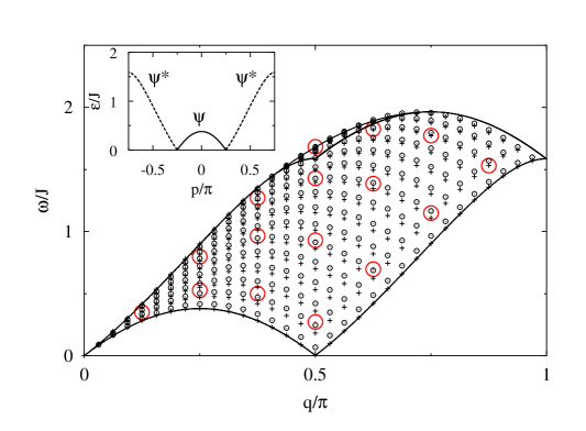
Figure 9: Energy versus wave number of all $\psi\psi^{*}$ scattering states at $M_{z}/N=\frac{1}{4}$ and $q\geq 0$ for $N=64$ ($\circ$) in comparison with the corresponding free $\psi\psi^{*}$ states $(+)$. Also shown are the $\psi\psi^{*}$ states for $N=16$ (large red circles). The inset shows the energy-momentum relations of the psinon $(0\leq|p|\leq\pi/4)$ and the antipsinon $(\pi/4\leq|p|\leq 3\pi/4)$.

The energy-momentum relations of the two quasi-particles (see inset to Fig. 9) can be accurately inferred from $N=2048$ data for the spectral thresholds of the $\psi\psi^{*}$ states. The psinon dispersion $\epsilon_{\psi}(p)$ is confined to the interval at $0\leq|p|\leq\pi/4$ (solid line) and the antipsinon dispersion $\epsilon_{\psi^{*}}(p)$ to $\pi/4\leq|p|\leq 3\pi/4$ (dashed line). The lower boundary of the $\psi\psi^{*}$ continuum is defined by collective states in which one of the two particles has zero energy: the antipsinon for $0\leq|q|\leq\pi/2$ and the psinon for $\pi/2\leq|q|\leq\pi$. The upper boundary consists of three distinct segments.

For $0\leq q\lesssim 0.3935$ the highest $\psi\psi^{*}$ state is made up of a zero-energy psinon with momentum $p_{\psi}=-\pi/4$ and an antipsinon with momentum $p_{\psi^{*}}=\pi/4+q$. Likewise, for $3\pi/4\leq q\leq\pi$, the states along the upper continuum boundary are made up of a maximum-energy antipsinon (with $p_{\psi^{*}}=3\pi/4$) and a psinon with $p_{\psi}=-3\pi/4+q$. In these intervals, the shape of the continuum boundary is that of $\epsilon_{\psi}$ or $\epsilon_{\psi^{*}}$.

When the two delimiting curves are extended into the middle interval, $0.3935\lesssim q\leq 3\pi/4$, they join in a cusp singularity at $q=\pi/2$. Here the maximum of $\epsilon_{\psi}(p_{\psi})+\epsilon_{\psi^{*}}(p_{\psi^{*}})$ subject to the constraint $p_{\psi}+p_{\psi^{*}}=q$ does not occur at the endpoint of any quasi-particle dispersion curve. Consequently, the $\psi\psi^{*}$ continuum is partially folded about the upper boundary along the middle segment as is evident in Fig. 9.

The $(+)$ symbols in Fig. 9 represent $N=64$ data of free $\psi\psi^{*}$ superpositions generated from the $\psi$ and $\psi^{*}$ energy-momentum relations. The vertical displacement of any $(\circ)$ from the associated $(+)$ thus reflects the interaction energy between the two quasi-particles in a $\psi\psi^{*}$ state. A comparison of the $N=64$ data in Figs. 7 and 9 shows that for the most part the $\psi\psi^{*}$ interaction energy is smaller than the $\psi\psi$ interaction energy (Problem 4b).

The lower boundary of the $\psi\psi^{*}$ continuum touches down to zero frequency at $q=0$ and $q=q_{s}\equiv\pi/4$, which is a special case of Eq. (12). Between $q_{s}$ and $\pi$, it rises monotonically and reaches the value $E-E_{G}=h$ for $N\to\infty$ (Problem 8). A direct observation of the zero-frequency mode at $q_{s}$ was made in a neutron scattering experiment on copper benzoate.DHR+97

When we lower $M_{z}$, the soft mode at $q_{s}$ moves to the right, the number of $2m$-psinon branches contributing to the $\psi\psi^{*}$ continuum shrinks but each branch gains additional states. At $M_{z}=1$ we are left with one 2-psinon branch extending over the interior of the entire Brillouin zone. This branch is equal to the lowest branch of 2-spinon states with dispersion $\epsilon_{L}(q)$, Eq. (5). At $M_{z}=0$ the $\psi\psi^{*}$ excitations disappear altogether.

When we increase $M_{z}$ toward the saturation value, the zero-frequency mode moves to the left, and the number of $2m$-psinon branches increases but each branch becomes shorter. At $M_{z}=N/2-1$, the two-parameter set collapses into a one-parameter set consisting of one $2m$-psinon state each for $m=1,2,\ldots,N/2-1$. In part I these states were identified as 1-magnon excitations with dispersion $\epsilon_{1}(q)=J(1-\cos q)$ (Problem 9).

VI Lineshapes

What have we accomplished thus far and what remains to be done? We have identified the model system and the dynamical quantity which is relevant for the interpretation of inelastic neutron scattering data (Sec. I). We have configured the ground state at $h\neq 0$ as the vacuum for psinon quasi-particles and related it to the ground state at $h=0$, the spinon vacuum (Secs. II and III). We have introduced a method of calculating matrix elements for the dynamic spin structure factor $S_{zz}(q,\omega)$ via the Bethe ansatz (Sec. IV). We have it to identify among all the $2m$-psinon states one continuum of collective excitations which contributes most of the spectral weight to $S_{zz}(q,\omega)$: the $\psi\psi^{*}$ states (Sec. V). Here we use the spectral information and the transition rates, all evaluated via Bethe ansatz, to calculate the lineshapes relevant for fixed-$q$ scans in the neutron scattering experiment.

To finish the task, we exploit key properties of transition rates and densities of states of sets of excitations that form two-parameter continua in $(q,\omega)$-space for $N\to\infty$. The two parameters are quantum numbers of the $\psi$ and $\psi^{*}$ quasi-particles, e.g. the positions $\nu,\nu^{*}$ on the $I_{i}$-scale of Fig. 8 of the two green circles. For $N\to\infty$, the scaled quantum numbers $\nu/N,\nu^{*}/N$ become piecewise smooth functions of the physical parameters $q,\omega$. The $\psi\psi^{*}$ transition rates (scaled by $N$) then turn into a continuous function $M_{zz}^{\psi\psi^{*}}(q,\omega)$ and the $\psi\psi^{*}$ density of states (scaled by $N^{-1}$) into a continuous function $D_{zz}^{\psi\psi^{*}}(q,\omega)$. The $\psi\psi^{*}$ spectral-weight distribution is the product $S_{zz}^{\psi\psi^{*}}(q,\omega)=D_{zz}^{\psi\psi^{*}}(q,\omega)M_{zz}^{\psi\psi^{*}}(q,\omega)$.

In the following, we consider the case $q=\pi/2$, where the $\psi\psi^{*}$ continuum is gapless. The density of $\psi\psi^{*}$ states is generated from $N=2048$ data of

$$D_{zz}^{\psi\psi^{*}}(q,\omega_{\nu^{*}})\equiv\frac{2\pi/N}{\omega_{\nu^{*}+1}-\omega_{\nu^{*}}},$$ (21)

where $\nu^{*}=m$ marks the antipsinon quantum number in the $\psi\psi^{*}$ continuum. The psinon quantum number $\nu$ is adjusted to keep the wave number $q$ of the $\psi\psi^{*}$ state fixed. The resulting ordered sequence of levels substituted into (21) yields the graph shown in Fig. 10(a) (Problem 3b).

The function $D_{zz}^{\psi\psi^{*}}(\pi/2,\omega_{\nu^{*}})$ rises from a nonzero value at $\omega=0$ slowly up to near the upper boundary, where it bends into a divergence. A log-log plot of the data near the upper band edge reveals that it is a square-root divergence. Finite-$N$ data over a range of system sizes for the scaled transition rates

$$M_{zz}^{\psi\psi^{*}}(q,\omega_{\nu^{*}})\equiv N|\langle G|S_{q}^{z}|\nu^{*}\rangle|^{2}$$ (22)

with $q=\pi/2$ are shown in Fig. 10(b). They confirm the smoothness of $M_{zz}^{\psi\psi^{*}}(\pi/2,\omega)$. It has a monotonic $\omega$-dependence with a divergence at $\omega=0$ and a cusp singularity at the upper boundary $\omega_{U}\simeq 1.679J$ of the $\psi\psi^{*}$ continuum.

Figure 10: (a) Density of $\psi\psi^{*}$ states at $q=\pi/2$ evaluated via (21) from Bethe ansatz data for $N=2048$. (b) Transition rates (22) between the psinon vacuum and the $\psi\psi^{*}$ states at $q=\pi/2$ for $N=12,16,20,24,28,32$. (c) Lineshape at $q=\pi/2$ of the $\psi\psi^{*}$ contribution to $S_{zz}(q,\omega)$. All results pertain to $M_{z}/N=\frac{1}{4}$.

The product of the transition rate function and the (interpolated) density of states is shown in Fig. 10(c). The curve fitted through the data points represents the $\psi\psi^{*}$ lineshape of $S_{zz}(q,\omega)$ at $q=\pi/2$. Its most distinctive feature is the two-peak structure caused by divergent transition rates and a divergent density of states at the lower and upper band edges, respectively. The divergence at $\omega=0$ is a power law, $~{}\omega^{-\alpha}$, with an exponent that is exactly known from field theoretic studies:Hald80 $\alpha=0.4688\ldots$. The strength of the divergence at $\omega_{U}$ depends on whether or not the cusp singularity of $M_{zz}^{\psi\psi^{*}}(\pi/2,\omega)$ starts from zero at $\omega=\omega_{U}$ (Problem 10).

The observability of this lineshape in a neutron scattering experiment also depends on the relative $\psi\psi^{*}$ contribution to the integrated intensity of $S_{zz}(\pi/2,\omega)$. With the tools developed here, we can show that the $\psi\psi^{*}$ states contribute at least 93% of the spectral weight at this particular wave number (Problem 11). A more complete analysis of the lineshapes and the integrated intensity of $S_{zz}(q,\omega)$ for the model system at $M_{z}/N=\frac{1}{4}$ can be found elsewhere.KM00

Where do we go from here with this series of tutorial papers on the Bethe ansatz? In the next installment, we plan on making the exchange interaction in (1) uniaxially anisotropic. This well set the stage for the investigation of the following topics. Like the magnetic field, the anisotropy is a useful continuous parameter which brings about interesting effects in the excitation spectrum of the spin chain. Unlike the former, the latter does affect the wave functions of the system. The Bethe ansatz offers us a close-up look into these changes. Foremost among them is the transformation of 2-spinon scattering states into 2-spinon bound states and the consequent changes of their roles in dynamic structure factors.

VII Problems for further study

(1) (a) Show that if you subject $\langle S_{l}^{\mu}(t)S_{l^{\prime}}^{\mu}(0)\rangle$, $\mu=x,y,z$, at $T=0$ for a cyclic chain of $N$ sites to a space-time Fourier transform, $S_{\mu\mu}(q,\omega)=N^{-1}\sum_{ll^{\prime}}e^{iq(l-l^{\prime})}\int_{-\infty}^{+\infty}dt\,e^{i\omega t}\langle S_{l}^{\mu}(t)S_{l^{\prime}}^{\mu}(0)\rangle$, you end up with expression (3). (b) Show that the static structure factor $S_{\mu\mu}(q)\equiv\langle G|S_{q}^{\mu}S_{-q}^{\mu}|G\rangle$ as obtained from a single diagonal matrix element is equal to the integrated intensity of (3), $\int_{-\infty}^{+\infty}(d\omega/2\pi)S_{\mu\mu}(q,\omega)=\sum_{m}|\langle G|S_{q}^{\mu}|m\rangle|^{2}$ as obtained from a sum of off-diagonal matrix elements.

(2) Consider the lowest-lying 2-spinon excitation at $q=\pi/2$. Find the pattern of its Bethe quantum numbers $I_{i}$ for arbitrary $N$. Use Eq. (II9) to calculate the excitation energy $E_{\pi/2}(N)$ of that state for a range of system sizes. Plot the spinon interaction energy $E_{\pi/2}(N)-\pi J/2$ versus $1/N$ to verify the $N$-dependence suggested in the text. Repeat the same task for the lowest 2-spinon excitation at $q=\pi$. Here the reference energy is zero. Verify the exact resultHHM95 $E_{\pi}(N)\sim\alpha/N$, $\alpha=\pi^{2}/2$ for this excitation via extrapolation.

(3) (a) Use the result (II30), $\epsilon(q,\bar{q})=\pi J|\sin\frac{1}{2}q\cos\bar{q}|$, $0\leq\bar{q}\leq q$, for the 2-spinon spectrum at some wave number $0\leq q\leq\pi$ to calculate the 2-spinon density of states analytically via $D(q,\omega)=\int_{0}^{q}d\bar{q}\delta\left(\omega-\epsilon(q,\bar{q})\right)$. The result $D(q,\omega)=\left[\epsilon_{U}^{2}(q)-\omega^{2}\right]^{-1/2}$ for $\epsilon_{L}(q)<\omega\epsilon_{U}(q)$ is then to be multiplied by the exact transition rate function $M(q,\omega)$ derived in Ref. KMB+97, to produce the exact 2-spinon part of $S_{zz}(q\omega)$. (b) Reproduce the analytic result for $D(\pi,\omega)$ computationally from finite-$N$ data via Eq. (21) with $\nu^{*}$ now labelling the 2-spinon states at $q=\pi$ in order of increasing energy.

(4) (a) For sufficiently large $N$ the psinon interaction energy in the 2-psinon scattering states is of the form $\Delta E_{2\psi}^{(N)}(q)\simeq e_{\psi}(p_{1},p_{2})/N$, where $q=p_{1}+p_{2}$ and $e_{\psi}(p_{1},p_{2})$ depends smoothly on the psinon momenta $p_{1},p_{2}$. Since we do not know the psinon energy-momentum relation $\epsilon_{\psi}(p)$ analytically, use the 2-psinon lower boundary for $N^{*}\gg N$ as an approximation for $\epsilon_{\psi}(p\pm\pi/4)$ in $\Delta E_{2\psi}^{(N)}(q)\equiv E_{2\psi}^{(N)}(q)-\epsilon_{\psi}(p_{1})-\epsilon_{\psi}(p_{2})$. Plot $N\Delta E_{2\psi}^{(N)}(q)$ versus $(p_{1},p_{2})$ for 2-psinon states of systems with $N^{*}\gg N\gg 1$ judiciously chosen. Compare the properties of the newly found function $e_{\psi}(p_{1},p_{2})$ with those of the function $e_{sp}(p_{1},p_{2})$ established in Fig. 2 for spinons. (b) Carry out the same procedure for the $\psi\psi^{*}$ states. The lowest branch of states is the same as in (a). Compare the trends in quasi-particle interaction energies with increasing energy of the 2-psinon states and $\psi\psi^{*}$ states.

(5) Identify a complete set of generators $|j\rangle_{0},j=1,\ldots,d$ for the (15) in the subspace $N=6,r=3$. Verify that the $d_{j}$ associated with these generators add up to $D$. Establish the sets ${\mathcal{J}}_{k}$ for $k=0,\pi/3,\ldots,5\pi/3$. Show that the $D_{k}$ add up to $D$. Calculate the Bethe coefficients $a_{j}$ of the $d=4$ generators for all $D=20$ solutions of the Bethe ansatz equations by using the data from Table IV of part I. Show that all $a_{j}$ with $j\notin{\mathcal{J}}_{k}$ vanish.

(6) Use the results of Problem 5 to calculate (for $N=6$, $r=3$) the structure factor $\langle G|S_{q}^{\mu}S_{-q}^{\mu}|G\rangle$ and the transition rates $|\langle G|S_{q}^{\mu}|m\rangle|^{2}$. Show that these data satisfy the general result of Problem 1(b).

(7) Show that $|\langle G|S_{q=0}^{z}|G\rangle|^{2}=M_{z}^{2}/N$ and use this result to test your computer program which calculates transition rates from Bethe wave functions.

(8) The $2m$-psinon branch $(0<m\leq M_{z})$ of the $\psi\psi^{*}$ continuum at $q>0$ is specified by the $r=N/2-M_{z}$ Bethe quantum numbers $I_{1}=-N/4+M_{z}/2+\frac{1}{2}-m$, $-N/4+M_{z}/2+\frac{1}{2}\leq I_{2}<\ldots<I_{R}\leq N/4-M_{z}/2-\frac{1}{2}$. (a) Identify the Bethe quantum numbers of the $\psi\psi^{*}$ state with the lowest energy above the ground state $|G\rangle$. Show that the wave number of this state is $k-k_{G}=\pi(1-2M_{z}/N)$. Show by numerical extrapolation of finite-$N$ data that its excitation energy tends to zero as $N\to\infty$. (b) Identify the Bethe quantum numbers of the sole $\psi\psi^{*}$ state with $q=\pi-2\pi/N$. Plotting the excitation energy of this state versus $M_{z}/N$ yields a set of data points that converges, as $N\to\infty$, toward the inverse magnetization curve $h(M_{z})$.

(9) Use the exact 1-magnon wave functions (I6) with Bethe coefficients (I8) in expressions (18)-(IV) to calculate the $\psi\psi^{*}$ transition rates $|\langle G|S_{q}^{z}|\lambda\rangle|^{2}$ for $M_{z}=N/2-1$ and arbitrary $N$. Note the different $N$-dependence for $q=0$ and $q\neq 0$. Show that the relative $\psi\psi^{*}$ spectral weight in $S_{zz}(q,\omega)$ is 100%, but the absolute intensity for $q\neq 0$ is only of O($N^{-1}$).

(10) (a) Use the lowest-energy excitation for $N=12,16,\ldots,32$ to perform a nonlinear fit of the expression $M_{zz}^{\psi\bar{\psi}}(\pi/2,\omega_{\bar{\nu}})\sim a_{1}+a_{2}\omega^{-\alpha}$ and compare the exponent value thus obtained with the field-theoretic prediction quoted in the text. (b) Use all data at $\hbar\omega/J>1$ to fit the expression $M_{zz}^{\psi\bar{\psi}}(\pi/2,\omega_{\bar{\nu}})\sim b_{1}+b_{2}(\omega_{U}-\omega)^{\beta}$. Perform an alternative fit in which $b_{1}$ is forcibly set equal to zero.

(11) For fixed $N$, the integrated intensity is the expectation value $\langle G|S_{\pi/2}^{z}S_{\pi/2}^{z}|G\rangle$ and the $\psi\psi^{*}$ part thereof the sum of transition rates $\sum_{\nu^{*}=1}^{N/4}|\langle G|S_{\pi/2}^{z}|\nu^{*}\rangle|^{2}$ as worked out in Problem 1. Evaluate these quantities from the Bethe wave functions for $N=12,16,\ldots$ and extrapolate the ratio find the relative spectral weight of the $\psi\psi^{*}$ excitations in $S_{zz}(\pi/2,\omega)$.

- (1) P. R. Hammar, M. B. Stone, D. H. Reich, C. Broholm, P. J. Gibson, M. T. nad C. P. Landee, and M. Oshikawa, Phys. Rev. B 59, 1008 (1999).
- (2) S. E. Nagler, D. A. Tennant, R. A. Cowley, T. G. Perring, and S. K. Satija, Phys. Rev. B 44, 12361 (1991).
- (3) E. Balcar, S. W. Lovesey, Theory of Magnetic Neutron and Photon Scattering. Oxford University Press, 1989.
- (4) Frontiers of Neutron Scattering. Proceedings of the 7th Summer School on Neutron Scattering, Ed. A. Furrer, World Scientific 2000.
- (5) M. Karbach and G. Müller, Comp. in Phys. 11, 36 (1997).
- (6) M. Karbach, K. Hu, and G. Müller, Comp. in Phys. 12, 565 (1998).
- (7) L. D. Faddeev and L. A. Takhtajan, Phys. Lett. A85, 375 (1981).
- (8) J. Des Cloizeaux and J. J. Pearson, Phys. Rev. 128, 2131 (1962).
- (9) T. Yamada, Prog. Theor. Phys. 41, 880 (1969).
- (10) M. Karbach, G. Müller, A. H. Bougourzi, A. Fledderjohann, and K.-H. Mütter, Phys. Rev. B p. 12510 (1997).
- (11) C. N. Yang and C. P. Yang, Phys. Rev. 150, 321 (1966).
- (12) R. Sedgewick, Algorithms in C++ (Addison Wesley, Reading, Massachusetts, 1992).
- (13) D. C. Dender, P. R. Hammar, D. C. Reich, C. Broholm, and G. Aeppli, Phys. Rev. Lett. 79, 1750 (1997).
- (14) F. D. M. Haldane, Phys. Rev. Lett. 45, 1358 (1980).
- (15) M. Karbach and G. Müller, [cond-mat/0005174].
- (16) K. Hallberg, P. Horsch, and G. Martínez, Phys. Rev. B 52, R719 (1995).