Luttinger liquid behavior in metallic carbon nanotubes

Abstract

Coulomb interaction effects have pronounced consequences in carbon nanotubes due to their 1D nature. In particular, correlations imply the breakdown of Fermi liquid theory and typically lead to Luttinger liquid behavior characterized by pronounced power-law suppression of the transport current and the density of states, and spin-charge separation. This paper provides a review of the current understanding of non-Fermi liquid effects in metallic single-wall nanotubes (SWNTs). We provide a self-contained theoretical discussion of electron-electron interaction effects and show that the tunneling density of states exhibits power-law behavior. The power-law exponent depends on the interaction strength parameter $g$ and on the geometry of the setup. We then show that these features are observed experimentally by measuring the tunneling conductance of SWNTs as a function of temperature and voltage. These tunneling experiments are obtained by contacting metallic SWNTs to two nanofabricated gold electrodes. Electrostatic force microscopy (EFM) measurements show that the measured resistance is due to the contact resistance from the transport barrier formed at the electrode/nanotube junction. These EFM measurements show also the ballistic nature of transport in these SWNTs. While charge transport can be nicely attributed to Luttinger liquid behavior, spin-charge separation has not been observed so far. We briefly describe a transport experiment that could provide direct evidence for spin-charge separation.

1 Introduction

The electronic properties of one-dimensional (1D) metals have attracted considerable attention for fifty years by now. Starting with the work of Tomonaga in 1950 tomonaga and later by Luttinger luttinger , it has become clear that the electron-electron interaction destroys the sharp Fermi surface and leads to a breakdown of the ubiquituous Fermi liquid theory pioneered by Landau landau . This breakdown is signalled by a vanishing quasiparticle weight $Z_{F}$ in the presence of arbitrarily weak interactions. The resulting non-Fermi liquid state is commonly called Luttinger liquid (LL), or sometimes Tomonaga-Luttinger liquid. The name “Luttinger liquid” was coined by Haldane haldane to describe the universal low-energy properties of one-dimensional conductors. Universality means that the physical properties do not depend on details of the model, the interaction potential, etc., but instead are only characterized by a few parameters (critical exponents). The range of validity of the LL model is usually set by $E\ll D$, where $D$ is an electronic bandwidth parameter and $E$ is the relevant energy scale, namely either the thermal scale $k_{B}T$ or the applied voltage $eV$. Quite remarkably, the LL concept is believed to hold for arbitrary statistical properties of the particles, e.g. both for fermions and bosons. It provides a paradigm for non-Fermi liquid physics and may have some relevance also for higher-dimensional systems, e.g. in relation to high-temperature superconductivity.

In the model studied by Tomonaga and Luttinger, a special dispersion relation for the noninteracting problem was assumed, where one linearizes around the two Fermi vectors $\pm k_{F}$ present in 1D. At sufficiently low energy scales, such a procedure should clearly be possible. In fact, we will see below that in a nanotube the dispersion relation is highly linear anyways. Assuming a linear dispersion relation composed of left- and right-moving particles with Fermi velocity $v_{F}$, one can equivalently express the noninteracting problem in terms of collective plasmon (density wave) excitations. Technically, in the “bosonization” language bosonization , for the simplest case of a spinless single-channel system, these bosonic excitations can be expressed in terms of a displacement field $\theta(x)$ such that the density fluctuations are $\rho(x)=\pi^{-1/2}\partial_{x}\theta(x)$. Electron-electron interactions then describe a bilinear coupling of these density fluctuations, and therefore the full interacting problem can be written as a free theory in the displacement field:

$$H=\frac{\hbar v_{F}}{2}\int dx\left(\Pi^{2}(x)+\frac{1}{g^{2}}[\partial_{x}\theta(x)]^{2}\right)\;,$$ (1)

where $\Pi(x)$ is the canonical momentum to the field $\theta(x)$. In the long-wavelength limit, one can approximate the Fourier transform $\widetilde{V}(k)$ of the 1D interaction potential by a constant $V_{0}=\widetilde{V}(0)-\widetilde{V}(2k_{F})$, and the dimensionless $g$ parameter in Eq. (1) is given by

$$g=[1+V_{0}/\pi\hbar v_{F}]^{-1/2}\;.$$ (2)

Note that for repulsive interactions we always have $g<1$, with small $g$ meaning strong interactions. The limit $g=1$ describes the Fermi gas (not a Fermi liquid), and the limit $g\to 0$ leads to a classical Wigner crystal. The model (1) is equivalent to a set of harmonic oscillators and can therefore be solved exactly. The physical interpretation can be elucidated by the use of the bosonization formula for the electron operator itself bosonization . Thereby, the creation operator for a right- or left-moving electron ($r=R/L=\pm$) can be written in the form

$$\psi_{r}(x)\simeq\frac{1}{\sqrt{2\pi a}}\exp\Bigl{(}irk_{F}x+ir\sqrt{\pi}\theta(x)+i\sqrt{\pi}\int^{x}dx^{\prime}\Pi(x^{\prime})\Bigr{)}\;,$$ (3)

where $a\approx 1/k_{F}$ is a lattice constant. Using this expression, it is a simple matter to show that the sharp $T=0$ Fermi surface is smeared out for $g<1$, with interaction-dependent power laws close to $k_{F}$. Physically, this is because the electron is an unstable particle and spontaneously decays into collective plasmon modes. Including the spin-1/2 degree of freedom, one finds that the spin and charge plasmons also decouple and moreover propagate with different velocities $v_{c}\neq v_{s}$. This phenomenon is called spin-charge separation and implies that the spin and charge degrees of freedom of an electron brought into a LL will spatially separate. Note that in a Fermi liquid $v_{c}=v_{s}$ and therefore this characteristic feature will not show up. Spin-charge separation is intrinsically a dynamical phenomenon outside the scope of thermodynamics.

An interesting and closely related issue concerns the fractionalized stable excitations of the LL. While it is easy to establish the spin-charge separation phenomenon in the bosonic plasmon basis, the nature of the expected fundamental “quasiparticles” with fractional statistics, similar to the famous Laughlin quasiparticles in the fractional quantum Hall (FQH) effect, is less clear. In a 1D Hubbard chain, which is known to be a realization of the LL at low temperatures, well-defined spinon and holon excitations exist. For a spinless system, one can establish that quasiparticles scattered by a weak impurity potential have fractional charge $ge$ and a statistical angle $\pi g$ mpa . Remarkably, the fractional charge can have any – even irrational – value. Furthermore, for the topology of a LL on a ring, a complete characterization of the universal LL theory in terms of fractional-statistics quasiparticles has been provided recently pham .

In view of this discussion, it is understandable that, for many decades, experimentalists have attempted to find LL behavior. In the 1970s, the key interest was focused on quasi-1D organic chain compounds voit , where LL behavior is hard to establish because of complicated 1D-3D crossover phenomena and additional phase transitions into other states. The interest was revived a few years ago, when experimental observations of LL behavior for transport in semiconductor quantum wires tarucha ; auslaender and for edge states in FQH bars milliken ; chang were reported. Shortly after the theoretical prediction of LL behavior in metallic carbon nanotubes egger ; egger2 , the to-date perhaps cleanest experimental observations of LL behavior were established in transport experiments for single-wall nanotubes (SWNTs) bockrath ; yao . The theory along with the experiments of Ref. bockrath will be presented below. By now, there are also several other theoretical proposals for probing the LL state in bulk systems, e.g. by investigating the tunneling density of states (TDOS) of a 3D metal in an ultra-strong magnetic field glaz , or by studying 2D arrays of regularly stacked nanotubes kane .

Carbon nanotubes were discovered in 1991 by Iijima tube91 and have enjoyed exponentially increasing interest since then. The current status of the field has been summarized in a recent Physics World issue pworld , see also Ref. dekker . Ignoring the end structure, one may think of a SWNT as a graphene sheet, i.e. a 2D honeycomb lattice made up of C atoms, that is wrapped onto a cylinder, with typical radius of order 1-2 nm and length of several microns. Depending on the helicity of the wrapping, the resulting SWNT is either semiconducting or metallic. In our experimental setup discussed in Sec. 3, these two behaviors can be distinguished as follows. When the conductance $G$ of the tube is measured as a function of a gate voltage $V_{g}$, $G$ is virtually independent of $V_{g}$ for metal tubes, while $G$ varies exponentially with $V_{g}$ for semiconducting tubes. The discussion in this paper is limited to transport through metallic SWNTs, where LL behavior can be expected.

From the special band structure of a graphene sheet pworld , one arrives at the characteristic dispersion relation of a metallic SWNT shown in Figure 1. This band structure exhibits two Fermi points $\alpha=\pm$ with a right- and a left-moving ($r=R/L=\pm$) branch around each Fermi point. These branches are highly linear with Fermi velocity $v_{F}\approx 8\times 10^{5}$ m/s. The R- and L-movers arise as linear combinations of the $p=\pm$ sublattice states reflecting the two C atoms in the basis of the honeycomb lattice. The dispersion relation depicted in Fig. 1 holds for energy scales $E<D$, with the bandwidth cutoff scale $D\approx\hbar v_{F}/R$ for tube radius $R$. For typical SWNTs, $D$ will be of the order 1 eV. The large overall energy scale together with the structural stability of SWNTs explain their unique potential for revealing LL physics. In contrast to conventional systems, e.g. semiconductor quantum wires, LL effects in SWNTs are not restricted to the meV range but may even be seen at room temperature. An additional advantage is that the approximation introduced by linearizing the dispersion relation in conventional 1D systems is here provided by nature in an essentially exact way. A basic prerequisite of the theory egger is the ballistic nature of transport in SWNTs. Ballistic transport in SWNTs can be unambiguously established by various experiments, see below and Ref. tans ; bockrath2 ; bachtold . Theoretical analysis white has also suggested the absence of a diffusive phase in SWNTs, with the possibility of ballistic transport over distances of several $\mu$m.

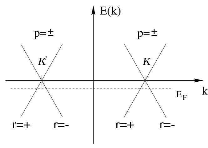
Figure 1: Schematic bandstructure of a metallic SWNT. A right- and left-moving branch ($r=\pm$) is found near each of the two Fermi points $k=\alpha k_{F}$ with $\alpha=\pm$, corresponding to $K$ and $K^{\prime}$, respectively. Right- and left-movers arise as linear combinations of the sublattices $p=\pm$. The Fermi energy (dashed line) is shifted away from neutrality by doping and/or external gates.

Besides SWNTs, LL effects have also been observed in the TDOS of multi-wall nanotubes (MWNTs) schoenen ; kim . MWNTs are composed of several concentrically arranged graphene shells, and under the assumption of ballistic transport, the only incomplete screening does not spoil the LL behavior mwnteg . On the other hand, transport in MWNTs has typical signatures of diffusive transport bachtold ; schoenen , and the theoretical situation must be regarded as unsettled at the moment. We shall therefore only discuss (metallic) SWNTs in this review.

The structure of the article is as follows. In Sec. 2, the theoretical description of a metallic SWNT in the ballistic limit is reviewed, where we focus on the low-energy regime $E<D$. We shall derive the scaling forms of the nonlinear $dI/dV$ characteristics for bulk or end tunneling into a nanotube, and point to various experimental setups that can detect correlation effects in the transport. We shall also briefly outline a recent suggestion for a spin-transport experiment that could allow for the experimental verification of spin-charge separation. In Sec. 3, the experimental evidence for LL behavior found so far is reviewed. Finally, in Sec. 4, we summarize and discuss some of the open problems that we are aware of.

2 Luttinger-liquid theory for nanotubes

2.1 Low-energy theory: General approach

The remarkable electronic properties of carbon nanotubes are due to the special bandstructure of the $\pi$ electrons in graphene. There are only two linearly independent Fermi points $\alpha\vec{K}$ with $\alpha=\pm$ instead of a continuous Fermi surface. Up to energy scales $E<D\approx 1$ eV, the dispersion relation around the Fermi points is, to a very good approximation, linear. Since the basis of the honeycomb lattice contains two atoms, there are two sublattices $p=\pm$, and hence two degenerate Bloch states

$$\varphi_{p\alpha}(\vec{r})=(2\pi R)^{-1/2}\exp(-i\alpha\vec{K}\vec{r})$$ (4)

at each Fermi point $\alpha=\pm$. Here $\vec{r}=(x,y)$ lives on the sublattice $p$ under consideration, and we have already anticipated the correct normalization for nanotubes. The Bloch functions are defined separately on each sublattice such that they vanish on the other. One can then expand the electron operator in terms of these Bloch functions. The resulting effective low-energy theory of graphene is the 2D massless Dirac hamiltonian. This result can also be derived in terms of $\vec{k}\cdot\vec{p}$ theory.

Wrapping the graphene sheet onto a cylinder then leads to the generic bandstructure of a metallic SWNT shown in Fig. 1. Writing the Fermi vector as $\vec{K}=(k_{F},p_{F})$, where the $x$-axis is taken along the tube direction and the circumferential variable is $0<y<2\pi R$, quantization of transverse motion now allows for a contribution $\propto\exp(imy/R)$ to the wavefunction. However, excitation of angular momentum states other than $m=0$ costs a huge energy of order $D\approx 1$ eV. In an effective low-energy theory, we may thus omit all transport bands except $m=0$ (assuming that the SWNT is not excessively doped). Evidently, the nanotube forms a 1D quantum wire with only two transport bands intersecting the Fermi energy. This strict one-dimensionality is fulfilled up to remarkably high energy scales (eV) here, in contrast to conventional 1D conductors. The electron operator for spin $\sigma=\pm$ is then written as

$$\Psi_{\sigma}(x,y)=\sum_{p\alpha}\varphi_{p\alpha}(x,y)\,\psi_{p\alpha\sigma}(x)\;,$$ (5)

which introduces slowly varying 1D fermion operators $\psi_{p\alpha\sigma}(x)$ that depend only on the $x$ coordinate. Neglecting Coulomb interactions for the moment, the hamiltonian is:

$$H_{0}=-\hbar v_{F}\sum_{p\alpha\sigma}p\int dx\;\psi_{p\alpha\sigma}^{\dagger}\partial_{x}\psi_{-p\alpha\sigma}\;.$$ (6)

Switching from the sublattice ($p=\pm$) description to the right- and left-movers ($r=\pm$) indicated in Fig. 1 implies two copies ($\alpha=\pm$) of massless 1D Dirac hamiltonians for each spin direction. Therefore a perfectly contacted and clean SWNT is expected to have the quantized conductance $G_{0}=4e^{2}/h$. Due to the difficulty of fabricating sufficiently good contacts, however, this value has not been experimentally observed so far. (We note that the conductance quantum $2e^{2}/h$ seen in recent MWNT experiments by Frank et al. frank is anomalous and does not correspond to the expected value of $G_{0}$.) Remarkably, other spatial oscillation periods than the standard wavelength $\lambda=\pi/k_{F}$ are possible. From Fig. 1 we observe that the wavelengths

$$\lambda=\pi/k_{F},\quad\pi/|q_{F}|,\quad\pi/(k_{F}\pm q_{F})$$ (7)

could occur, where the doping determines the wavevector $q_{F}\equiv E_{F}/\hbar v_{F}$. Which of the wavelengths (7) is ultimately realized sensitively depends on the interaction strength egger2 .

2.2 Electron-electron interactions

Let us now examine Coulomb interactions mediated by an arbitrary potential $U(\vec{r}-\vec{r}^{\prime})$. The detailed form of this potential will depend on properties of the substrate, nearby metallic gates, and the geometry of the setup. In the simplest case, bound electrons and the effects of an insulating substrate are described by a dielectric constant $\kappa$, and for an externally unscreened Coulomb interaction,

$$U(\vec{r}-\vec{r}^{\prime})=\frac{e^{2}/\kappa}{\sqrt{(x-x^{\prime})^{2}+4R^{2}\sin^{2}[(y-y^{\prime})/2R]+a_{z}^{2}}}\;,$$ (8)

where $a_{z}\approx a$ denotes the average distance between a $2p_{z}$ electron and the nucleus, i.e. the “thickness” of the graphene sheet. We neglect relativistic effects like retardation or spin-orbit coupling in the following. Electron-electron interactions are then described by the second-quantized hamiltonian

$$H_{I}=\frac{1}{2}\sum_{\sigma\sigma^{\prime}}\int d\vec{r}\int d\vec{r}^{\prime}\,\Psi^{\dagger}_{\sigma}(\vec{r})\Psi^{\dagger}_{\sigma^{\prime}}(\vec{r}^{\prime})U(\vec{r}-\vec{r}^{\prime})\Psi_{\sigma^{\prime}}(\vec{r}^{\prime})\Psi_{\sigma}(\vec{r})\;.$$ (9)

The interaction (9) can be reduced to a 1D form by inserting the expansion (5) for the electron field operator. The reason to do so is the large arsenal of theoretical methods readily available for 1D models. The result looks quite complicated at first sight:

$$H_{I}=\frac{1}{2}\sum_{pp^{\prime}\sigma\sigma^{\prime}}\sum_{\{\alpha_{i}\}}\int dxdx^{\prime}\;V^{pp^{\prime}}_{\{\alpha_{i}\}}(x-x^{\prime})\psi^{\dagger}_{p\alpha_{1}\sigma}(x)\psi^{\dagger}_{p^{\prime}\alpha_{2}\sigma^{\prime}}(x^{\prime})\psi_{p^{\prime}\alpha_{3}\sigma^{\prime}}(x^{\prime})\psi_{p\alpha_{4}\sigma}(x)\;,$$ (10)

with the 1D interaction potentials

$$V^{pp^{\prime}}_{\{\alpha_{i}\}}(x-x^{\prime})=\int dydy^{\prime}\varphi^{\ast}_{p\alpha_{1}}(\vec{r})\varphi^{\ast}_{p^{\prime}\alpha_{2}}(\vec{r}^{\prime})U(\vec{r}-\vec{r}^{\prime}+p\vec{d}\delta_{p,-p^{\prime}})\varphi_{p^{\prime}\alpha_{3}}(\vec{r}^{\prime})\varphi_{p\alpha_{4}}(\vec{r})\;.$$ (11)

These potentials only depend on $x-x^{\prime}$ and on the 1D fermion quantum numbers. For interactions involving different sublattices $p\neq p^{\prime}$ for $\vec{r}$ and $\vec{r}^{\prime}$ in Eq. (9), one needs to take into account the shift vector $\vec{d}$ between sublattices.

To simplify the resulting 1D interaction (10), we now exploit momentum conservation, assuming $E_{F}\neq 0$ so that Umklapp electron-electron scattering can be ignored. We then have “forward scattering” processes, where $\alpha_{1}=\alpha_{4}$ and $\alpha_{2}=\alpha_{3}$. In addition, “backscattering” processes may be important, where $\alpha_{1}=-\alpha_{2}=\alpha_{3}=-\alpha_{4}$. We first define the potential

$$V_{0}(x-x^{\prime})=\int_{0}^{2\pi R}\frac{dy}{2\pi R}\int_{0}^{2\pi R}\frac{dy^{\prime}}{2\pi R}\;U(\vec{r}-\vec{r}^{\prime})\;.$$ (12)

For the unscreened Coulomb interaction (8), this can be explicitly evaluated egger2 . From Eqs. (11) and (4), the forward scattering interaction potential reads $V_{0}(x)+\delta_{p,-p^{\prime}}\delta V_{p}(x)$, with

$$\delta V_{p}(x)=\int_{0}^{2\pi R}\frac{dydy^{\prime}}{(2\pi R)^{2}}[U(x+pd_{x},y-y^{\prime}+pd_{y})-U(x,y-y^{\prime})]\;,$$ (13)

which is only present if $\vec{r}$ and $\vec{r}^{\prime}$ are located on different sublattices. Thereby important information about the discrete nature of the graphite network is retained despite the low-energy continuum approximation. Since $V_{0}(x)$ treats both sublattices on equal footing, the resulting part of the forward scattering interactions couples only the total 1D electron densities,

$$H_{I}^{(0)}=\frac{1}{2}\int dxdx^{\prime}\,\rho(x)V_{0}(x-x^{\prime})\rho(x^{\prime})\;,$$ (14)

where the 1D density is $\rho=\sum_{p\alpha\sigma}\psi^{\dagger}_{p\alpha\sigma}\psi_{p\alpha\sigma}$. This part of the electron-electron interaction is the most important one and will be seen to imply LL behavior. Note that it is entirely due to the long-ranged  tail of the Coulomb interaction. All the remaining residual interactions come from short-ranged interaction processes, and since these are intrinsically averaged over the circumference of the tube, their amplitude is quite small and will (at worst) only cause exponentially small gaps. A related general discussion can be found in Ref. sawatzky .

For $|x|\gg a$, detailed analysis shows that $\delta V_{p}(x)=0$. However, for $|x|\leq a$, an additional term beyond Eq. (14) arises due to the hard core of the Coulomb interaction. At such small length scales, the difference between inter- and intra-sublattice interactions matters. To study this term, one should evaluate $\delta V_{p}(0)$ from microscopic considerations. One then finds the additional forward scattering contribution egger2

$$H^{(1)}_{I}=-f\int dx\sum_{p\alpha\alpha^{\prime}\sigma\sigma^{\prime}}\psi^{\dagger}_{p\alpha\sigma}\psi^{\dagger}_{-p\alpha^{\prime}\sigma^{\prime}}\psi_{-p\alpha^{\prime}\sigma^{\prime}}\psi_{p\alpha\sigma}\;,$$ (15)

where $f/a=\gamma_{f}e^{2}/R$. An estimate for armchair SWNTs yields $\gamma_{f}\approx 0.05$. Since these short-ranged interaction processes are averaged over the circumference of the tube, $f\propto 1/R$, and hence $f$ is very small. A similar reasoning applies to the backscattering contributions $\alpha_{1}=-\alpha_{2}=\alpha_{3}=-\alpha_{4}$ in Eq. (10). Because of a rapidly oscillating phase factor, the only non-vanishing contribution comes again from $|x-x^{\prime}|\leq a$, and we can effectively take a local interaction. Furthermore, only the part of the interaction which does not distinguish among the sublattices is relevant and leads to

$$H_{I}^{(2)}=b\int dx\sum_{pp^{\prime}\alpha\sigma\sigma^{\prime}}\psi^{\dagger}_{p\alpha\sigma}\psi^{\dagger}_{p^{\prime}-\alpha\sigma^{\prime}}\psi_{p^{\prime}\alpha\sigma^{\prime}}\psi_{p-\alpha\sigma}\;.$$ (16)

For the unscreened interaction (8), $b/a=\gamma_{b}e^{2}/R$ with $\gamma_{b}\approx\gamma_{f}$. For externally screened Coulomb interaction, one may have $b\gg f$.

Progress can then be made by employing the bosonization approach bosonization . For that purpose, one first needs to bring the non-interacting hamiltonian (6) into the standard form of the 1D Dirac model. This is accomplished by switching to right- and left-movers ($r=\pm$) which are linear combinations of the sublattice states $p=\pm$. In this representation, a bosonization formula generalizing Eq. (3) applies, now with four bosonic phase fields $\theta_{a}(x)$ and their canonical momenta $\Pi_{a}(x)$. The four channels are obtained from combining charge and spin degrees of freedom as well as symmetric and antisymmetric linear combinations of the two Fermi points, $a=c+,c-,s+,s-$. The bosonized expressions for $H_{0}$ and $H_{I}^{(0)}$ read

$$H_{0} = \sum_{a}\frac{\hbar v_{F}}{2}\int dx\left[\Pi_{a}^{2}+g^{-2}_{a}(\partial_{x}\theta_{a})^{2}\right]$$ (17)

$$H_{I}^{(0)} = \frac{2}{\pi}\int dxdx^{\prime}\;\partial_{x}\theta_{c+}(x)V_{0}(x-x^{\prime})\partial_{x^{\prime}}\theta_{c+}(x^{\prime})\;.$$ (18)

The bosonized form of $H_{I}^{(1,2)}$ egger leads to nonlinearities in the $\theta_{a}$ fields for $a\neq c+$. Although bosonization of Eq. (6) gives $g_{a}=1$ in Eq. (17) [see also Eq. (1)], interactions will renormalize these parameters. In particular, in the long-wavelength limit, $H_{I}^{(0)}$ can be incorporated into $H_{0}$ by putting

$$g_{c+}\equiv g=\left\{1+4\widetilde{V}_{0}(k\simeq 0)/\pi\hbar v_{F}\right\}^{-1/2}\leq 1\;,$$ (19)

while for all other channels, the coupling constant $f$ gives rise to the tiny renormalization $g_{a\neq c+}=1+f/\pi\hbar v_{F}\simeq 1$. The plasmon velocities of the four modes are $v_{a}=v_{F}/g_{a}$, and hence the charged $(c+)$ mode propagates with significantly higher velocity than the three neutral modes.

For the long-ranged interaction (8), the logarithmic singularity in $\widetilde{V}_{0}(k)$ requires the infrared cutoff $k=2\pi/L$ due to the finite length $L$ of the SWNT, resulting in:

$$g=\left\{1+\frac{8e^{2}}{\pi\kappa\hbar v_{F}}\ln(L/2\pi R)\right\}^{-1/2}\;.$$ (20)

Since $\hbar c/e^{2}\simeq 137$, we get with $v_{F}=8\times 10^{5}$ m/s the estimate $e^{2}/\hbar v=(e^{2}/\hbar c)(c/v)\approx 2.7$, and therefore $g$ is typically in the range $0.2$ to $0.3$. This estimate does only logarithmically depend on $L$ and $R$, and should then apply to basically all SWNTs studied at the moment (where $L/R\approx 10^{3}$). The LL parameter $g$ predicted by Eq. (20) can alternatively be written in the form

$$g=\left(1+\frac{2E_{c}}{\Delta}\right)^{-\frac{1}{2}}\;,$$ (21)

where $E_{c}$ is the charging energy and $\Delta$ the single-particle level spacing. For our experimental setup described in Sec. 3, the theoretically expected LL parameter is then estimated as $g_{\rm th}\approx 0.28$. The very small value of $g$ obtained here implies that an individual metallic SWNT on an insulating substrate is a strongly correlated system displaying very pronounced non-Fermi liquid effects.

It is clear from Eqs. (17) and (18) that for $f=b=0$, a SWNT constitutes a realization of the LL. We therefore have to address the effect of the nonlinear terms associated with the coupling constants $f$ and $b$. This can be done by means of the renormalization group approach. Together with a solution via Majorana refermionization, this route allows for the complete characterization of the non-Fermi-liquid ground state of a clean nanotube egger2 . From this analysis, we find that for temperatures above the exponentially small energy gap

$$k_{B}T_{b}=D\exp[-\pi\hbar v_{F}/\sqrt{2}b]$$ (22)

induced by electron-electron backscattering processes, the SWNT is adequately described by the LL model, and $H_{I}^{(1,2)}$ can effectively be neglected. A rough order-of-magnitude estimate is $T_{b}\approx 0.1$ mK. In the remainder, we focus on temperatures well above $T_{b}$.

2.3 Bulk and end tunneling: Scaling functions and exponents

Under typical experimental conditions, the contact between a SWNT and the attached (Fermi-liquid) leads is not perfect and the conductance is limited by electron tunneling into the SWNT, which in turn is governed by the TDOS. The TDOS exhibits power-law behavior and is strongly suppressed at low energy scales. The power-law exponent $\alpha>0$ depends on the geometry of the particular experiment: If one tunnels into the end of a SWNT, the exponent $\alpha_{\rm end}$ is generally larger than the bulk exponent $\alpha_{\rm bulk}$, since electrons can move in only one direction to accomodate the incoming additional electron. The end-tunneling exponent can be easily obtained from the open boundary bosonization technique bosonization . It follows that close to the boundary (taken at $x=0$), i.e. for $\max(x,x^{\prime})\ll v_{F}t$, the single-electron Greens function is of the form

$$\langle\Psi(x,t)\Psi^{\dagger}(x^{\prime},0)\rangle\propto t^{-(1/g+3)/4}\;.$$ (23)

The boundary scaling dimension of the electron field operator is therefore $\bar{\Delta}=\frac{1}{8g}+\frac{3}{8}$, as opposed to its bulk scaling dimension $\Delta=\frac{1}{16}\left(\frac{1}{g}+g\right)+\frac{3}{8}$. Making use of the text-book definition of the TDOS as the imaginary part of the electron Greens function, we find from Eq. (23) that the TDOS indeed vanishes as a power law with energy,

$$\rho(E)\propto(E/D)^{\alpha}\;,$$ (24)

where the exponent $\alpha$ is given by the end-tunneling exponent

$$\alpha_{\rm end}=2\bar{\Delta}-1=\left(\frac{1}{g}-1\right)/4\;.$$ (25)

Similarly one may derive the bulk-tunneling exponent:

$$\alpha_{\rm bulk}=2\Delta-1=\left(\frac{1}{g}+g-2\right)/8\;.$$ (26)

Since $\alpha>0$ for $g<1$, the TDOS vanishes as the energy scale $E$ approaches zero in both cases. For a Fermi liquid, however, both exponents are zero.

If transport is limited by tunneling through a weak contact from a metal electrode to the SWNT, the full nonlinear and temperature-dependent differential conductance $G(V,T)=dI/dV$ can be evaluated in closed form. If $V$ denotes the voltage drop across the weak link, one obtains

$$G(V,T)=AT^{\alpha}\cosh\left(\frac{eV}{2k_{B}T}\right)\left|\Gamma\left(\frac{1+\alpha}{2}+\frac{ieV}{2\pi k_{B}T}\right)\right|^{2}\;,$$ (27)

where $\Gamma$ denotes the gamma function and $A$ is a nonuniversal prefactor depending on details of the junction. The exponent $\alpha$ is either the end- or the bulk-tunneling exponent depending on the experimental geometry. If the leads are at finite temperature, the conductance is given by a convolution of Eq. (27) and the derivative of the Fermi function:

$$-df/dE=\frac{1}{4k_{B}T\cosh^{2}(eV/2k_{B}T)}\;.$$

Remarkably, the quantity $T^{-\alpha}G(V,T)$ should then be a universal  scaling function of the variable $eV/k_{B}T$ alone. This scaling is seen experimentally as discussed in Sec. 3.

2.4 Crossed nanotubes

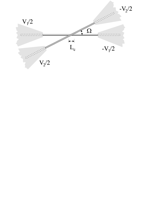
Figure 2: Crossed nanotube setup. By variation of the angle $\Omega$, the contact length $L_{c}$ can be changed. We consider a pointlike contact, $L_{c}\leq a$.

More spectacular correlation effects can be observed in more complicated geometries. The simplest example is provided by crossed nanotubes komnik which have recently been studied experimentally kim ; fuhrer . The geometry is shown in Figure 2, where we assume a pointlike contact of two clean metallic SWNTs characterized by the same $g$ parameter. External reservoirs can be incorporated by imposing Sommerfeld-like radiative boundary conditions egger96 close to the contacts (for simplicity, we sketch the theory for the spinless single-channel case). This approach offers a general and powerful route to studying multi-terminal Landauer-Büttiker geometries for correlated 1D systems. Applying the two-terminal voltage $V_{i}$ along conductor $i=1,2$, the boundary conditions read

$$\left(\frac{1}{g^{2}}\partial_{x}\pm\frac{1}{v_{F}}\partial_{t}\right)\langle\theta_{i}(x=\mp L/2,t)\rangle=\frac{eV_{i}}{\sqrt{\pi}\hbar v_{F}}\;.$$ (28)

These boundary conditions fix the average densities of injected particles. Outgoing particles are assumed to enter the reservoirs without reflection.

Let us now consider a point-like coupling at, say, $x=0$. Such a contact causes (at least) two different coupling mechanisms. First, there arises an electrostatic interaction $H_{c}^{(1)}\propto\rho_{1}(0)\rho_{2}(0)$. Bosonization shows that the only important part is

$$H_{c}^{(1)}=\lambda\cos[\sqrt{4\pi}\,\theta_{1}(0)]\cos[\sqrt{4\pi}\,\theta_{2}(0)]\;,$$ (29)

which becomes relevant for sufficiently strong interactions, $g<1/2$. The second potentially important process is single-electron tunneling from one conductor into the other. Notably, tunneling is always irrelevant for $g<1$, and (unless the contact is very good) can therefore be treated in perturbation theory. In other words, tunneling is expected to have only a very minor effect here, and we shall hence focus on the effect of $H_{c}^{(1)}$ specified in Eq. (29). Again, for $g>1/2$, this term can also be treated perturbatively, but for the interesting strong-interaction case $g<1/2$, qualitatively new features in the transport emerge.

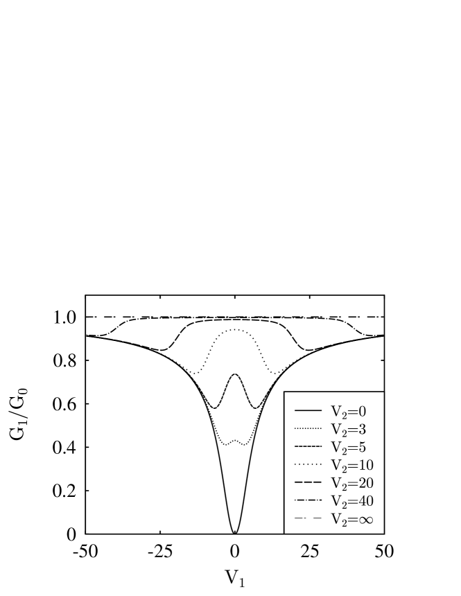
Figure 3: Conductance $G_{1}/G_{0}\equiv I_{1}/(e^{2}V_{1}/h)$ for $g=1/4,T=0$, and several values of the cross voltage $V_{2}$. The overall energy scale is set by the coupling $\lambda$.

To investigate this situation further, we switch to the linear combinations $\theta_{\pm}(x)=[\theta_{1}(x)\pm\theta_{2}(x)]/\sqrt{2}$, whence the hamiltonian decouples into the sum $H_{+}+H_{-}$ with

$$H_{\pm}=\frac{\hbar v_{F}}{2}\int dx\left\{\Pi_{\pm}^{2}+\frac{1}{g^{2}}(\partial_{x}\theta_{\pm})^{2}\right\}\pm(\lambda/2)\,\cos\left[\sqrt{8\pi}\,\theta_{\pm}(0)\right]\;.$$ (30)

Effective boundary conditions (28) for the fields $\theta_{\pm}$ are found by simply replacing $V_{1,2}\to(V_{1}\pm V_{2})/\sqrt{2}$. Therefore we are left with two completely decoupled systems, each of which is formally identical to the problem of an elastic potential scatterer embedded into a spinless LL with effectively doubled interaction strength parameter $g^{\prime}=2g$. The hamiltonian (30) has been discussed previously by Kane and Fisher kf , and the exact solution under the boundary condition (28) has recently been given by boundary conformal field theory methods saleur . This solution applies for arbitrary $g,T,V,$ and $\lambda$.

The conductance $G_{1}=I_{1}/(e^{2}V_{1}/h)$ for $g=1/4$ at zero temperature is plotted as a function of $V_{1}$ and $V_{2}$ in Fig. 3. Contrary to what is found in the uncorrelated case, $G_{1}$ is extremely sensitive to both $V_{1}$ and $V_{2}$ (in a Fermi liquid, $G_{1}$ is simply constant). For $V_{2}=0$, transport becomes fully suppressed for $V_{1}\to 0$, with a $g$-dependent perfect zero-bias anomaly (ZBA). Remarkably, there is a suppression of the current if $|V_{1}|=|V_{2}|$, which is observed as a “dip” in $G_{1}(V_{1})$ for fixed $V_{2}$. This effect can be rationalized in terms of a partial dynamical pinning of charge density waves in tube 1 due to commensurate charge density waves in tube 2. The consequence is that the ZBA dip at $V_{1}=0$ is turned into a peak by increasing the cross voltage $V_{2}$. The pronounced and nonlinear sensitivity of $G_{1}(V_{1},V_{2})$ to $V_{2}$ is a distinct fingerprint for LL behavior. Qualitatively, all these features have been observed in a very recent experiment by Kim et al. kim on crossed MWNTs.

2.5 Spin transport

The ultimate hallmark of a LL is electron fractionalization and spin-charge separation. So far no unambiguous experimental verification of spin-charge separation in a LL has been published, and carbon nanotubes might offer the possibility to do so. The standard approach via photoemission is clearly not suitable here since one should work on a single SWNT. Alternatively, a spin transport experiment will be described below that should reveal spin-charge separation in a clear manner balents . In such an experiment, one needs to measure the $I-V$ characteristics of a SWNT in weak contact to two ferromagnetic reservoirs, where the angle $\phi$ between the ferromagnet magnetization directions $\hat{m}_{1}$ and $\hat{m}_{2}$, i.e. $\cos\phi=\hat{m}_{1}\cdot\hat{m}_{2}$, can take an arbitrary value $0\leq\phi\leq\pi$. A corresponding experiment for $\phi=0,\pi$ has recently been performed for a MWNT FM-tube .

Spin transport has been studied in detail for Fermi liquids. For the proposed geometry of a metal connected to ferromagnetic leads via tunnel junctions, Brataas et al. brataas have computed the $\phi$-dependence of the current. Assuming identical junction and ferromagnet parameters, they obtain

$$\frac{I(\phi)}{I(0)}=1-P^{2}\frac{\tan^{2}(\phi/2)}{\tan^{2}(\phi/2)+Y}\;,$$ (31)

where the polarization $0\leq P\leq 1$ parametrizes the difference in the spin-dependent DOS of a ferromagnetic reservoir, and $Y\geq 1$ is related to the spin-mixing conductance brataas . The result (31) shows that for any $\phi>0$ the current will be suppressed due to the spin accumulation effect prinz . The maximum suppression, namely by a factor $1-P^{2}$, occurs for antiparallel magnetizations, $\phi=\pi$.

If one has spin-charge separation, detailed analysis balents shows that the current is still properly described by Eq. (31), though with two important differences. First, the current $I(0)$ for parallel magnetizations will carry the usual power-law suppression factor $(V/D)^{\alpha/2}$, where $\alpha>0$ is the bulk/end tunneling exponent. More importantly, the quantity $Y$ will now be $V$- and $T$-dependent, with a divergence as $V,T\to 0$ according to $Y\propto[{\rm max}(eV,k_{B}T)/D]^{-\alpha}$. Therefore the spin accumulation effect, i.e. the suppression of the current by changing $\phi$ away from zero, will be totally destroyed by spin-charge separation, except for $\phi=\pi$. This qualitative difference to a Fermi liquid should be easily detectable and can serve as a signature of spin-charge separation.

3 Experimental evidence for Luttinger liquid

In this section, we show first with electrostatic force microscopy (EFM) that metallic nanotubes are ballistic conductors, an important ingredient for the possible observation of LL behavior. When nanotubes are attached to metallic electrodes, EFM shows that a barrier is formed at the nanotube/metal interface. This fact is then exploited to observe LL behavior in nanotube devices via the TDOS. We show experimentally that the TDOS indeed exhibits power-law behavior in metallic SWNTs. This is observed by mesuring the tunneling conductance of nanotube/metal interfaces as a function of temperature and voltage.

3.1 Electrostatic Force Microscopy of electronic transport in carbon nanotubes

Samples are fabricated on a backgated substrate consisting of degenerately doped silicon capped with 1 $\mu$m SiO₂. SWNTs synthesized via laser ablation are ultrasonically suspended in dichloroethane, and the resulting suspension is placed on the substrate for approximately 15 seconds, then washed off with isopropanol. An array of structure, each consisting of two Cr/Au electrodes, is fabricated using electron beam lithography. Samples that have a measurable resistance between the electrodes are selected with a prober. An AFM is then used to choose samples that have only one nanotube rope between the electrodes. Objects whose height profile is consistent with single SWNTs (1-2 nm) are preferentially selected. An example of a SWNT rope contacted by two electrodes is shown in Fig. 4(a). Since the success of this contacting scheme works by chance, it is obvious that the yield is low. However, since a large array of structures can readily be fabricated, this scheme has turned out to be very convenient.

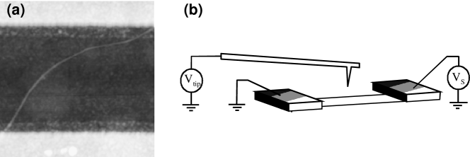
Figure 4: (a) Topographic AFM image of a 2.5 nm diameter bundle of SWNTs which is seen spanning between two gold electrodes. The separation between the electrodes is 1 $\mu$m. (b) Experimental setup for EFM. A conducting AFM cantilever is scanned above the device, which consists of a nanotube contacted by two gold electrodes. Adapted from Ref. bachtold .

We continue by reviewing the EFM technique efm2 which is used to directly probe the nature of conduction in SWNTs. An AFM tip with a voltage $V_{\rm tip}$ is scanned over a nanotube sample, see Fig. 4(b). The electrostatic force between the tip and the sample is given by

$$F=\frac{1}{2}\frac{dC}{dz}(V_{\rm tip}+\phi-V_{s})^{2}\;,$$ (32)

where $V_{s}$ is the voltage within the sample, $\phi$ is the work function difference between the tip and sample, and $C$ is the tip-sample capacitance. The tip is held at constant height above the surface by first making a line-scan of the topography of the surface using intermittent-contact AFM, and then making a second pass with the tip held at a fixed distance above the measured topographic features. In order to detect the electrostatic force, the cantilever is made to oscillate by an AC potential that is applied to the sample at the resonant frequency of the cantilever. This produces an AC force on the cantilever proportional to the local AC potential $V_{s}(w)$ beneath the tip:

$$F_{ac}(w)=\frac{dC}{dz}(V_{\rm tip}+\phi)\,V_{s}(w)\;.$$ (33)

The resulting oscillation amplitude is recorded using an external lock-in amplifier; the signal is proportional to $V_{s}(w)$. Calibration of this signal is made by applying a uniform $V_{s}(w)$ to the whole sample and measuring the response of the cantilever.

EFM yields a signal that is proportional to the local voltage within the nanotube circuit. However, the signal is also proportional to the derivative of the local capacitance. This will vary as the geometry changes, yielding e.g. different signals over a nanotube than over a contact at the same potential. However, $dC/dz$ does not vary appreciably as a function of distance along the nanotube. The measured signal should thus accurately reflect the local voltage within the nanotube.

3.2 Ballistic transport in metallic SWNTs

Next we discuss measurements of the device shown in Fig. 4. The resistance of this 2.5 nm diameter bundle is 40 k$\Omega$ and has no significant gate voltage dependence. We have also measured the current at large biases – the current saturates at 50 $\mu$A. This is in agreement with recent work by Yao, Kane and Dekker Yao where the current was observed to be limited to 25 $\mu$A per metallic nanotube due to optical or zone-boundary phonon scattering. We therefore conclude that the current is carried by 2 metallic SWNTs in the bundle.

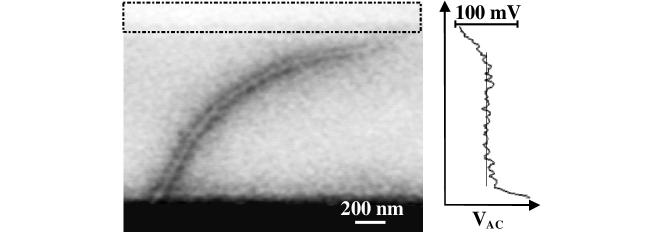
Figure 5: EFM image of the same bundle of SWNTs shown in Fig. 4. An AC potential of 100 mV is applied to the lower electrode. The upper electrode indicated by the box is grounded. The AC-EFM signal is flat along the length of the SWNT bundle, indicating that the potential drops occur at the contacts, and not along the bundle length. A trace of the potential as a function of vertical position in the image is also shown. Adapted from Ref. bachtold .

Figure 5 shows the EFM image of this SWNT bundle, as well as a line trace along the backbone of the bundle. The potential is flat over its length, indicating that within our measurement accuracy there is no measurable intrinsic resistance. Taking into account the finite measurement resolution, we estimate that $R_{i}$ of the bundle is at most 3 k$\Omega$. The contact resistances are measured to be approximately 28 k$\Omega$ and 12 k$\Omega$ for the upper and lower contacts, respectively. The conductance of the tube has been controlled to no change when the tip scans over it. The original data have a background signal due to stray capacitive coupling of the tip to the large metal electrodes. The image in Fig. 5 is shown with the background signal subtracted according to the procedure described in Ref. bachtold .

Using the four-terminal Landauer formula, $R=(h/4e^{2})(1-T_{i})/T_{i}$ per nanotube, where $T_{i}$ is the transmission coefficient for electrons along the length of the nanotube, we find that $T_{i}$ is larger than 0.5. This indicates that the majority of electrons are transported through the bundle with no scattering. Therefore transport is ballistic at room temperature over a length of $>1\mu$m. This confirms the theoretical predictions of very weak scattering in metallic SWNTs white ; anantram . This is also in agreement with previous low-temperature transport measurements which indicate that long metallic SWNTs may behave as single quantum dots tans ; bockrath2 , and room-temperature measurements of metallic SWNTs which sometimes exhibit low two-terminal resistance soh . The dominant portion of the overall resistance of 40 k$\Omega$ thus comes from the contacts, indicating that the transmission coefficients for entering and leaving the bundle are significantly less than one and the contacts are not ideal. As discussed in the next section, this fact can be exploited to observe LL behavior in nanotube devices via the tunneling density of states (TDOS).

3.3 Tunneling conductance

The fact that a metallic nanotube acts like a nearly perfect 1D conductor with very long mean free path makes it an ideal system to test the LL theory described in Sec. 2. Figure 6 shows the linear-response two-terminal conductance $G$ versus gate voltage $V_{g}$ for a metallic rope at different temperatures. At low temperatures, the conductance exhibits a series of Coulomb oscillations with a charging energy $E_{c}=1.9$ meV. For $k_{B}T>E_{c}$, i.e. $T>20K$, the Coulomb oscillations are nearly completely washed out, and the conductance is independent of gate voltage. A plot of the conductance vs. temperature in this regime is shown in the inset. The conductance drops steeply as the temperature is lowered, extrapolating to $G=0$ at $T=0$.

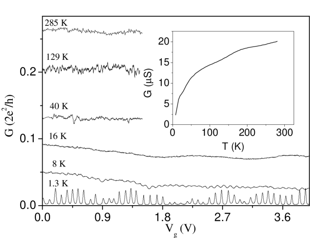
Figure 6: The two-terminal linear-reponse conductance as a function of gate voltage at a variety of temperatures. The inset shows the average conductance as a function of temperature. Adapted from Ref. bockrath .

Results for two samples are shown in Fig. 7(a), where the conductance as a function of temperature is plotted on a double-logarithmic scale (solid curves). Charging effects contribute to the measured characteristics, especially at lower temperatures, $k_{B}T<2E_{c}$. We therefore correct the $G(T)$ data for charging effects by dividing the measured conductance by the theoretically expected temperature dependence of $G$ in the Coulomb blockade model grabert . The dashed lines in Fig. 7(a) show the measured $G$ corrected in this manner as a function of temperature. Looking at the corrected data, we see that they have a finite slope, indicating an approximate power-law dependence upon temperature with exponents $\alpha=0.33$ and 0.38.

Figure 7(b) shows the measured differential conductance as a function of the applied bias $V$. The upper left inset to Fig. 7(b) shows $G=dI/dV$ versus $V$ at different temperatures, plotted on a double-logarithmic scale. At low bias, $dI/dV$ is proportional to a (temperature-dependent) constant. At high bias, $dI/dV$ increases with increasing $V$. The curves at different temperatures fall onto a single curve in the high-bias regime. Since this curve is roughly linear on the double-logarithmic plot, the differential conductance is well described by a power law, $dI/dV\propto V^{\alpha}$, where $\alpha=0.36$. At the lowest temperature $T=1.6$ K, this power-law behavior extends over two decades in the applied voltage $V$, namely from 1 mV up to 100 mV.

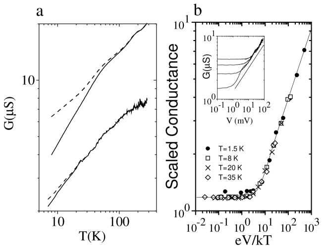
Figure 7: (a) Conductance plotted against temperature on a double-logarithmic scale for two samples. (b) The scaled differential conductance measured at different temperatures. Adapted from Ref. bockrath .

Let us next discuss possible origins of this behavior. The data demonstrates that tunneling into the rope has a significant dependence on energy that cannot be described by the Coulomb blockade model. One simple explanation for such behavior is that the transmission coefficients of tunnel barriers are strongly energy-dependent, with substantially increased transparency on the energy scale of the measurement. This would lead e.g. to activated transport over the barrier, $G\propto\exp(-\Delta/k_{B}T)$. However, the fact that the temperature dependence extrapolates to $G$ = 0 at $T$ = 0, see inset of Fig. 6, is inconsistent with this functional form. The origin of this behavior appears to originate rather from the TDOS of a LL which vanishes as a power law with energy, see Eq. (24). The assumption that the conductance is limited by tunneling between the metal electrodes and the LL directly leads to the power-law temperature dependence $G(T)\propto T^{\alpha}$ at small bias, $eV\ll k_{B}T$. Similarly, for $eV\gg k_{B}T$, LL theory predicts that $G(V)\propto V^{\alpha}$. The exponent $\alpha$ follows from the corresponding (bulk-tunneling, see below) exponent in the TDOS. We therefore obtain $\alpha_{\rm bulk}\approx 0.3$.

The devices used here were made in the following way. Electron beam lithography is first used to define leads, and ropes are deposited on top of the leads. Samples were selected that showed Coulomb blockade behavior at low temperatures with a single well-defined period, indicating the presence of a single dot. The charging energy of these samples indicates a dot with a size substantially larger than the spacing between the leads tans . Transport thus occurs by electrons tunneling into the middle (“bulk”) of the nanotubes. These devices are referred to as “bulk-contacted.” We can also use a second method, which was described in Sec. 3.1, where the contacts are applied over the top of the nanotube rope. From measurements of these devices in the Coulomb blockade regime bockrath2 , we conclude that the electrons are confined to the length of the rope between the leads. This implies that the leads cut the nanotubes into segments, and transport involves tunneling into the ends of the nanotubes. This type of device is referred to as “end-contacted.” For end-contacted devices, similar temperature and voltage dependences of the conductance $G(V,T)$ are observed. The obtained exponent $\alpha_{\rm end}\approx 0.6$ is significantly larger than $\alpha_{\rm bulk}\approx 0.3$, the exponent obtained for bulk-contacted devices.

The exponent of these power laws obviously depends on whether the electron tunnels into the end or the bulk of the LL. These exponents are related to the LL parameter $g$ by Eq. (25) and (26), respectively. Using the expected LL parameter $g_{\rm th}=0.28$, see Sec. 2.3, the expected exponents are $\alpha_{\rm end,th}=0.65$ and $\alpha_{\rm bulk,th}=0.24$. The approximate power-law behavior as a function of $T$ or $V$ observed in Fig. 7 follows the theory for tunneling into a LL. The predicted values of the exponents are in good agreement with the experimental values. Remarkably, power-law behavior in $T$ is observed up to 300 K, indicating that nanotubes are LLs even at room temperature.

LL theory makes an additional prediction for this system. Since the temperature and the voltage play an analogous role in the theory, the differential conductance for a single tunnel junction should obey the universal scaling form (27), together with a convolution of the derivative of the Fermi distribution, see Sec. 2.3. Hence it should be possible to collapse the data onto a single universal scaling curve. To do this, the measured nonlinear conductance $G(V,T)=dI/dV$ at each temperature was divided by $T^{\alpha}$ and plotted against $eV/k_{B}T$, as shown in the main body of Fig. 7(b). The data collapses well onto a universal curve. The solid line in Fig. 7(b) is the theoretical plot, see Ref. bockrath for details. The theory fits the scaled data quite well.

Recently, Yao et al. yao have reported on electrical transport measurements on SWNTs with intramolecular junctions. Two nanotubes are connected together by a kink, which acts as a tunnel barrier. In the case of a metal-metal junction, the conductance displays a power-law dependence on temperatures and voltage, consistent with tunneling between the ends of two LLs. The tunneling conductance $G$ across the junction is proportional to the product of the end-tunneling DOS on both sides. Therefore $G$ still varies as a power law of energy, but with an exponent twice as large, namely $\alpha_{\rm end-end}=2\alpha_{\rm end}$.

4 Discussion and open problems

In this review, we have discussed our recent observation of Luttinger liquid behavior in transport experiments on individual metallic carbon nanotubes, along with the detailed theoretical description of this non-Fermi liquid state. The situation in SWNTs seems rather clear by now, since the ballistic nature of transport can be unambiguously established. Nevertheless, several interesting open questions remain. One proposed experiment could probe spin-charge separation by measuring the $I-V$ characteristics of a SWNT in contact to two ferromagnetic reservoirs with continuously varying angle $\phi$ between the magnetization directions. Another interesting issue concerns the experimental observation of Friedel oscillations in nanotubes, i.e. density oscillations in the conduction electron density around impurities or the end of the tube. These density oscillations should decay with a slow interaction-dependent power law (slower than $1/x$), and, interestingly, the oscillation period can depend on the interaction strength egger2 . Furthermore, it is of importance to achieve a better understanding of conduction electron spin resonance (CESR) in SWNTs. Previous experimental attempts have not seen any ESR peak, and one of the proposed reasons for its absence involves electron-electron interactions forr . However, to the best of our knowledge, there are no theoretical investigations concerning CESR for Luttinger liquids including the gapless charge degrees of freedom. Finally, the phonon backscattering correction to the conductance arising for long SWNTs at high temperatures should involve an anomalous $T^{(1+g)/2}$ scaling komnik2 that remains to be seen experimentally.

Another line of research currently deals with multi-wall nanotubes which are known to exhibit diffusive transport. Nevertheless, the TDOS apparently shows very similar behaviors as in a SWNT, and superficially it appears that Luttinger liquid concepts also apply to MWNTs. The reason for this is presently unclear, and more theoretical and experimental studies will be needed to clarify the situation.

We acknowledges support by the DFG under the Gerhard-Hess program, by the DOE (Basic Energy Sciences, Materials Sciences Division, the sp2 Materials Initiative), and by DARPA (Moletronics Initiative).

References

- (1) S. Tomonaga: Prog. Theor. Phys. (Kyoto) 5, 544 (1950)
- (2) J.M. Luttinger: J. Math. Phys. (N.Y.) 4, 1154 (1963)
- (3) See, e.g., A.A. Abrikosov, L.P. Gorkov, I.E. Dzyaloshinskii: Methods of Quantum Field Theory in Statistical Physics (Dover, New York, 1963)
- (4) F.D.M. Haldane: J. Phys. C 14, 2585 (1981); Phys. Rev. Lett. 47, 1840 (1981)
- (5) See, e.g., A.O. Gogolin, A.A. Nersesyan, A.M. Tsvelik: Bosonization and Strongly Correlated Systems (Cambridge University Press, 1998), and J. v. Delft, H. Schoeller: Ann. Phys. (Leipzig) 7, 225 (1998)
- (6) M.P.A. Fisher, L.I. Glazman: in Mesoscopic Electron Transport, edited by L. Sohn et al. (Kluwer Academic Publishers, 1997)
- (7) K.V. Pham, M. Gabay, P. Lederer: Phys. Rev. B 61, 16397 (2000)
- (8) For a recent review, see J. Voit: Rep. Prog. Phys. 57, 977 (1995). See also: A. Schwartz, M. Dressel, G. Grüner, V. Vescoli, L. Degiorgi, T. Giamarchi: Phys. Rev. B 58, 1261 (1998)
- (9) S. Tarucha, T. Honda, T. Saku: Sol. State Comm. 94, 413 (1995)
- (10) O.M. Auslaender, A. Yacoby, R. de Picciotto, K.W. Baldwin, K.W. West: Phys. Rev. Lett. 84, 1764 (2000)
- (11) F.P. Milliken, C.P. Umbach, R.A. Webb: Sol. State Comm. 97, 309 (1996)
- (12) A.M. Chang, L.N. Pfeiffer, K.W. West: Phys. Rev. Lett. 77, 2538 (1996); M. Grayson, D.C. Tsui, L.N. Pfeiffer, K.W. West, A. Chang: Phys. Rev. Lett. 80, 1062 (1998)
- (13) R. Egger, A.O. Gogolin: Phys. Rev. Lett. 79, 5082 (1997); C.L. Kane, L. Balents, M.P.A. Fisher: Phys. Rev. Lett. 79, 5086 (1997)
- (14) R. Egger, A.O. Gogolin: Eur. Phys. J B 3, 281 (1998)
- (15) M. Bockrath, D.H. Cobden, J. Lu, A.G. Rinzler, R.E. Smalley, L. Balents, P.L. McEuen: Nature 397, 598 (1999)
- (16) Z. Yao, H.W.J. Postma, L. Balents, C. Dekker: Nature 402, 273 (1999)
- (17) C. Biagini, D.L. Maslov, M.Yu. Reizer, L.I. Glazman: preprint cond-mat/0006407
- (18) R. Mukhopadhyay, C.L. Kane, T.C. Lubensky: preprint cond-mat/0007039
- (19) S. Iijima: Nature 354, 56 (1991)
- (20) Special issue on Carbon Nanotubes in Physics World (June 2000), see especially articles by P. McEuen and by C. Schönenberger and L. Forró
- (21) C. Dekker: Physics Today (May 1999), p. 22
- (22) S.J. Tans, M.H. Devoret, H. Dai, A. Thess, R.E. Smalley, L.J. Geerligs, C. Dekker: Nature 386, 474 (1997); S.J. Tans, M.H. Devoret, R.J.A. Groeneveld, C. Dekker: Nature 394, 761 (1998)
- (23) M. Bockrath, D. Cobden, P. McEuen, N. G. Chopra, A. Zettl, A. Thess, R.E. Smalley: Science 275, 1922 (1997); D.H. Cobden, M. Bockrath, P.L. McEuen, A.G. Rinzler, R. Smalley: Phys. Rev. Lett. 81, 681 (1998)
- (24) A. Bachtold, M. Fuhrer, S. Plyasunov, M. Forero, E.H. Anderson, A. Zettl, P.L. McEuen: Phys. Rev. Lett. 84, 6082 (2000)
- (25) C.T. White, T.N. Todorov: Nature 393, 240 (1998)
- (26) A. Bachtold, C. Strunk, J.P. Salvetat, J.M. Bonard, L. Forró, T. Nussbaumer, C. Schönenberger: Nature 397, 673 (1999); C. Schönenberger, A. Bachtold, C. Strunk, J.P. Salvetat, L. Forró: Appl. Phys. A 69, 283 (1999)
- (27) J. Kim, K. Kang, J.O. Lee, K.H. Yoo, J.R. Kim, J.W. Park, H.M. So, J.J. Kim: preprint cond-mat/0005083
- (28) R. Egger: Phys. Rev. Lett. 83, 5547 (1999)
- (29) S. Frank, P. Poncharal, Z.L. Wang, W.A. de Heer: Science 280, 1744 (1998)
- (30) J. van den Brink, G.A. Sawatzky: Europhys. Lett. 50, 447 (2000)
- (31) A. Komnik, R. Egger: Phys. Rev. Lett. 80, 2881 (1998)
- (32) M.S. Fuhrer, J. Nygard, L. Shih, M. Forero, Y.G. Yoon, M.S.C. Mazzoni, H.J. Choi, J. Ihm, S.G. Louie, A. Zettl, P. McEuen: Science 288, 494 (2000)
- (33) R. Egger, H. Grabert: Phys. Rev. Lett. 77, 538 (1996); 80, 2255(E) (1998)
- (34) C.L. Kane, M.P.A. Fisher: Phys. Rev. B 46, 15233 (1992)
- (35) R. Egger, H. Grabert, A. Koutouza, H. Saleur, F. Siano: Phys. Rev. Lett. 84, 3682 (2000)
- (36) L. Balents, R. Egger: preprint cond-mat/0003038
- (37) K. Tsukagoshi, B.W. Alphenaar, H. Ago: Nature 401, 572 (1999)
- (38) A. Brataas, Yu. Nazarov, G.E.W. Bauer: Phys. Rev. Lett. 84, 2481 (2000)
- (39) G.A. Prinz: Physics Today 48(4), 58 (1995)
- (40) Y. Martin, D.W. Abraham, H.K. Wickramasinghe: Appl. Phys. Lett. 52, 1103 (1988); J.E. Stern et al.: Appl. Phys. Lett. 53, 2717 (1988); C. Schönenberger, S.F. Alvarado: Phys. Rev. Lett. 65, 3162 (1990)
- (41) Z. Yao, C.L. Kane, C. Dekker: Phys. Rev. Lett. 84, 2941 (2000)
- (42) M.P. Anantram, T.R. Govindan: Phys. Rev. B 58, 4882 (1998); T. Ando, T. Nakanishi, R. Saito: J. Phys. Soc. Jpn. (Japan) 67, 2857 (1998)
- (43) H.T. Soh, A.F. Morpurgo, J. Kong, C.M. Marcus, C.F. Quate, H. Dai: App. Phys. Lett. 75, 627 (1999)
- (44) H. Grabert, M.H. Devoret (eds.): Single Charge Tunneling, NATO-ASI Series B: Physics, vol. 294 (Plenum Press, New York, 1992)
- (45) L. Forró, private communcation
- (46) A. Komnik, R. Egger: in Electronic Properties of New Materials — Science and Technology of molecular nanostructures, AIP conference proceedings 486 (Melville, New York, 1999)