Dynamical Behaviour in the Nonlinear Rheology of Surfactant Solutions

Abstract

Several surfactant molecules self-assemble in solution to form long, flexible wormlike micelles which get entangled with each other, leading to viscoelastic gel phases. We discuss our recent work on the rheology of such a gel formed in the dilute aqueous solutions of a surfactant CTAT. In the linear rheology regime, the storage modulus $G^{\prime}(\omega)$ and loss modulus $G^{\prime\prime}(\omega)$ have been measured over a wide frequency range. In the nonlinear regime, the shear stress $\sigma$ shows a plateau as a function of the shear rate $\dot{\gamma}$ above a certain cutoff shear rate $\dot{\gamma}_{c}$. Under controlled shear rate conditions in the plateau regime, the shear stress and the first normal stress difference show oscillatory time-dependence. The analysis of the measured time series of shear stress and normal stress has been done using several methods incorporating state space reconstruction by embedding of time delay vectors.The analysis shows the existence of a finite correlation dimension and a positive Lyapunov exponent, unambiguously implying that the dynamics of the observed mechanical instability can be described by that of a dynamical system with a strange attractor of dimension varying from 2.4 to 2.9.

I Introduction

The amphiphilic nature of surfactant molecules results in their reversible self-assembling to form larger structures like spherical and cylindrical micelles, bilayers and vesicles. These supramolecular assemblies self-organise to form either long-range ordered liquid crystalline phases or short-range ordered isotropic liquid phases. Some examples of ordered phases are the nematic ordering of micellar discs or rods, the smectic A phase formed from the one-dimensional packing of infinite lamellae, cubic phases formed by finite-size spherical micelles and two-dimensional hexagonal crystals formed by infinite cylindrical micelles. In recent years, bicontinuous cubic phases have been observed in which a continuous bilayer or a monolayer forms a periodic, saddle-shaped, minimum energy surface. In isotropic phases, microemulsions and sponge phases can form. Another example is the formation of viscoelastic gels from the entanglement of very long and semiflexible cylindrical micelles with polymerlike behaviour. Interestingly, these micelles break and rejoin, giving rise to the name ’wormlike micelles’. The length distribution depends on the surfactant and the salt concentrations, temperature and the energy of scission of the micelles. The objective of this paper is to discuss our recent results on the nonlinear flow behaviour of such a system formed by the surfactant CTAT (cetyl trimethylammonium tosilate) in water. At very low concentrations, ($c<0.04$wt.%) and above the Kraft temperature of 23^∘C, CTAT molecules in water self-assemble to form spherical micelles exhibiting Newtonian flow. Above 0.9wt.%, CTAT forms giant wormlike micelles. The hexagonal phase is seen at a CTAT concentration of above 27wt.% sol1 ; sol2 .

In polymeric melts, stress relaxation occurs primarily by reptation dynamics (curvilinear diffusion of the polymeric chain along the contour of an imaginary tube enclosing the chain), as suggested by de Gennes deg , which defines a relaxation time $\tau_{rep}$. In systems of giant wormlike micelles, there is an additional contribution to the stress relaxation from the reversible scission (reversible breakage and recombination) of micelles, which occurs on a time scale $\tau_{b}$. If $\tau_{b}<<\tau_{rep}$, then stress relaxation in wormlike micelles occurs mainly by reversible scission and is described well by the Maxwell model which gives the response function G(t)=G${}_{o}exp{(-\frac{t}{\tau_{M}})}$, where G_o is the high frequency plateau modulus and $\tau_{M}=(\tau_{b}\tau_{rep})^{1/2}$ is the relaxation time. The physical picture of the single relaxation time is a kind of motional narrowing can ; cat .

The reptation reaction model of wormlike micelles, which gives the Maxwell model for the linear viscoelasticity, yields unusual nonlinear rheology observed in some viscoelastic gels (for example cetyl pyridinium chloride/ sodium salicylate) reh ; gran . The flow curve is characterised by a plateau in the shear stress versus shear rate curvereh , while the normal stress is found to increase linearly with shear rate reh ; spe . These features in the flow curve of giant wormlike micellar systems are associated with a flow instability of the shear banding type, where the sheared solution breaks up into bands of high and low viscosities supporting low and high shear rates, respectively spe . Flow birefringence mak and nuclear magnetic resonance velocity imaging mai have revealed the existence of banded flow in the shear stress plateau regime. An alternate hypothesis explains the plateau in the shear stress as due to an isotropic-nematic phase transition that occurs due to the application of high shear rates to the sample ber . Experiments on the transient rheology of CPyCl-NaCl after imposition of step shear rates, show overshoots, oscillations and long time sigmoidal kinetics in the shear stress $\sigma(t)$ ber . In our system of interest, CTAT 1.9wt.% in water at 25^∘C, we do not observe any overshoots in the stress relaxation on application of shear rates lying in the plateau region of the flow curve. However, we see that at high shear rates, the stress instead of decaying to a steady state, oscillates in time for a long time. We have analysed the time series of the viscoelastic and normal stresses obtained from these experiments and have demonstrated the existence of deterministic, chaotic dynamics in sheared solutions of CTAT. Oscillations in the stress relaxation of CTAT have also been observed by Soltero et al at a concentration of 5wt.% sol3 .

Chaotic time series data have often been observed in experiments on fluid dynamicsott . The Couette-Taylor flow in fluids and the Rayleigh-Benard convection in gases are two examples. Ananthakrishna et al ana have shown the existence of chaotic dynamics in the jerky flow (Portevin-Le Chatelier effect) of some metal alloys undergoing plastic deformation. These systems also exhibit nonmonotonic flow curves. Deterministic chaos represents the apparently irregular behaviour of dynamical systems that arises from strictly deterministic laws in the absence of any external stochasticity. Chaotic dynamics in physical systems is characterised by an exponentially sensitive dependence on initial conditions, as a result of which long-term predictability of the dynamics of these systems is impossible. Chaotic time series may be characterised by certain invariants, metric and dynamical, such as the various fractal dimensions, the largest Lyapunov exponent and the Kolmogorov entropy. A positive value of the largest Lyapunov exponent is a direct consequence of the sensitivity of the trajectories in phase space to small changes in the initial conditions. The fractal dimensions provide a measurement of the topology of the attractor on which all the trajectories asymptotically converge. Apart from describing the complexity of the attractor, they also provide a measure of the regularity of occurrence of the phase points on its surface abar .

In this paper, we will show the existence of a positive Lyapunov exponent and a finite correlation dimension in the observed time series of the stress relaxation of CTAT on application of step shear rates lying in the plateau region of the flow curve. Further, the magnitudes of the invariants are found to increase monotonically with shear rate, the control parameter in our experiments.

II Experimental Details

CTAT (purchased from Sigma Chemicals, India) samples were prepared by dissolving 1.9wt.% of powdered CTAT in distilled and deionised water. The samples were kept in an incubator at a temperature of 60^∘C for a week, and frequently shaken to facilitate homogenisation. The samples were then kept at the experimental temperature (25^∘C) for two days. The rheological properties of the CTAT thus prepared and equilibrated were measured using a Rheolyst AR-1000N ( T. A. Instruments, U. K.) stress-controlled rheometer with temperature control and software for shear rate control. The rheometer was also equipped with four strain gauge transducers at a distance of $R$ from the centre of the plate for the measurement of the normal force $F_{z}$. $F_{z}$ is related to the first normal stress difference Z by Z = ${\frac{2F_{z}}{\pi R^{2}}}$ mac . All the measurements reported in this paper were performed using a cone-and-plate geometry mac of diameter 4cm and cone angle 1^∘59”. In each flow experiment, the rheometer can collect upto a maximum of 1500 data points, with a time gap of 1s or more between acquisition of successive data points. Sample history effects were found to be important in CTAT and hence all experiments have been done on fresh samples from the same batch. Most of the experiments were performed at 25^∘C and a few at 35^∘C.

III Results

Fig. 1 shows the frequency response measurements at (a) 25^∘C and (b) 35^∘C. The linear regime was first ascertained by imposing stresses between 0.005 Pa to 2 Pa, oscillating at a frequency of 0.1 Hz, and finding the window of the applied stress values over which the elastic modulus G${}^{\prime}(\omega)$ and the viscous modulus G${}^{\prime\prime}(\omega)$ are constant. From this measurement, the oscillatory stress for the frequency response measurements at both the temperatures has been chosen to be 0.6 Pa.

Figure 1: Frequency response of CTAT 1.9wt.% at (a) 25^∘C and (b) 35^∘C, at an oscillatory stress of 0.6Pa. G${}^{\prime}(\omega)$ is indicated by solid circles and G${}^{\prime\prime}(\omega)$ by hollow squares. The solid and dashed lines show the fits to the Maxwell model for G${}^{\prime}(\omega)$ and G${}^{\prime\prime}(\omega)$, respectively.

In Figs. 1(a) and 1(b), the solid circles and the hollow squares represent G${}^{\prime}(\omega)$ and G${}^{\prime\prime}(\omega)$, respectively. The dominant relaxation time, estimated from the angular frequency at which G${}^{\prime}(\omega)$ and G${}^{\prime\prime}(\omega)$ are equal, is found to be 17s (1s) at 25^∘C (35^∘C). The solid (G${}^{\prime}(\omega)$) and dashed lines (G${}^{\prime\prime}(\omega)$) are the corresponding fits to the Maxwell model, given by $G^{\prime}(\omega)=\frac{G_{o}(\omega\tau_{M})^{2}}{1+(\omega\tau_{M})^{2}}$ and $G^{\prime\prime}(\omega)=\frac{G_{o}\omega\tau_{M}}{1+(\omega\tau_{M})^{2}}$. As mentioned before, for viscoelastic gels of wormlike micelles formed by the CTAC-NaSal,CPyCl-NaSal and CPySal-NaSal systems can ; gran , the Maxwell model works very well. However, for CTAT at 25^∘C, the fit of the data to the Maxwell model is rather poor. Interestingly, the fit is reasonably good for experiments done at 35^∘C. This may be due to the fact that the motional narrowing condition, $\tau_{b}<<\tau_{rep}$, is not satisfied at low temperatures.

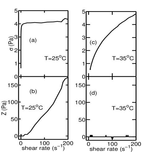
Figure 2: The metastable flow curves of CTAT 1.9wt.%, showing the shear stress and normal stresses, respectively, as a function of shear rate at 25^∘C ((a) and (b)) and 35^∘C ((c) and (d)).

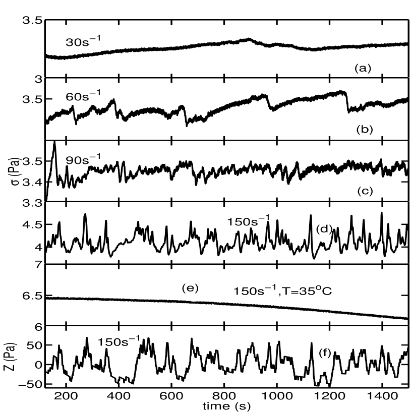
Figure 3: Shear stress relaxation measured in CTAT 1.9wt.% at 25^∘C on application of a step shear rate of (a) 30s^-1, (b) 60s^-1, (c) 90s^-1 and (d) 150s^-1. (e) shows the relaxation of shear stress at 35^∘C and $\dot{\gamma}$ = 150s^-1.(f) shows the relaxation of normal stress at 25^∘C on application of a shear rate of 150s^-1.

Fig 2 shows the viscoelastic stress and normal stress measurements when the stress was increased from 10 mPa to 4.7 Pa after allowing a time $\tau_{M}$ between acquisition of consecutive data points, and measuring the corresponding shear rate. These measurements give the metastable branches of the flow curve at 25^∘C (Fig. 2(a)) and 35^∘C (Fig. 2(c)). Figs. 2(b) and 2(d) show the measured normal stresses as a function of increasing shear rate at both the temperatures. At 25^∘C, the viscoelastic stress (2(a)) shows a crossover to a plateau, while the normal stress increases quadratically (2(b)) with increase in shear rate. The presence of a plateau in the viscoelastic stress at high shear rates is a signature of a mechanical instability, possibly of the shear banding type gran ; spe . We have ruled out the possibility of an isotropic-nematic phase transition on account of the very low volume fractions of CTAT used in our experiments. At 35^∘C, the viscoelastic stress does not show a plateau region and the normal stress is roughly zero, which implies the absence of instability in sheared solutions of wormlike micelles at higher temperatures por .

We have studied in great detail the relaxation of the viscoelastic stress on application of step shear rates lying in the plateau region of the flow curve. Fig. 3 (a)-(d) show the stress relaxation measured for 1500 seconds, after subjecting the sample to step shear rates of 30, 60, 90 and 150s^-1 (Figs. 3 (a)-(d)) at 25^∘C. The stress decays initially for t$\sim$100 seconds (not shown in Fig. 3), and then oscillates in time. This time-dependent behaviour of the stress becomes more pronounced at higher shear rates. Fig. 3(e) show the stress relaxation at 35^∘C on application of a step shear rate $\dot{\gamma}$ $=$ 150s^-1. The oscillations seen at 25^∘C at $\dot{\gamma}$=150s^-1 are found to disappear completely at 35^∘C, leading us to ascertain that the time-dependent oscillations observed in the stress at 25^∘C are a direct consequence of the mechanical instability in the system. The first normal stress difference Z, which is measured simultaneously with the viscoelastic stress $\sigma$ at $\dot{\gamma}$=150s^-1 also shows oscillations, as shown in Fig.3(f). In what follows, we describe how we have analysed the time-dependent data in $\sigma$ and Z to establish the presence of chaotic dynamics in the sheared CTAT solution. The time series analysis has been performed by using the method of state space construction by embedding time delay vectors ruel . Suppose {$\sigma_{j}=\sigma(j\Delta$ t), j=1,1500} denotes the time series in stress $\sigma$ on application of a step shear rate. $\Delta t=$ 1s is the time elapsed between collection of data points. In this method, we construst m-dimensional L-delay vectors given by {$\vec{X}_{i}=(\sigma_{i},\sigma_{i+L},\sigma_{i+2L},....,\sigma_{i+(m-1)L}$)}. {$\vec{X}_{i}$:i=1,2,…,N-(m-1)L} defines a trajectory in m-dimensional space due to the presence of a dynamics F$(\vec{X}_{i}):\vec{X}_{i}\rightarrow\vec{X}_{i+1}$. In doing so, it is crucial to choose the optimal embedding dimension $m_{o}$ and the optimal delay time $L_{o}$ properlytak . We have done this by analysing the local exponential divergence plots and the plots of $\gamma$ = $<ln(||\vec{X}_{i+k}-\vec{X}_{j+k}||/||\vec{X}_{i}-\vec{X}_{j}||)>$ versus L for the trajectories obtained by embedding the time series in m dimensions. Here $<..>$ denotes averaging over all $(i,j)$ pairs. Embedding the trajectories in higher dimensions leads to a reduction in the number of false neighbours as at m $<m_{o}$, we are not looking at the real dynamics, but at its projection. At m$>m_{o}$, the number of false neighbours is zero. The left panel of Fig 4 shows the local exponential divergence plots for $\dot{\gamma}$=150s^-1, where the abscissa is ln($||\vec{X}_{i}-\vec{X}_{j}||$) and the ordinate is ln($||\vec{X}_{i+k}-\vec{X}_{j+k}||/||\vec{X}_{i}-\vec{X}_{j}||$) for (L,m), where L= 1 and 5 and m=3 to 6. $||\vec{X}_{i}-\vec{X}_{j}||$ is the distance between the $i$th and $j$ th trajectories in m-dimensional space and is chosen to be smaller than a prescribed small distance r^⋆. $||\vec{X}_{i+k}-\vec{X}_{j+k}||$ is the Euclidian distance between $\vec{X}_{i}$ and $\vec{X}_{j}$ after k iterations of the dynamics F. For our analyses, we have chosen $r^{\star}$ to be equal to 4% of the maximum value of $||\vec{X}_{i}-\vec{X}_{j}||$. In all our calculations, k has been determined from the value of t at which the autocorrelation function $C_{L}(t)$ of the time series in $\sigma$ or Z falls to 1/e of its peak value. The plots are found to get increasingly compact at L=5 as m increases and there is no significant change as we go from m=5 to m=6. Hence we conclude that the optimal embedding dimension $m_{\circ}$ for our time series in $\sigma(t)$ at $\dot{\gamma}=$ 150s^-1 is 5.

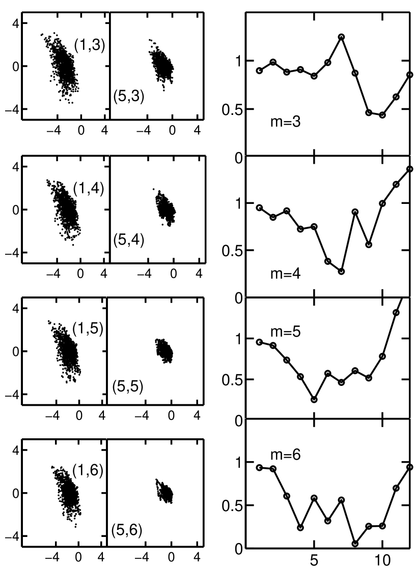
Figure 4: The left panel shows the local exponential divergence plots for typical values of m and L, marked as (L,m) for $\dot{\gamma}$=150s^-1. The abscissa is ln($||X_{i}-X_{j}||$) and the ordinate is ln($||X_{i+k}-X_{j+k}||/||X_{i}-X_{j}||$). The right panel shows the plots of $\gamma$ versus L at m=3 to 6, also for $\dot{\gamma}$=150s^-1. $\gamma$ has a minimum at m=5, L=5.

After obtaining a value of m from the local exponential divergence plots, we have plotted $\gamma$ versus L (right panel, Fig. 4) for m = 3 to 6. As m increases, $\gamma$ is found to decrease, and there is no significant change in the $\gamma$ versus L plot on changing m from m=$m_{\circ}$ (=5) to $m_{\circ+1}$ (=6). We see that $\gamma$ has a minimum at L = 5 for m = 5 and hence we have chosen the optimal delay time $L_{o}$ to be 5 and the optimal embedding dimension $m_{o}$ to be 5 for $\dot{\gamma}$=150s^-1.

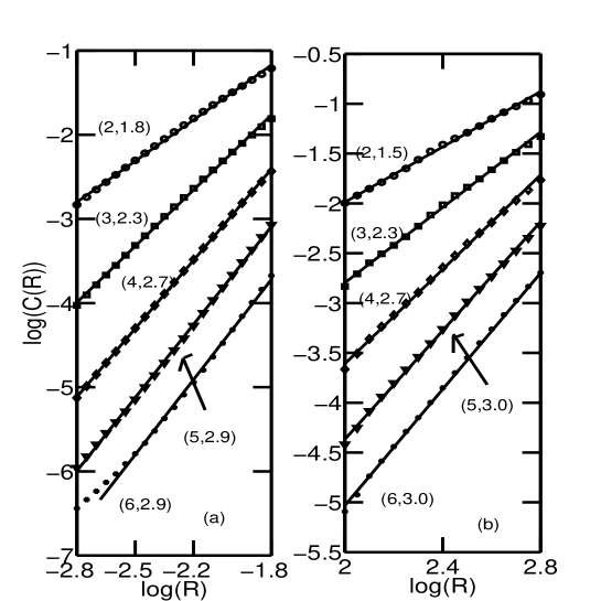
Figure 5: Calculation of the correlation dimensions $\nu$ from the time series corresponding to (a) shear stress $\sigma$ and (b) normal stress Z at 25^∘C and $\dot{\gamma}$=150s^-1, for m=2 to 6 (denoted by (m,$\nu$)). The values of $\nu$ calculated from the slopes of the plots of log(C(R)) versus log(R) are 2.9 for $\sigma$ and 3.0 for Z.

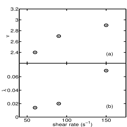
Figure 6: (a) The correlation dimension $\nu$ and (b) the Lyapunov exponent $\lambda$ as a function of the shear rate.

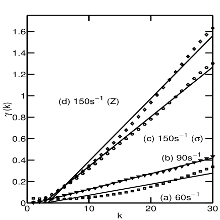
Figure 7: Plot of $\gamma$ versus k for the time series of the shear stresses $\sigma$ at (a) $\dot{\gamma}$=60 (m=5,L=11), (b)90 (m=5,L=9) and (c)150s^-1(m=5,L=5). (d) shows the same for the time series of the normal stress Z at $\dot{\gamma}$=150s^-1 (m=5,L=8). The Lyapunov exponents which can be estimated from the slope of the curves are found to be positive for all shear rates shown.

We have calculated the correlation dimensions $\nu$ of the attractors in state space on which the trajectories asymptotically lie by computing the correlation integral in m-dimensional space $C(R)={lim\atop N\rightarrow\infty}{1\over N^{2}}\sum_{i,j=1}^{N}H({R-||\vec{X}}_{i}-\vec{X}_{j}||)$ gra for m=2 to 6. In the expression for C(R), H(x) is the Heaviside function and $||\vec{X}_{i}-\vec{X}_{j}||$ is the distance between the pair of points ($i$,$j$) in the m-dimensional embedding space. The sum in the above expression gives the number of pairs of trajectories separated by a distance less than R. For small R’s, C(R) is known to scale as $C(R)\sim R^{\nu}$, where the correlation dimension $\nu$ gives useful information about the local structure of the attractor gra . The plot of C(R) versus R has a constant slope over a given range of R, which does not change on increasing m from m_∘ to m_∘+1 and is denoted by $\nu$. If $\nu<$ m, then the signal exhibits deterministic chaos. Fig. 5 shows the calculation of the correlation dimensions for the time series in viscoelastic stress $\sigma$ and normal stress Z at $\dot{\gamma}$=150s^-1. The slope of the C(R) versus R plot in the plateau region is found to saturate at m=5 in both cases yielding correlation dimensions $\nu$ of 2.9 and 3, respectively (Figs. 5(a)-(b)). The satisfaction of the condition $\nu<$m, and the value of $\nu>$2 points to the existence of deterministic chaotic dynamics gra in the stress relaxation of CTAT. We have also calculated the correlation dimensions of the attractors corresponding to the dynamics of stress relaxation at 60s^-1 and 90s^-1. The calculated values of $\nu$ in the two cases are 2.4 and 2.7 respectively, indicating the presence of chaotic dynamics at these shear rates. Fig 6(a) shows the calculated values of correlation dimensions $\nu$ as a function of the shear rate. $\nu$ is found to increase monotonically with the control parameter (shear rate in our case), similar to that observed in the weakly turbulent Couette-Taylor flow exhibited by orange oilswin , where the Rayleigh number was the control parameter.

A chaotic time series is characterised by a positive Lyapunov exponent, which describes the divergence of neighbouring trajectories in state space ott . We have calculated the largest Lyapunov exponents for the time series of the viscoelastic stresses at 60s^-1, 90s^-1 and 150s^-1 and the normal stress at 150s^-1 (Fig 7) using the method proposed by Gao and Zheng gao . This method requires the calculation of $\gamma(k)$ as a function of k, with $||\vec{X}_{i}-\vec{X}_{j}||\leq r^{\star}$ and $\vec{X}_{i}$ and $\vec{X}_{j}$ chosen such that $|j-i|\geq\omega$, where $\omega=(m-1)L$, to exclude tangential motion. A linear fit of $\gamma(k)$ versus k yields a positive slope S and nearly zero intercept, from which the Lyapunov exponent $\lambda$ has been extracted by using $\lambda=S/\Delta tln2$. $\lambda$ is found to increase monotonically with shear rate as shown in Figure 6(b).

IV Conclusions

The existence of a finite correlation dimension $\nu$ and a positive Lyapunov exponent $\lambda$ indicates the existence of deterministic chaos in the dynamics of stress relaxation in CTAT . This occurs only when the shear rates are high enough and lie in the plateau region of the flow curve. Since the volume fraction of CTAT in our experiment is very small, we rule out the possibility of an isotropic-nematic phase transition as the cause of the observed instabilities. We conclude that the chaotic dynamics is a natural consequence of the mechanical instability. The calculations described above predict an optimal embedding dimension $m_{o}$ of 5 for the description of the dynamics of the system. We have previously established the presence of chaotic dynamics in the stress relaxation in CTAT 1.35wt.%, when the sample was subjected to step shear rates lying in the plateau region of the flow curveran . However, at concentrations higher than 2.5wt.%, it is difficult to obtain a sufficiently long time series, as the large normal stresses that develop in the sample sol2 ; spe cause its expulsion from the rheometer.

In order to theoretically model the dynamical aspects of the observed phenomenon in viscoelastic gels, we need to set up space and time-dependent, coupled, nonlinear differential equations in at least 5 dynamical variables. One possible choice could be the Johnson-Segalman (J-S) equation joh which is the solution of the Navier-Stokes equation coupled to the continuity equation for isothermal, incompressible and viscoelastic fluids. The viscoelastic nature of the polymer is accounted for by writing the total stress as the sum of a Newtonian part and a deformation history-dependent viscoelastic part. This model yields a non monotonic flow curve and oscillations in the start-up stress in polymeric systemsmal . This model, however, has not been analysed to predict the chaotic time-dependence of the stresses that is seen in our experiments. We believe that the flow-concentration coupling and the dynamics of the mechanical interfaces between shear bands need to be incorporated in the J-S model. Further, the reversible breakdown and recombination of micelles also need to be considered. A model constructed by incorporating these additional features, which takes into account the nonlinear coupling between the relevant dynamical variables like shear and normal stress, shear rate and concentration profiles is likely to exhibit the chaotic behaviour that we observe.

V Acknowledgements

The authors thank Dr. Geetha Basappa for her participation in the initial part of the project and Dr. V. Kumaran, Dr. P. R. Nott and Dr. S. Ramaswamy for the use of the rheometer. AKS thanks the Board of Research in Nuclear Sciences and RB thanks CSIR, India for financial support

References

- (1) J.F.A.Soltero, J.E,Puig, O.Manero and P. C. Schulz, Langmuir, 11, 3337, (1995).
- (2) J. F. A. Soltero, J. E. Puig and O. Manero, Langmuir, 12, 2654, (1996).
- (3) P. G. de Gennes, J. Chem. Phys., 55, 572, (1971).
- (4) M. E. Cates and S. J. Candau, J. Phys. Condens Matter, 2 6869 (1990).
- (5) M. E. Cates, Macromolecules, 20, 2289, (1987).
- (6) H. Rehage and H. Hoffmann, Mol. Phys., 74, 933, (1991).
- (7) G.Grand, J. Arrault and M.E.Cates, J.Phys.II France, 7, 1071, (1997).
- (8) N. A. Spenley, M. E. Cates, and T. C. B. McLeish, Phys. Rev. Lett., 71, 939, (1993).
- (9) R. Makhloufi, J. P. Decruppe, A. Ait-Ali and R. Cressley, Europhys. Lett., 32, 253, (1995).
- (10) R. W. Mair and P. T. Callaghan, Europhys. Lett., 36, 719, 1996.
- (11) J. F. Berret , D. C. Roux and G. J. Porte, J. Phys. II, 4, 1261, (1994); J. F. Berret, Langmuir, 13, 2227, (1997).
- (12) J. F. A. Soltero, F. Batuista, J. E. Puig and O. Manero, Langmuir, 15, 1604 (1999).
- (13) E. Ott in Chaos in Dynamical Systems, Cambridge University Press, 1993.
- (14) S. J. Noronha, G. Ananthakrishna, L. Quaouire, C. Fressengeas and L. P. Kubin, Int. Jl. of Bifurcation and Chaos, 7, 2577, (1997).
- (15) H. D. I. Abarnel, R. Brown, J.J. Sidorowich and L. S. Tsimring, Rev. Mod. Phys.,65, 1331, (1993).
- (16) C. W. Macosko in Rheology Principles, Measurements and Applications, V. C. H. Publishers Inc., 1994, pp. 205-213.
- (17) G. Porte, J. F. Berret and J. L. Harden, J. Phys. II France, 7, 459, (1997).
- (18) J. P. Eckmann and D. Ruelle, Rev. Mod. Phys., 57, 617, (1985).
- (19) F. Takens in Dynamical Systems and Turbulence, Vol. 898 of Lecture Notes in Mathematics, edited by D. A. Rand and L. I. Young, Springer-Verlag, Berlin, 1981, p. 366.
- (20) P.Grassberger and I. Procaccia, Phys. Rev. Lett., 50, 346, (1983); P. Grassberger and I. Proccacia, Physica, 9D, 189, (1983).
- (21) A. Brandstater and H. L. Swinney, Phys. Rev. A, 35, 2207, (1987).
- (22) J. Gao and Z. Zheng,Phys. Rev. E 49, 3807, (1994).
- (23) Ranjini Bandyopadhyay, Geetha Basappa and A. K. Sood (submitted for publication).
- (24) M. W. Johnson and D. Segalman,J. Non-Newtonian Fluid Mech., 2, 255, (1977).
- (25) D. S. Malkus, J. A. Nohel and B. J. Plohr,J. Comp. Phys., 87, 464, (1990).