Theory of valence transitions
in ytterbium-based compounds

Abstract

The anomalous behavior of YbInCu₄ and similar compounds is modeled by the exact solution of the spin one-half Falicov-Kimball model in infinite dimensions. The valence-fluctuating transition is related to a metal-insulator transition caused by the Falicov-Kimball interaction, and triggered by the change in the f-occupancy.

I Introduction

The intermetallic compounds of the YbInCu₄ family exhibit an isostructural transition from high-temperature state with trivalent Yb ions in the $4f^{13}$ configuration to the low-temperature mixed-valent state with Yb ions fluctuating between $4f^{13}$ and $4f^{14}$ configurations [1]. The transition is particularly abrupt in high-quality stoichiometric YbInCu₄ samples [2] with a transition temperature equal to $T_{v}=42$ K at ambient pressure; the susceptibility and the resistivity drop at $T_{v}$ by more than one order of magnitude in cooling, while the volume expansion is small, $\Delta V/V\simeq 0.05$. The valence change inferred from $\Delta V/V$ by using the usual ionic radii of Yb³⁺ and Yb²⁺ is about $\Delta n_{f}\simeq 0.1$, which is consistent with the valence measurements by the $L_{III}$-edge absorption [1, 4]. The critical temperature depends strongly on external pressure, magnetic field, and alloying [5, 6]. A recent review of the experimental data is given in Ref. [7] and here we just recall the main points which motivate our choice of model.

The integer-valent phase ($T\geq T_{v}$) is characterized by a Curie-Weiss susceptibility [1, 6] with very small Curie-Weiss temperature $\Theta\ll T_{v}$. The Curie constant corresponds to the free moment of one magnetic f-hole in a $J=7/2$ spin-orbit state with $\mu_{eff}=4.53\mu_{B}$. The electrical resistance is large and has a small positive slope; it remains almost unchanged in magnetic fields up to 30 T [5]. In some systems, like Yb_1-xY_xInCu₄, the magnetoresistance is slightly negative, while in YbInCu₄ (or YbIn_1-xAg_xCu₄ for $x=0.15$) it is slightly positive [5]. The Hall constant is large and negative, indicating a small number of carriers [4, 8]. The thermoelectric power has a rather small slope which one finds in a semiconductor with a nearly symmetric density of states [9]. Recent data on the optical conductivity of YbInCu₄ [10] shows the absence of a Drude peak at high temperatures and a pronounced maximum of the optical spectral weight at about 1 eV. The high-temperature ESR data for Gd³⁺ embedded in YbInCu₄ resemble those found in integer-valence semi-metallic or insulator hosts [11]. Thus, the high-temperature phase indicates the presence of a well defined local moment but gives no signature of the Kondo effect. The overall behavior of the high-temperature phase is closer to that of a semi-metal or paramagnetic small-gap semiconductor than to a Kondo metal.

The mixed-valent phase ($T<T_{v}$) behaves like a Pauli paramagnet with moderately enhanced susceptibility and specific heat coefficient [6]. The electrical resistance and the Hall constant are one order of magnitude smaller than in the high-temperature phase [4, 8]. The thermoelectric power [9] has a very large slope typical of a valence fluctuator with large asymmetry in the density of states. The susceptibility, the resistivity and the Hall constant do not show any temperature dependence below $T_{v}$, which is also typical of valence fluctuators. The optical conductivity shows a major change with respect to the high-temperature shape. The peak around 1 eV is reduced, the Drude peak becomes fully developed, and an additional structure in the mid-infrared range appears quite suddenly below $T_{v}$ [10]. A large density of states at the chemical potential $\mu$ is indicated by the ESR data as well [12]. Thus, the transition at $T_{v}$ seems to be from a paramagnetic semimetal to a valence fluctuator.

In contrast to usual valence-fluctuators, which are quite insensitive to the magnetic field, the YbInCu₄ family of compounds also exhibit metamagnetic transitions when $T<T_{v}$. The Yb moment is fully restored at a critical field $H_{c}(T)$, with a Zeeman energy $\mu_{B}H_{c}$ comparable to the thermal energy $k_{B}T_{v}$. The metamagnetic transition defined by the magnetoresistance or the magnetization data [7] gives an H-T phase boundary $H_{c}(T)=H_{c}^{0}\sqrt{1-(T/T_{v})^{2}}$. The zero-temperature field $H_{c}^{0}$ is related to $T_{v}$ as $k_{B}T_{v}/\mu_{B}H_{c}^{0}=1.8$ [7].

To account for these features we need a model in which the non-magnetic, valence-fluctuating, metallic ground state can be destabilized by increasing temperature or magnetic field. Above the transition, we need a paramagnetic semiconductor with an average f-occupancy that is not changed much with respect to the ground state. The correct model for this system is a periodic Anderson model supplemented with a large Falicov-Kimball (FK) interaction term. The temperature or field induced transition suggests that one should place the narrow f-level just above the chemical potential $\mu$. The hybridization keeps the f-count finite below the transition, while large f-f correlations allow only the fluctuations between zero- and one-hole (magnetic) configurations. The low-temperature phase is close to the valence fluctuating fixed point and shows no Kondo effect. However, because of the Falicov-Kimball term, there is a critical f-occupation at which there is a transition into the high-temperature state with a large gap in the d- and f-excitation spectrum. The $n_{f}$ is driven to criticality either by temperature or magnetic field. In the high-temperature phase the hybridization can be neglected because the f-level width is already large due to thermal fluctuations, and quantum fluctuations are irrelevant. Unfortunately, the above model would be difficult to solve in a controlled way, and here we consider a simplified model in which the hybridization is neglected at all temperatures. This leads to a spin-degenerate Falicov-Kimball model which explains the collapse of the non-magnetic metallic phase at $T_{v}$ or $H_{c}$, and gives a good qualitative description of the high-temperature paramagnetic phase. However, the deficiency of the simplified model is that it yields a negligible f-count in the metallic phase and predicts a large change in the Yb valence at $T_{v}$ or $H_{c}$. It is clear that we can not obtain the valence fluctuating ground state and maintain the average f-occupancy below the transition without hybridization-induced quantum fluctuations. In what follows, we describe the model, explain the method of solution, and present results for static and dynamic correlation functions.

II Calculations

The Hamiltonian of the Falicov-Kimball model [13] consists of two types of electrons: conduction electrons (created or destroyed at site $i$ by $d_{i\sigma}^{\dagger}$ or $d_{i\sigma}$) and localized electrons (created or destroyed at site $i$ by $f_{i\sigma}^{\dagger}$ or $f_{i\sigma}$). The conduction electrons can hop between nearest-neighbor sites on the D-dimensional lattice, with a hopping matrix $-t_{ij}=-t^{*}/2\sqrt{D}$; we choose a scaling of the hopping matrix that yields a nontrivial limit in infinite-dimensions [14]. The $f$-electrons have a site energy $E_{f}$, and a chemical potential $\mu$ is employed to conserve the total number of electrons $n_{d\uparrow}+n_{d\downarrow}+n_{f\uparrow}+n_{f\downarrow}=n_{tot}$. The Coulomb repulsion $U_{ff}$ between two $f$-electrons is infinite and there is a Coulomb interaction $U$ between the $d$- and $f$-electrons that occupy the same lattice site. An external magnetic field $h$ couples to localized electrons with a Landé g-factor. The resulting Hamiltonian is [15, 16]

$$H=\sum_{ij,\sigma}(-t_{ij}-\mu\delta_{ij})d_{i\sigma}^{\dagger}d_{j\sigma}+\sum_{i,\sigma}(E_{f}-\mu)f_{i\sigma}^{\dagger}f_{i\sigma}$$ (1)

$$+U\sum_{i,\sigma\sigma^{\prime}}d_{i\sigma}^{\dagger}d_{i\sigma}f_{i\sigma^{\prime}}^{\dagger}f_{i\sigma^{\prime}}+U_{ff}\sum_{i,\sigma}f_{i\uparrow}^{\dagger}f_{i\uparrow}f_{i\downarrow}^{\dagger}f_{i\downarrow}$$ (2)

$$-\mu_{B}h\sum_{i,\sigma}\sigma(2d_{i\sigma}^{{\dagger}}d_{i\sigma}+gf_{i\sigma}^{{\dagger}}f_{i\sigma}).$$ (3)

The model can be solved in the infinite-dimensional limit by using the methods of Brandt-Mielsch [15]. We consider the hypercubic lattice with Gaussian density of states $\rho(\epsilon)=\exp[-\epsilon^{2}/t^{*2}]/\sqrt{\pi}t^{*}$, and take $t^{*}$ as the unit of energy ($t^{*}=1$). Our calculations are restricted to the homogeneous phase.

The local conduction-electron Green’s function satisfies Dyson’s equation

$$G^{\sigma}(z)=\int\frac{\rho(\epsilon)}{z+\mu-\Sigma^{\sigma}(z)-\epsilon}d\epsilon,$$ (4)

where $z$ is a complex variable and $\Sigma^{\sigma}$ is the local self energy which does not depend on momentum [14]. In infinite dimensions, $\Sigma^{\sigma}$ is defined by a sum of skeleton diagrams, which depend on the local d-propagator $G^{\sigma}$ but not on $t_{ij}$. The exact self-energy functional for the FK model is obtained by calculating the thermodynamic Green’s function [17] of an atomic system coupled to an external time-dependent field $\lambda^{\sigma}(\tau)$

$$G^{\sigma}_{\rm atom}(\tau)=-\frac{1}{\cal Z}{\rm Tr}_{df}\left<T_{\tau}e^{-\beta H_{\rm atom}}d_{\sigma}(\tau^{\prime})d_{\sigma}^{\dagger}(\tau)S(\lambda)\right>,$$ (5)

where the S-matrix for the $\lambda$-field is

$$S(\lambda)=T_{\tau}e^{-\int_{0}^{\beta}d\tau\int_{0}^{\beta}d\tau^{\prime}\lambda(\tau,\tau^{\prime})d_{\sigma}^{\dagger}(\tau)d_{\sigma}(\tau^{\prime})},$$ (6)

and $H_{\rm atom}$ is obtained from the Hamiltonian (3) by removing the hopping and keeping just a single lattice site. The exact solution for $G_{n}^{\sigma}[\{\lambda_{m}\}]$ at Matsubara frequency $i\omega_{n}=i\pi T(2n+1)$ is given by,

$$G_{n}^{\sigma}=\frac{w_{0}}{[G^{\sigma}_{0n}]^{-1}}+\frac{w_{1}}{[G^{\sigma}_{0n}]^{-1}-U},$$ (7)

where $w_{0}$ and $w_{1}$ are the f-occupation numbers ($w_{1}=1-w_{0}$, $w_{0}={\cal Z}_{0}/\cal Z$) and [15]

$${\cal Z}_{0}(\lambda,\mu)=2e^{\beta\mu/2}\prod_{n}\frac{1}{(i\omega_{n})G^{\uparrow}_{0n}}2e^{\beta\mu/2}\prod_{n}\frac{1}{(i\omega_{n})G^{\downarrow}_{0n}},$$ (8)

with

$${\cal Z}(\lambda,\mu)={\cal Z}_{0}(\lambda,\mu)+2e^{-\beta(E_{f}-\mu)}{\cal Z}_{0}(\lambda,\mu-U).$$ (9)

The bare Green’s function satisfies

$$G_{0n}^{\sigma}=\frac{1}{i\omega_{n}+\mu-\lambda^{\sigma}_{n}},$$ (10)

with $\lambda_{n}$ the Fourier transform of the external time-dependent field.

The self-energy functional $\Sigma_{n}^{\sigma}[G_{n}^{\sigma}]$ can now be obtained [15] by using the Dyson equation for the atomic propagator,

$$\Sigma_{n}^{\sigma}=[G_{0n}^{\sigma}]^{-1}-[G_{n}^{\sigma}]^{-1},$$ (11)

and eliminating $G_{0n}^{\sigma}[\{\lambda_{m}\}]$ from Eqs. (7) and (11). The mapping onto the lattice is achieved by adjusting $G_{0n}^{\sigma}$ in such a way that $G_{n}^{\sigma}[\{\lambda_{m}\}]$ satisfies the lattice Dyson equation (4).

The numerical implementation of the above procedure is as follows: We start with an initial guess for the self energy $\;\Sigma^{\sigma}\;$ and calculate the local propagator in (4). Using (11) we calculate the bare atomic propagator ${G_{0n}^{\sigma}}$ and find ${\cal Z}_{0}$ and $\cal Z$. Next we obtain $w_{0}$, $w_{1}$ and find $G_{n}^{\sigma}$ from (7). Using ${G_{0n}^{\sigma}}$ and $G_{n}^{\sigma}$, we compute the atomic self energy and iterate to the fixed point.

The iterations on the imaginary axis give static properties, like $n_{f}$, the f-magnetization $m_{f}(h,t)$, and the static spin and charge susceptibilities. Having found the f-electron filling $w_{1}$ at each temperature, we iterate Eqs. (4) to (11) on the real axis and obtain the retarded dynamical properties, like the spectral function, the resistivity, the magnetoresistance, and the optical conductivity. At the fixed point, the spectral properties of the atom perturbed by $\lambda$-field coincide with the local spectral properties of the lattice.

III Results and discussion

We studied the model for a total electron filling of 1.5 and for several values of $E_{f}$ and $U$. The main results can be summarized in the following way.

FIG. 1.: Number of the $f$-holes plotted versus $T/t^{*}$ for $U/t^{*}=4$. The $E_{f}/t^{*}$ increases from top to bottom, and is given by -0.7, -0.6, -0.5, and -0.2, respectively.

The occupancy of the f-holes at high temperatures is large and there is a huge magnetic degeneracy. The f-holes are energetically unfavorable but are maintained because of their large magnetic entropy. In Fig.(1) we show $n_{f}$ as a function of temperature, plotted for $U=4t^{*}$, and $E_{f}/t^{*}$ from -0.2 to -0.7. Below a certain temperature, which depends on $U$ and $E_{f}$, there is a rapid transition to the low-temperature phase. The transition becomes sharper and is pushed to lower temperatures as $E_{f}$ decreases at constant $U$. However, we restrict ourselves to continuous crossovers here, since the region with first-order transitions leads to numerical instabilities.

The uniform f-spin susceptibility is obtained by calculating the spin-spin correlation function [15, 16] and is given by $\chi(T)=Cn_{f}(T)/T$, where $C=g_{L}^{2}\mu_{B}^{2}J(J+1)/3k_{B}$ is the Curie constant.

FIG. 2.: Uniform static magnetic susceptibility of the $f$-holes plotted versus $T/t^{*}$ for $U/t^{*}=4$. The values of $E_{f}/t^{*}$ are the same as in Fig(1). The corresponding values of $T_{v}/t^{*}$ are estimated from the maximum of $\chi(T)$, and are given by 0.03, 0.08, 0.15, 0.35, respectively. The $T_{v}$ increases from top to bottom.

The $\chi(T)/C$ is shown in Fig. (2) for $U/t^{*}=4$ and for $E_{f}$ as quoted in Fig.(1). The $T_{v}$ is obtained from the maximum of the $\chi(T)/C$ and the values corresponding to various parameters used in this paper are quoted in the caption of Fig. (2). The high-temperature susceptibility follows an approximate Curie-Weiss law, but the Curie-Weiss parameters depend on the fitting interval.

The interacting density of states $\rho_{d}(\omega)$ for the conduction electrons is shown in Fig.(3) for $U/t^{*}=4$ and $E_{f}/t^{*}=-0.5$, and for several temperatures. (The energy is measured with respect to $\mu$.) The high-temperature DOS has a gap of the order of $U$, and the chemical potential is located within the gap. Below the transition $n_{f}$ is small, the correlation effects are reduced, and $\rho_{d}(\omega)$ assumes a nearly non-interacting shape, with large $\rho_{d}(\mu)$ and halfwidth $W\simeq t^{*}$.

The transport properties of the high-T phase are dominated by the presence of the gap, which leads to a small dc conductivity with a weak temperature dependence. The transport properties of the paramagnetic phase are unrelated to the spin-disorder Kondo scattering (there is no spin-spin scattering in the FK model). Below the transition the conductivity increases and assumes large metallic values.

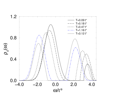
FIG. 3.: Interacting density of states plotted versus $\omega/t^{*}$ for $U/t^{*}=4$, $E_{f}/t^{*}=-0.5$ ($T_{v}/t^{*}=0.14$), and for various temperatures, as indicated in the figure.

The intraband optical conductivity $\sigma(\omega)$ is plotted in Fig.(4) as a function of frequency, for several temperatures. Above $T_{v}$, we observe a reduced Drude peak around $\omega=0$ and a pronounced high-frequency peak around $\omega\simeq U$. The shape of $\sigma(\omega)$ changes completely across $T_{v}$. Below $T_{v}$ the Drude peak is fully developed and there is no high-energy (intraband) structure. However, if the renormalized f-level is close to $\mu$, the interband d-f transition could lead to an additional mid-infrared peak. The ratio of the high-frequency peak in Fig(4) and the corresponding value of $T_{v}=0.15t^{*}$, is $U/T_{v}=26$. For the same value of U and $E_{f}=-0.7t^{*}$ ($T_{v}=0.03t^{*}$) we obtain $U/T_{v}=130$, while for $E_{f}=-0.75t^{*}$ ($T_{v}=0.02t^{*}$) we find $U/T_{v}\simeq 200$ (not shown).

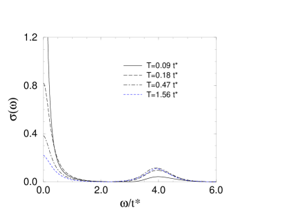
FIG. 4.: Optical conductivity plotted versus $\omega/t^{*}$ for various temperatures. The $U$, $E_{f}$, and $T_{v}$, are the same as in Fig.(3).

If we estimate the f-d correlation in YbInCu₄ from the 8000 $cm^{-1}$ peak in the optical conductivity data [10], we obtain the experimental value $U\simeq 1$ eV. Together with $T_{v}=42$ K [7] this gives the ratio $U/T_{v}\simeq 200$. If we take $U/t^{*}=4$ and adjust $E_{f}/t^{*}$ so as to bring the theoretical value of $T_{v}$ in agreement with the the thermodynamic and transport data on YbInCu₄, we get a high-frequency peak in $\sigma(\omega)$ at about 8000 $cm^{-1}$, 6000 $cm^{-1}$, and 1500 $cm^{-1}$, for $E_{f}=-0.75t^{*}$, $E_{f}=-0.7t^{*}$, and $E_{f}=-0.5t^{*}$, respectively.

FIG. 5.: The f-electron magnetization $m_{f}$ is plotted as a function of $h/t^{*}$ for various temperatures. The $U$, $E_{f}$, and $T_{v}$, are the same as in Fig.(3).

The f-electron magnetization $m_{f}(h)$ is plotted in Fig.(5) versus reduced magnetic field $h/t^{*}$, for several temperatures. Above the characteristic temperature $T_{v}^{*}\simeq T_{v}/2$, the $m_{f}(h)$ curves exhibit typical local moment behavior. Below $T_{v}^{*}$ we find a metamagnetic transition at a critical field $H_{c}$; the $m_{f}(h)$ is negligibly small below $H_{c}$ and the local moment is fully restored above $H_{c}$.

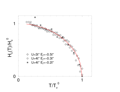
FIG. 6.: Normalized critical field is plotted as a function of reduced temperature $T/T_{v}^{*}$ for several values of $E_{f}/t^{*}$ and $U/t^{*}$. The full line represents $\sqrt{1-(T/T_{v}^{*})^{2}}$ and $T_{v}^{*}=T_{v}/2$.

Taking the inflection point of the $m_{f}(h)$ curves, calculated for several values of U and $E_{f}$, as an estimate of $H_{c}(T)$ we obtain the phase boundary which is shown in Fig.(6), together with the expression $H_{c}(T)/H_{c}^{0}=\sqrt{1-(T/T_{v}^{*})^{2}}$. Note, the $T_{v}^{*}$ values in Fig.(6) differ by more than an order of magnitude, while the ratio $k_{B}T_{v}^{*}/\mu_{B}H_{c}^{0}$ is only weakly parameter dependent.

FIG. 7.: Field-dependent resistivity plotted versus $h/t^{*}$. The different symbols correspond to different temperatures, as indicated in the figure. The $U$ and $E_{f}$ are the same as in Fig.(3).

The metamagnetic transition is also seen in the field-dependent electrical resistance $R(h,T)$ which is plotted in Fig.(7) as a function of $h/t^{*}$, for several temperatures. A substantial change in the $R(h,T)$ across $T_{v}^{*}$ or $H_{c}$ is clearly seen.

IV Summary

From the preceding discussion it is clear that Falicov-Kimball model captures the main features of the experimental data for YbInCu₄ and similar compounds. The temperature- and field-induced anomalies are related to a metal-insulator transition, which is caused by large FK interaction and triggered by the temperature- or the field-induced change in the f-occupancy. At high temperatures, we find a large gap in $\rho_{d}(\omega)$; we expect a similar gap in the f-electron spectrum as well. At low temperatures, both gaps are closed, and the renormalized f-level renormalizes down to the chemical potential.

Our calculations describe doped Yb systems with broad transitions but appear to be less successful for those compounds which show a first-order transition. The numerical curves can be made sharper (by adjusting the parameters) but they only become discontinuous in a narrow parameter range. The main difficulty with the FK model is that it predicts a substantial change in the f-occupancy across the transition and associates the loss of moment with the loss of f-holes. But in the real materials the loss of moment seems to be due to the valence fluctuations, rather than to the reduction of $n_{f}$. The description of the valence fluctuating ground state would require the hybridization and is beyond the scope of this work. The actual situation pertaining to Yb ions in the mixed-valence state might be quite complicated, since one would have to consider an extremely asymmetric limit of the Anderson model, in which the ground state is not Kondo-like, there is no Kondo resonance, and there is no single universal energy scale which is relevant at all temperatures [18].

We speculate that the periodic Anderson model with a large FK term will exhibit the same behavior as the FK model at high temperatures. Indeed, if the conduction band and the f-level are gapped, and the width of the f-level is large, then the effect of the hybridization can be accounted for by renormalizing the parameters of the FK model. On the other hand, if the low-temperature state of the full model is close to the valence-fluctuating fixed point with the conduction band and hybridized f-level close to the Fermi level, then the likely effect of the FK correlation is to renormalize the parameters of the Anderson model.

- [1] I. Felner and I. Novik., Phys. Rev. B 33, 617 (1986).
- [2] J.L. Sarrao et al., Physics B, 223&224, 366 (1996).
- [3] J. M. Lawrence et al., Phys. Rev. B,55, 14 467 (1997).
- [4] A. L. Cornelius et al., Phys. Rev. B,56, 7993 (1997).
- [5] C. D. Immer et al., Phys. Rev. B,56, 71 (1997).
- [6] J.L. Sarrao et al., Phys. Rev. B,58, 409 (1998)
- [7] J.L. Sarrao, Physica B, 259&261, 129 (1999)
- [8] E. Figueroa et al., Solid State Commun. 106, 347 (1998)
- [9] M. Očko, J. Sarrao, Z. Fisk, unpublished.
- [10] S. R. Garner et al., preprint (2000).
- [11] T. S. Altshuler et al., Z. Phys. B99, 57 (1995).
- [12] C. Rettori et al., Phys. Rev. B,55, 1016 (1997).
- [13] L. M. Falicov and J. C. Kimball, Phys. Rev. Lett. 22, 997 (1969).
- [14] W. Metzner and D. Vollhardt, Phys. Rev. Lett. 62, 324 (1989).
- [15] U. Brandt and C. Mielsch, Z.Phys. B 75, 365 (1989); U. Brandt and M. P. Urbanek, ibid. 89, 297 (1992).
- [16] J. Freericks and V. Zlatić, Phys. Rev. B 58, 322 (1998).
- [17] L.P. Kadanoff and G. Baym, Quantum Statistical Physics (W. A. Benjamin, Menlo Park, CA), 1962
- [18] H. B. Krishnamurti et al., Phys. Rev. B 21, 1044 (1980).