[

Transmission through quantum networks

Abstract

We propose a simple formalism to calculate the conductance of any quantum network made of one-dimensional quantum wires. We apply this method to analyze, for two periodic systems, the modulation of this conductance with respect to the magnetic field. We also study the influence of an elastic disorder on the periodicity of the AB oscillations, and we show that a recently proposed localization mechanism induced by the magnetic field resists to such a perturbation. Finally, we discuss the relevance of this approach for the understanding of a recent experiment on GaAs/GaAlAs networks.

]

It is well known that quantum transport exhibits deviations from classical transport, resulting in corrections to the classical addition rules of conductances or resistances. A spectacular example is the Aharonov-Bohm (AB) effect, where the conductance of a ring is a periodic function of the magnetic flux $\phi$ through its opening, with period $\phi_{0}=h/e$. Since the first observation of this effect in condensed matter[1], many papers have been devoted to the study of coherence effects in transport, especially in the ring geometry. A first approach uses the Landauer formalism in which the conductance is proportional to the transmission coefficient. In this framework, disorder effects have been considered in single-channel [2] and multi-channel rings [3]. On the other hand, the conductance of diffusive systems has been also extensively studied within the Kubo approach, where the weak-localization correction is related to the modulation by the magnetic field of the return probability of a diffusive particule [4]. Although being a transport property, this correction is a spectral quantity, since it is related to the spectrum of the diffusion equation, more precisely to its spectral determinant [5].

In this paper, we focus on the transmission properties of quantum networks, generalizing the original works of the 80’s [2, 6]. This work is motivated by recent conductance measurements of normal metallic networks etched on a 2D GaAs/GaAlAs electron gas [7]. Remarkably, for the particular ${\cal T}_{3}$ network shown in fig. 1, the magnetoresistance presents large $\phi_{0}$-periodic oscillations which are barely visible for a more conventional geometry like the square lattice. This is the first time that $\phi_{0}$ oscillations are observed in a macroscopic system where, in principle, ensemble average due to a finite coherence length is expected to destroy them.

The experimental study of the ${\cal T}_{3}$ network has been motivated by the recent prediction of a new type of magnetic field induced localization. Indeed, it has been shown, in a tight-binding approach, that when the flux $\phi$ per elementary plaquette equals $\phi_{0}/2$ (half-flux), the electron motion is completely confined inside the so-called AB cages [8] resulting from a subtle quantum interference effect. This surprising phenomenon has first been experimentally observed in superconducting (${\cal T}_{3}$) networks[9], where it was found that the critical current almost vanishes at $\phi=\phi_{0}/2$. The standard mapping between the Ginzburg-Landau theory and the tight-binding problem [10] actually allows one to relate this current to the energy band curvature, predicting a zero critical current at half-flux. However, it is interesting to know whether this localization effect still exists in normal metallic networks and if it could be at the origin of the oscillations discussed above [7].

The aim of this paper is threefold. Firstly, we provide a simple formalism allowing to calculate the transmission coefficient of any network made up of one-dimensional wires. Secondly, we concentrate on two regular structures, the square and the ${\cal T}_{3}$ networks and study the flux dependence of the transmission coefficient which is reminiscent of the butterfly-like structure of the tight-binding spectrum. We then consider the influence of elastic disorder that we model by a distribution of the wire lengths. We show that the ${\cal T}_{3}$ network exhibits $\phi_{0}$-periodic oscillations which are robust with respect to disorder and which are much larger than those observed in the square network. We also discuss the crossover from a ballistic (in the pure case) to a disorder dominated behaviour, revealed by the emergence of $\phi_{0}/2$-periodic oscillations reminiscent of the weak localization regime. This model gives a strong support to the interpretation of the above-mentionned experiment [7] in terms of the AB cages.

We consider a graph made up of $N$ nodes and connected to $N_{in}$ wires (also called channels) defining the input reservoir and to $N_{out}$ wires defining the outgoing reservoir (see fig. 1). In the Landauer approach, the two-terminal conductance is proportional to the total transmission coefficient defined by :

$$T=\sum_{i,j}|t_{ij}|^{2}\mbox{,}$$ (1)

where $i\in[1,N_{in}]$ denotes the $i^{th}$ input channel and $j\in[N-N_{out}+1,N]$ denotes the $j^{th}$ output channel. This coefficient is the sum of each individual transmission coefficient obtained by injecting a wavepacket in the $i^{th}$ channel. We emphasize that actually eq. (1) assumes that there is no phase relationship between the different input channels [11].

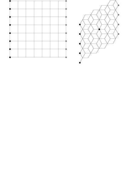
FIG. 1.: A piece of the ${\cal T}_{3}$ network (right) and of the square lattice (left). Black (respectively grey) dots represent the connections to the input (respectively output) channels. The central black dot is the input channel chosen for the bulk injection.

Let us consider an incoming wavefunction in the $i^{th}$ channel defined by :

$$\psi(x)=e^{-ikx}+r_{ii}e^{ikx}\mbox{,}$$ (2)

where $r_{ii}$ is the reflexion coefficient in this wire. We need to determine the transmission coefficient $t_{ij}$ giving the probability for the wave packet to outgo into the $j^{th}$ channel. Therefore, we first solve the Schrödinger equation on each bond whose extremities are denoted by $\alpha$ and $\beta$. The corresponding eigenfunctions are simply given by :

$$\psi_{\alpha\beta}(x)={e^{-i\gamma_{\alpha x}}\over\sin kl_{\alpha\beta}}\left[\psi_{\alpha}\sin k(l_{\alpha\beta}-x)+e^{i\gamma_{\alpha\beta}}\psi_{\beta}\sin kx\right]\mbox{,}$$ (3)

where $\gamma_{\alpha\beta}=(2\pi/\phi_{0})\int_{\alpha}^{\beta}{\bf A}.\mbox{d}{\bf l}$ is the circulation of the vector potential between $\alpha$ and $\beta$, $k$ is the wave vector related to the eigenenergy by : $E(k)=\hbar^{2}k^{2}/2m$, $x$ is the distance measured from the node $\alpha$ and $l_{\alpha\beta}$ is the length of the bond $(\alpha,\beta)$. The current conservation on each internal node of the network (not connected to reservoirs) is satisfied if :

$$M_{\alpha\alpha}\psi_{\alpha}+\sum_{\langle\alpha,\beta\rangle}M_{\alpha\beta}\psi_{\beta}=0\mbox{,}$$ (4)

where $M$ is a ($N\times N$) matrix whose elements are given by:

$$M_{\alpha\alpha}=\sum_{\langle\alpha,\beta\rangle}\cot kl_{\alpha\beta}\ \ ,\ \ M_{\alpha\beta}=-\frac{e^{i\gamma_{\alpha\beta}}}{\sin kl_{\alpha\beta}}\mbox{.}$$ (5)

The symbol $\langle\alpha,\beta\rangle$ indicates that the sums extend to all the nodes $\beta$ connected to the node $\alpha$. In addition, the off-diagonal element $M_{\alpha\beta}$ is non zero only if the nodes $\alpha$ and $\beta$ are connected by a bond. Consider now the case where the current is injected in the channel $i\in[1,N_{in}]$. The current conservation at this node writes :

$$M_{ii}\psi_{i}+\sum_{\langle i,\beta\rangle}M_{i\beta}\psi_{\beta}=i(1-r_{ii})\mbox{.}$$ (6)

For each node $j\in[N-N_{out}+1,N]$, one also has :

$$M_{jj}\psi_{j}+\sum_{\langle j,\beta\rangle}M_{j\beta}\psi_{\beta}=-it_{ij}\mbox{.}$$ (7)

Finally, for $i\in[1,N_{in}]$ and $j\in[N-N_{out}+1,N]$, the continuity of the wavefunction reads : $\psi_{i}=1+r_{ii}$ and $\psi_{j}=t_{ij}$. The equations (4,6,7) constitute a $(N\times N)$ linear system [12] from which $t_{ij}=\psi_{j}$ ($j\in[N-N_{out}+1,N]$) can be calculated. The total transmission coefficient is finally obtained from eq.(1) by considering the $N_{in}$ input channels.

We now apply this formalism to the case of regular networks where all the bonds have identical length $l$ so that the transmission coefficient $T(k,f)$ is a periodic function of the wave vector $k$ with period $2\pi/l$ and a periodic function of the reduced flux $f=\phi/\phi_{0}$ with period $1$. In principle, the $k$-dependence of the transmission coefficient can be probed experimentally, if the wave vector $k$ is well defined, i.e. if the energy of injected electrons is well controlled. Several factors like finite temperature or finite bias contribute to broaden this energy. This can be taken into account by giving a finite width $\Delta k$ to the Fermi wave vector of the incoming wave packet. For example, in ref. [14] the conductance of a single ring was measured and it was found that the phase of the AB oscillations could be varied by tuning the gate voltage, and thus the Fermi energy. One may therefore conclude that the width $\Delta k$ is smaller than the period $2\pi/l$. These oscillations are very well described by a Landauer single-channel formalism, assuming that the ring is assymetric, i.e. the two arms have a different length [2, 14].

For a given $k$, the flux dependence of $T(k,f)$ has a rich structure which is reminiscent of the complexity of the associated tight-binding spectrum. Here, for simplicity, we have chosen to average the transmission coefficient over a period $k\in[0,2\pi/l]$. The flux dependence of the average transmission $\langle T(k,f)\rangle_{k}$ is shown in fig. 2 for the square and ${\cal T}_{3}$ networks. One clearly observes a few peaks in the transmission for particular values of the reduced flux : $f=1/2,1/3$ for the square lattice and $f=1/3,1/6$ for the ${\cal T}_{3}$ lattice. One can simply understand this structure by invoking the extended nature of the corresponding eigenstates that are Bloch waves with a spatial period proportional to the denominator of $f$ [13]. Due to the existence of the AB cages, the transmission coefficient is minimum at $f=1/2$ for the ${\cal T}_{3}$ network but, surprisingly, it is not exactly zero. This is due to the existence of dispersive edges states [15] that are able to carry current even for $f=1/2$. Therefore, $T$ converges toward a finite value for the ${\cal T}_{3}$ network when the system size (and $N_{in}$) increases, whereas $T\sim N_{in}$ in the square lattice. However, when one injects current in the bulk of the sample, the transmission completely vanishes for this flux. (see inset fig. 2). This study shows that the cage effect, originally predicted in a tight-binding model, also arises in a ${\cal T}_{3}$ network made up of one-dimensional ballistic wires.

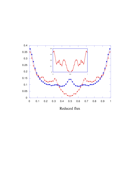
FIG. 2.: Averaged transmission coefficient $\langle T(k,f)\rangle_{k}/N_{in}$ as a function of the reduced flux for a $(8\times 8)$ square lattice (square) and a piece of the ${\cal T}_{3}$ network (triangle) with 75 sites. Input and output channels are connected as displayed in fig. 1. Inset : Averaged transmission coefficient for the ${\cal T}_{3}$ network with one input channel at the center of the network.

We now consider the case of disordered networks, the motivation being to see whether the cage phenomenon persists in such a situation. Disorder can be introduced in several ways (randomly distributed pointlike scatterers, or more generally, random elastic scattering matrix along the bonds). Here, in order to simulate random phase shifts on each bond, we consider a geometrical disorder defined by a random modulation of the wire lengths while keeping the same connectivity. Denoting by $\Delta l$ the amplitude of the length fluctuations, the relevant dimensionless parameter to characterize the strength of the disorder is the quantity $k\Delta l$ and thus explicitly depends on the energy. Note that the incommensurability between the different lengths breaks the periodicity of $T$ with respect to $k$. This type of disorder also provides a distribution of areas of width $2l\Delta l$ so that the oscillations are expected to disappear after about $l/\Delta l$ periods. In the following, we will focus on situations where $\Delta l/l\ll 1$ and $k\>l\gg 1$ so that the case $k\Delta l\sim 1$ may be reached without a sizeable dispersion of the areas. Thus, we will not modify the bond lengths in the phase factor $e^{i\gamma_{\alpha\beta}}$ and the periodicity with respect to the reduced flux will be conserved.

For a given realisation of disorder, $T(k,f)$ exhibits a $\phi_{0}$-periodic complex structure which is a signature of the interference pattern through the network. In particular, the transmission extremely sensitive to $k$. However, experimentally, there is always a finite phase coherence length $L_{\varphi}$. Therefore, a two-dimensional network of typical linear size $L$ must be considered as a set of $(L/L_{\varphi})^{2}$ regions without phase relationship. This provides a natural averaging mechanism over disorder realisations. Thus, we have chosen to study the disorder averaged transmission coefficient $\langle T(k,f)\rangle_{dis.}$ whose variations versus the reduced flux are displayed in fig. 3 for fixed $k$ and disorder strength. It is clearly seen that for the square network, the periodicity of $\langle T(k,f)\rangle_{dis.}$ with respect to the magnetic flux is no longer $\phi_{0}$ but $\phi_{0}/2$. The $\phi_{0}$-periodic oscillations have been washed out since they do not have a given phase. By contrast, the $\phi_{0}/2$-periodic oscillations are still present since they are related to phase coherent pairs of time-reversed trajectories according to the weak-localization picture. For the ${\cal T}_{3}$ network, the transmission coefficient remains $\phi_{0}$-periodic with a large amplitude. This strongly suggests that the cage effect (which locks the phase of the oscillations) survives for this strength of disorder.

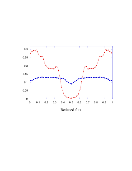
FIG. 3.: Transmission coefficient $\langle T(k,f)\rangle_{dis.}/N_{in}$ averaged over 50 configurations of disorder for $kl=\pi/3$ and $k\Delta l=1.47$ as a function of the reduced flux.

For a finer analysis, it is interesting to compute the discrete Fourier transform of $T$ defined by :

$$\tilde{T}(k,\omega)={1\over n}\sum_{j=0}^{n-1}T(k,j/n)e^{i2\pi\omega j/n}\mbox{,}\>\>\>\omega\in[0,n-1]\mbox{,}$$ (8)

where $n$ is the number of sampled values of $f$. Figure 4 displays $\langle|\tilde{T}(k,1)|\rangle_{dis.}$ as a function of the disorder strength $k\Delta l$ for different values of $k$. It shows that, when disorder is increased, $\langle|\tilde{T}(k,1)|\rangle_{dis.}$ persists much longer for the ${\cal T}_{3}$ network than for the square network. We are thus led to conclude that the cage effect is robust with respect to disorder. Note that for weak disorder, $\langle|\tilde{T}(k,1)|\rangle_{dis.}$ depends on $k$ but this dependence vanishes for $k\Delta l\gtrsim 2$. We strongly believe that this result explains why a $\phi_{0}$-periodic conductance is observed experimentally for the ${\cal T}_{3}$ network while it is not for the square lattice [7].

The behaviour of $\langle|\tilde{T}(k,2)|\rangle_{dis.}$ is shown in fig. 5. It is interesting to see that this harmonic becomes quickly dominant for both networks and remains constant for $k\Delta l\gtrsim 2$. The value of this constant depends on the system size and converges to zero for the infinite lattice. Nevertheless, we leave the precise analysis of this scaling for further studies.

Finally, it should be stressed that, experimentally, $\langle|\tilde{T}(k,2)|\rangle_{dis.}$ is further reduced by a factor $e^{-2L/L_{\varphi}}$ due to a finite coherence length $L_{\varphi}$, while the $\phi_{0}$ contribution is only reduced by a factor $e^{-L/L_{\varphi}}$, $L$ being the perimeter of an elementary plaquette [4].

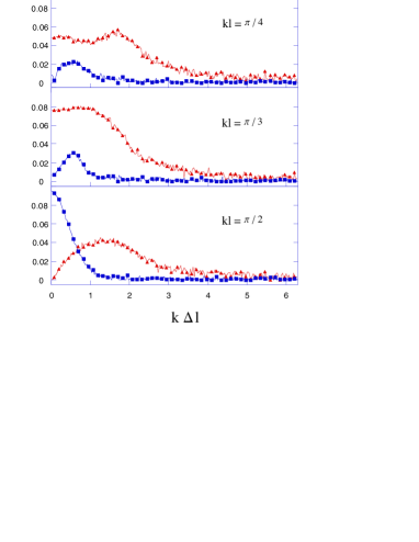
FIG. 4.: Variation of $\langle|\tilde{T}(k,1)|\rangle_{dis.}/N_{in}$ versus disorder for different values of $k$ after averaging over 50 configurations.

In conclusion, we have used a simple and general formalism to calculate the transmission coefficient of any network made up of single-channel quantum wires. This coefficient can be simply expressed in terms of a connectivity-like matrix. We have used this formalism to study the AB cage phenomenon in the ${\cal T}_{3}$ network and we have shown that this effect is robust to a moderate amount of elastic disorder. As a consequence, the AB oscillations with period $\phi_{0}$ persist in the infinite ${\cal T}_{3}$ networks whereas they vanish in the square lattice.

We acknowledge H. Bouchiat, P. Butaud, R. Deblock, G. Faini, D. Mailly, R. Mosseri, C. Naud and B. Reulet for useful discussions.

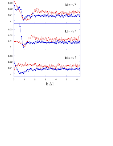
FIG. 5.: Amplitude of the second harmonic $\langle|\tilde{T}(k,2)|\rangle_{dis.}/N_{in}$ versus disorder for different values of $k$ after averaging over 50 configurations.

REFERENCES

- [1] S. Washburn and R. Webb, Adv. Phys. 35, 375 (1986).
- [2] M. Büttiker, Y. Imry and M. Ya. Azbel, Phys. Rev. A 30, 1982 (1984).
- [3] M. Büttiker, Y. Imry, R. Landauer and S. Pinhas, Phys. Rev. B 31, 6207 (1985).
- [4] A.G. Aronov and Yu.V. Sharvin, Rev. Mod. Phys. 59, 755 (1987).
- [5] M. Pascaud and G. Montambaux, Phys. Rev. Lett. 82, 4512 (1999).
- [6] B. Douçot and R. Rammal, J. Physique (Paris) 48, 941 (1987).
- [7] C. Naud, G. Faini, D. Mailly and B. Etienne preprint : cond-mat/006400.
- [8] J. Vidal, R. Mosseri and B. Douçot, Phys. Rev. Lett. 81, 5888 (1998).
- [9] C.C. Abilio et al., Phys. Rev. Lett. 83, 5102 (1999).
- [10] P.G. de Gennes, C.R. Acad. Sci. Ser. B 292, 9 and 279 (1981), S. Alexander, Phys. Rev. B 27, 1541 (1983).
- [11] Y. Imry, Introduction to mesoscopic physics, Oxford University Press (1997).
- [12] T. Kottos and U. Smilansky, Ann. Phys. 274, 76 (1999).
- [13] Note that since the peak resolution is set by the size of the sample, one would observe higher order peaks for much bigger systems.
- [14] S. Pedersen et al., Phys. Rev. B 61, 5457 (2000).
- [15] J. Vidal et al., in preparation.