Statistics of energy levels and zero temperature dynamics for deterministic spin models with glassy behaviour

Abstract

We consider the zero-temperature dynamics for the infinite-range, non translation invariant one-dimensional spin model introduced by Marinari, Parisi and Ritort to generate glassy behaviour out of a deterministic interaction. It is shown that there can be a large number of metatastable (i.e., one-flip stable) states with very small overlap with the ground state but very close in energy to it, and that their total number increases exponentially with the size of the system.

1 Introduction

A main issue in glassy systems is the analogy between glass-forming liquids and discontinuous spin-glasses, first pointed out in the pioneering works by Kirkpatrick, Thirumalai and Wolynes [KTW]. In both cases the thermodynamical properties can be indeed related to the dynamical evolution in an energy landscape. In liquid theory one can define the notion of inherent structures [SW] (local minima of the potential energy, each one surronded by its attraction basin or valley) and configurational entropy, i.e. the logarithm of the number of these minima divided by the number of particles in the system. Then the low-temperature dynamical evolution can be described as a superposition of an intra-basin “fast” motion and a “slow” crossing of energy barriers. If the temperature of the system is small enough, namely less than the Mode Coupling critical temperature $T_{MC}$, the system gets trapped in one of the basins. Since the number of energy minima diverges exponentially with the size of the system, a thermodynamic transition can be associated with an entropy crisis: the Kauzmann temperature $T_{K}$ of the glassy transition corresponds to the vanishing of the configurational entropy. We refer the reader to [MP] for an overview on equilibrium thermodynamics of glasses.

Consider now the class of discontinuous spin glasses, i.e. the mean-field models involving a random $p$-spin interaction. Also these models show a dynamical transition at a temperature $T_{D}$ (corresponding to $T_{MC}$) where dynamical ergodicity breaks down; a thermodynamic entropy-driven transition takes place at a lower temperature $T_{1RSB}$ (corresponding to $T_{K}$), at which replica symmetry breaks down with a “one step” pattern. Here the local minima of the free energy correspond to the solutions of the mean field TAP equations. Anyway at temperature $T=0$ metastable states with respect to any dynamics reduce to $1$-spin-flip stable states.

The main gap in the analogy between structural glasses and discontinuous spin-glasses is that in the latter models, unlike the former, the couplings between spins are quenched random variables. A significant, recent step in filling this gap has been made by the introduction of the deterministic, i.e. non-random, spin models which show a dynamical phase transition with a discontinuous order parameter and an equilibrium phase transition at a lower temperature associated with the vanishing of the high-temperature entropy [MPR, BM, BDGU, NM, PP]. It is the high degree of frustation among the couplings, not the disorder, to generate a huge number of metastable states and thus the glassy behaviour. The discovery of these models proved that disorder is not necessary to reproduce a complex free energy landscape.

Metastables states in infinite-range disordered spin-glasses have been extensively studied, both in the SK model where the number of $1$-spin-flip stable states scales like $\exp(0.1992N)$ [TE, BrM, DGGO, MPV], $N$ being the size of the system (number of spins in the one-dimensional case), and in $p$-spin interaction spin-glasses [OF].

Here we deal with the same question in deterministic models. By probabilistic arguments we will obtain, for the models introduced in [MPR], a lower bound on the number of $1$-spin-flip stable states, which increases exponentially with the size of the system. Hence this deterministic model exhibits the main feature of glassy behaviour.

The paper is organized as follows: in Section 2 we review the basic properties of the model we consider, the sine model of [MPR], a deterministic, one dimensional chain of $N$ spins with long-range oscillating interaction. In Section 3 we study the limiting distribution of the rescaled energy density, showing that it gets $\delta$-distributed in the thermodynamic limit. This property, which holds for the Curie-Weiss case, is an indication of the mean-field nature of the model. In Section 4 we deal with the state space of the system, computing explicitly (for $N$ prime analytically, for other values of $N$ numerically) the distribution of the energy levels by flipping one spin at a time; among other things we show that there can be a large number of states with almost zero overlap with the ground state but very close in energy to it. Finally, in Section 5 we derive the main result of the paper, that is a lower exponential bound for the number of metastable states at temperature $T=0$. Acknowledgments: M. D.E. contributed to this paper during his visit to the School of Mathematics of the Georgia Institute of Technology, whose support and excellent working conditions he gratefully acknowledges.

C. G. wants to thank the Department of Physics of Brown University, where part of this work was performed, for the kind hospitality during his visit under the exchange program between the Bologna and Brown Universities .

2 Orthogonal interaction matrices and the sine model

The basic setup is a probability space $(\Sigma_{N},{\cal{F}}_{N},{\rm P}\,_{N})$. The sample space $\Sigma_{N}$ is the configuration space, i.e. $\Sigma_{N}=\{-1,1\}^{N}$ whose elements are the sequences $\sigma=(\sigma_{1},\cdots,\sigma_{N})$ with $\sigma_{i}=\pm 1$; ${\cal{F}}_{N}$ is the finite algebra with $2^{2^{N}}$ elements, and the a priori (or infinite-temperature) probability measure ${\rm P}\,_{N}$ is given by

$${\rm P}\,_{N}(C)={1\over 2^{N}}\sum_{\sigma\in C}1.$$ (2.1)

The Hamiltonian is the function on $\Sigma_{N}$ defined as

$$H(\sigma)=-{1\over 2}\sum_{xy}J_{xy}\,\sigma_{x}\,\sigma_{y}=-{1\over 2}<J\sigma,\sigma>$$ (2.2)

where $J=(J_{xy})$ is a symmetric real orthogonal $N\times N$ matrix given from the outset. Although many of the results presented here will hold for a generic symmetric orthogonal matrix (e.g. of the form $J=OLO^{T}$ with $L$ a diagonal matrix whose elements are $\pm 1$ and $O$ a generic orthogonal matrix chosen at random w.r.t. the Haar measure on the orthogonal group) in what follows we shall examine the following particular example known as the sine model:

$$J_{xy}={2\over\sqrt{2N+1}}\sin\left({2\pi xy\over 2N+1}\right).$$ (2.3)

which satisfies (we assume $N$ odd)

$$J\,J^{T}={\rm Id}\quad\hbox{and}\quad\sum_{x=1}^{N}J_{xx}=\sum_{x=1}^{N}J_{xx}^{2}=1.$$ (2.4)

This model has been introduced by Marinari, Parisi and Ritort as a deterministic system with high frustration (competiting interactions with different signs and strengths) able to reproduce the complex thermodynamical behaviour typical of spin glasses [MPR]. It has been investigated analytically in the high-temperature regime, (through an high-temperature expansion), and numerically also in the low-temperature phase (using Montecarlo annealing). The analytical study revealed the existence of a static phase transition at a temperature $T_{S}=0.065$ where the high-temperature entropy vanishes, while evidence of the existence of a higher temperature $T_{D}=0.134$ where the system undergoes a dynamical transition of second order (i.e. with a jump in the specific heat) with a discontinuous order parameter has been put forward by numerical analysis. It has also been shown, using the replica formalism, that most of the thermodynamical properties of this model are the same as those of a generic symmetric orthogonal matrix (the static transition corresponding to RSB while the dynamical transition being given by the so-called “marginality condition”).

3 The limiting distribution of the rescaled energy levels.

The knowledge of the eigenvalues of $J$ imposes simple bounds on the energy of any spin configuration. Indeed a state vector $\sigma$ can be decomposed into his projections on the various orthogonal eigenspaces relatives to different eigenvalues. Here, due to orthogonality, the possible eigenvalues are $+1,-1$ so that

$$-\frac{N}{2}\leq H(\sigma)\leq\frac{N}{2}.$$ (3.5)

Let us consider the rescaled and shifted Hamiltonian (representing the energy per site, or energy density of the model, plus the ‘zero point’ energy $1/2$)

$$h(\sigma)={H(\sigma)\over N}+{1\over 2}$$ (3.6)

which takes values in $[0,1]$. We shall show that in the limit $N\to\infty$ the energy density $h$ gets $\delta$-distributed at $x=1/2$. We point out that this property can be immediately proved for the Curie-Weiss model, thus indicating a mean field behaviour of the present model in the thermodynamic limit. To this end consider the partition function $Z_{N}$ at inverse temperature $\beta$:

$$Z_{N}(\beta)=\sum_{\sigma\in\Sigma_{N}}\exp{(-\beta H(\sigma))}=2^{N}\,{\rm E}\,_{N}(e^{-\beta H}),$$ (3.7)

where ${\rm E}\,_{N}$ denotes the expectation wrt ${\rm P}\,_{N}$, and note that the characteristic function of $h$ can be written as

$${\rm E}\,_{N}(e^{-\lambda h})=e^{-\lambda/2}\,{Z_{N}(\lambda/N)\over 2^{N}}.$$ (3.8)

This expression will prove useful to compute the limiting expression of the characteristic function of the energy density $h$ without knowing the expression of all its moments. To see this, we first decouple the spins as follows: let $B$ be an orthogonal matrix such that $B^{T}JB=D$ with $D={\rm diag}\,(d_{1},\dots,d_{N})$. Since ${\rm det}\,J\neq 0$ we have $d_{i}\neq 0$, $i=1,\dots,N$, and ${\rm det}\,J^{-1}=\prod_{i}d_{i}^{-1}$. Let $u\in I\!\!R^{N}$ be such that $\sigma=Bu$. We have $<J\sigma,\sigma>=<Bu,JBu>=<u,Du>$, and thus

$$\exp({\lambda\over 2N}<J\sigma,\sigma>) = \prod_{i=1}^{N}\exp({\lambda\over 2N}d_{i}u_{i}^{2})$$

$$= \prod_{i=1}^{N}{1\over\sqrt{2\pi}}\int_{-\infty}^{\infty}\exp\left(-{x_{i}^{2}\over 2}+\sqrt{{\lambda d_{i}\over N}}\,\,u_{i}x_{i}\right)dx_{i}$$

$$= {1\over(2\pi)^{N/2}}\int_{I\!\!R^{N}}\exp\left(-{1\over 2}<x,x>+\sqrt{{\lambda\over N}}\,\,<u,D^{1/2}x>\right)\,dx$$

$$= {{\rm det}\,J^{-{1\over 2}}\over(2\pi\lambda)^{N/2}}\int_{I\!\!R^{N}}\exp\left(-{1\over 2\lambda}<y,J^{-1}y>+\,<\sigma,{y\over\sqrt{N}}>\right)\,dy,$$

which, together with (2.2), (3.7) and (3.8) yields

$${\rm E}\,_{N}(e^{-\lambda h})=e^{-{\lambda/2}}\,{{\rm det}\,J^{-{1\over 2}}\over(2\pi\lambda)^{N/2}}\int_{I\!\!R^{N}}\exp\biggl{(}-{1\over 2\lambda}<y,J^{-1}y>+\sum_{i}\log\cosh{y_{i}\over\sqrt{N}}\biggr{)}\,dy$$

(As usual, the square roots appearing in the above formulas are only apparently ill defined: they disappear in the expansion because it contains only the even terms). The above integral can be evaluated by means of standard high-temperature expansion techniques which turn out to be considerably simpler if one assumes that $\sum_{i}J_{ii}=0$ (see [PP]). As we have already noted, this assumption amounts to fix at zero the mean value of the energy. Also, the division by $N$ of the argument of the partition function leads to a convergence domain which is increasing as $N$ itself. In this way, the asymptotic expression (for $N\to\infty$) of ${\rm E}\,_{N}(e^{-\lambda h})$ can be written in the form

$${\rm E}\,_{N}(e^{-\lambda h})=e^{-\lambda/2}\,e^{NG(\lambda/N)}\;\left(1+{\cal O}(N^{-1})\right)$$ (3.9)

where the function $G(x)$ is an effective specific free energy. For the orthogonal interaction matrix (2.3) one finds [PP]:

$$G(x)={1\over 4}\left[\sqrt{1+4x^{2}}-\log\left({1+\sqrt{1+4x^{2}}\over 2}\right)-1\right].$$ (3.10)

It has the following expansion in the vicinity of $x=0$:

$$G(x)={x^{2}\over 4}+{\cal O}(x^{3}),$$ (3.11)

which, by the way, coincides with what one obtains for the SK model. This yields

$$e^{NG(\lambda/N)}=1+{\lambda^{2}\over 4N}+{\cal O}\left(\lambda^{3}\over N^{2}\right).$$ (3.12)

Summarizing, we have found that for any fixed $\lambda$,

$${\rm E}\,_{N}(e^{-\lambda h})=e^{-\lambda/2}\,\left[1+{\cal O}\left(1\over N\right)\right],\qquad N\to\infty.$$ (3.13)

Using a well known theorem of probability theory [Si] which says that a distribution function $G_{N}$ converges weakly to $G$ if and only if $\varphi_{N}(\lambda)\to\varphi(\lambda)$ for any $\lambda$ (where $\varphi_{N}(\lambda)$ and $\varphi(\lambda)$ are the characteristic fcts of $G_{N}$ and $G$ respectively) and noting that $\varphi(\lambda)=e^{-\lambda/2}$ is the characteristic function of the distribution fct $G(x)={\chi}_{[{1\over 2},\infty)}$, we then conclude that the distribution of $h$ tends to ${\chi}_{[{1\over 2},\infty)}$.

4 Flipping spins from the ground state and statistics of levels

As already noted in [MPR], for special values of $N$ the ground state, i.e. the configuration $\sigma^{0}\in\Sigma_{N}$ which minimizes the energy, can be explicitly constructed. Indeed, for $N$ odd such that $p=2N+1$ is prime of the form $4m+3$, where $m$ is an integer, let $\sigma^{0}$ be the state given by the sequence of Legendre symbols, i.e.

$$\sigma^{0}_{x}=\left(\frac{x}{p}\right)=\left\{\begin{array}[]{ll}+1,&\mbox{if $x=k^{2}(\bmod p)$},\\ -1,&\mbox{if $x\neq k^{2}(\bmod p)$},\end{array}\right.$$ (4.14)

with $k=1,2,\ldots,p-1$. Then (see the Appendix):

$$H(\sigma^{0})=-{N\over 2}\cdot$$ (4.15)

A typical ground state for $p$ prime of the form $4m+3$ reflects the well known random distribution of the Legendre symbols (see Fig. 1, where a pair of ground states are shown for two different $N$ values). No structure is present at any scale. Nevertheless, denoting by $m^{0}$ the specific magnetization of the ground state, i.e.

$$m^{0}\,=\,\frac{1}{N}\sum_{x=1}^{N}\sigma^{0}_{x}\,=\,\frac{1}{N}\sum_{x=1}^{N}\left(\frac{x}{p}\right)\,,$$ (4.16)

one observes that it tends to be a positive function of $N$, fluctuating around the value $1/\sqrt{N}$. To let the reader better appreciate this fact we plot in Fig. 2 the total magnetization $Nm^{0}$ versus $N$.

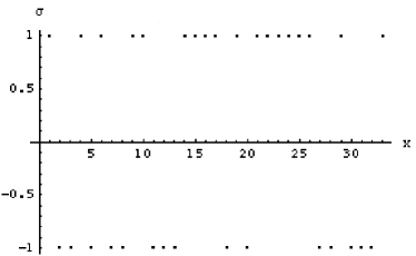
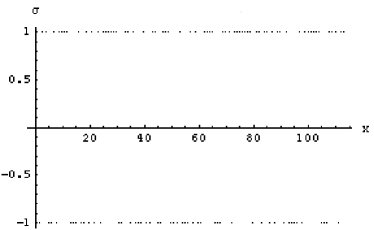
Figure 1: Ground state for $N=33$ and $N=113$

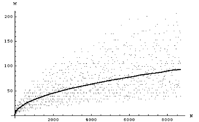
Figure 2: Total magnetization $Nm^{0}$ of the ground state versus $N$, $2N+1=4m+3$ prime. The continuous curve is $\sqrt{N}$.

For the remaining part of the paper we will restrict to $p=2N+1$ prime, with $p=3\,(\mbox{mod}4)$. We point out that this set has measure zero as a subset of the natural numbers. However, we have strong numerical evidence that some relevant properties that we are going to discuss hereafter, such as the behaviour of $m^{0}(N)$, the statistics of energy levels and the number of metastable states (see below) are somehow generic in $N$.

Let $\Omega_{s}\subset\Sigma_{N}$ be the subspace consisting of the ${N\choose s}$ configurations obtained by starting from the ground state $\sigma^{0}$ described above and flipping exactly $s$ different spins. Each point of $\Omega_{s}$ can thus be identified with a $s$-dimensional vector $\tau\in\{1,\dots,N\}^{s}$ of the form $\tau=(x_{1},\dots,x_{s})$, with $x_{i}\neq x_{j}$ for $i\neq j$, which specifies the positions of the flipped spins along the chain of length $N$. We then define the ‘flipping’ map $L_{\tau}:\Sigma_{N}\to\Sigma_{N}$ as:

$$\left(L_{\tau}\sigma\right)_{x}=\left\{\begin{array}[]{ll}-\sigma_{x},&x\in{\tau},\\ \;\;\,\sigma_{x},&x\notin{\tau}.\end{array}\right.$$ (4.17)

In this way we can write

$$\Omega_{s}=\{L_{\tau}\sigma^{0}\}_{\tau}.$$ (4.18)

The correspondence $\tau\to\sigma$ given by $\sigma=L_{\tau}\sigma^{0}$ is plainly one-to-one. Therefore in the sequel we shall freely identify a state $\sigma=L_{\tau}\sigma^{0}$ with the vector $\tau$. Alternatively, we can proceed as follows. Define the overlap $q(\sigma)$ of a given configuration $\sigma\in\Sigma_{N}$ with respect to the ground state $\sigma^{0}$ as:

$$q(\sigma)={1\over N}\sum_{x=1}^{N}\sigma_{x}\sigma_{x}^{0},$$ (4.19)

so that $q(\sigma^{0})=1$. Then

$$\Omega_{s}=\{\sigma\in\Sigma_{N}\,:\,q(\sigma)=1-2{s\over N}\}$$ (4.20)

The following straightforward calculation yields the energy values on the space $\Omega_{s}$: using the definition of $L_{\tau}$, the symmetry of $J$ and the fact that the ground state $\sigma^{0}$ is an eigenvector of $J$ to the eigenvalue $1$ we have:

$$H(L_{\tau}\sigma^{0}) = -\frac{1}{2}\sum_{x\in\tau}\sum_{y\in\tau}J_{xy}\sigma^{0}_{x}\sigma^{0}_{y}+\frac{1}{2}\sum_{x\in\tau}\sum_{y\notin\tau}J_{xy}\sigma^{0}_{x}\sigma^{0}_{y}$$ (4.21)

$$+\frac{1}{2}\sum_{x\notin\tau}\sum_{y\in\tau}J_{xy}\sigma^{0}_{x}\sigma^{0}_{y}-\frac{1}{2}\sum_{x\notin\tau}\sum_{y\notin\tau}J_{xy}\sigma^{0}_{x}\sigma^{0}_{y}$$

$$= -\frac{1}{2}\sum_{x,y=1}^{N}J_{xy}\sigma^{0}_{x}\sigma^{0}_{y}+2\sum_{x\in\tau}\sum_{y\notin\tau}J_{xy}\sigma^{0}_{x}\sigma^{0}_{y}$$

$$= -\frac{N}{2}+2\sum_{x\in\tau}\sum_{y=1}^{N}J_{xy}\sigma^{0}_{x}\sigma^{0}_{y}-2\sum_{x\in\tau}\sum_{y\in\tau}J_{xy}\sigma^{0}_{x}\sigma^{0}_{y}$$

$$= -\frac{N}{2}+2\sum_{x\in\tau}(\sigma^{0}_{x})^{2}-2\sum_{x\in\tau}\sum_{y\in\tau}J_{xy}\sigma^{0}_{x}\sigma^{0}_{y}$$

$$= -\frac{N}{2}+2s-2\sum_{x\in\tau}\sum_{y\in\tau}J_{xy}\sigma^{0}_{x}\sigma^{0}_{y}.$$

Notice that for the Ising mean-field interaction: $J_{xy}=1/N$, one finds

$$H(L_{\tau}\sigma^{0})=-\frac{N}{2}+2s-2\frac{s^{2}}{N}=-{N\over 2}\left(1-{2s\over N}\right)^{2}.$$ (4.22)

It is now possible to study the distribution of the energy levels on the individual subspaces $\Omega_{s}$, where $s=0,1,\ldots,N$. Let $p_{s}$ be the probability distribution restricted on $\Omega_{s}$, i.e.

$$p_{s}(C)={{N\choose s}}^{-1}\sum_{\sigma\in C\cap\Omega_{s}}1,$$ (4.23)

and let ${\rm E}\,_{s}$ denote the expectation wrt $p_{s}$. The $n$-th moment of the energy $H$ on the subspace $\Omega_{s}$ is given by

$${\rm E}\,_{s}(H^{n})\equiv\int_{\Omega_{s}}H^{n}(\sigma)\,dp_{s}(\sigma)={{N\choose s}}^{-1}\sum_{\tau\in\Omega_{s}}H^{n}(L_{\tau}\sigma^{0}),$$ (4.24)

so that the $n$-th moment ${\rm E}\,_{N}(H^{n})$ of the energy on the whole configuration space $\Sigma_{N}$ is

$${\rm E}\,_{N}(H^{n})\equiv\int_{\Sigma_{N}}H^{n}(\sigma)\,d{\rm P}\,_{N}(\sigma)={1\over 2^{N}}\sum_{s=0}^{N}{N\choose s}\,{\rm E}\,_{s}(H^{n}).$$ (4.25)

A tedious but straightforward calculation (see Appendix) yields the following expressions for the first two $s$-moments:

$${\rm E}\,_{s}(H)=\,-{N\over 2}\left(1-{2s\over N}\right)^{2},\qquad$$ (4.26)

$$\sigma_{s}^{2}(H)\equiv{\rm E}\,_{s}(H^{2})-({\rm E}\,_{s}(H))^{2}=\frac{4s(s-N)(2s^{2}-2sN+N)}{N^{2}(N-2)}$$ (4.27)

and consequently

$${\rm E}\,_{N}(H)=-{1\over 2},\qquad{\rm E}\,_{N}(H^{2})-({\rm E}\,_{N}(H))^{2}={N-1\over 2}.$$ (4.28)

These results indicate that, at variance with the ferromagnetic case where the energy is constant on each subspace $\Omega_{s}$, here there is a significant overlap between the distributions (for different $s$ values) of the energy when restricted to $\Omega_{s}$. In particular, from the espression of $\sigma_{s}^{2}$ we see that there can be a large number of states having small overlap with the ground state but nevertheless with energy very close to $-N/2$. For example we have $\sigma^{2}_{N/2}\simeq N/2$, indicating that the energy restricted to the subspace $\Omega_{N/2}$ may fluctuate over the whole energy range. This simple phenomenon is intimately related to the existence of metastable states and it will prove crucial in the understanding of the zero temperature dynamics, as discussed below. Fig. 3 shows the distributions of the energy restricted to various subspaces $\Omega_{s}$.

Figure 3: Distributions of the energy over the subspaces $\Omega_{s}$. The size of the system is $N=23$ and $s=3,4,\ldots,11$ from left to right

Another quantity of interest is the specific magnetization $m(\sigma)$ of an arbitrary state $\sigma\in\Sigma_{N}$, given by:

$$m(\sigma)={1\over N}\sum_{x=1}^{N}\sigma_{x},$$ (4.29)

In particular, given $\tau=(x_{1},\dots,x_{s})$, we have

$$m(L_{\tau}\sigma^{0})\,\equiv m(\tau)=\,m^{0}-\frac{2}{N}\sum_{x\in\tau}\left(\frac{x}{p}\right).$$ (4.30)

Clearly,

$$\frac{1}{\left(\begin{array}[]{c}N\\ s\end{array}\right)}\sum_{\tau\in\Omega_{s}}\left(\sum_{x\in\tau}\left(\frac{x}{p}\right)\right)\,=\,\frac{1}{\left(\begin{array}[]{c}N\\ s\end{array}\right)}\sum_{x=1}^{N}\left(\begin{array}[]{c}n-1\\ s-1\end{array}\right)\cdot\left(\frac{x}{p}\right)=\,s\cdot m^{0}\,,$$ (4.31)

i.e.

$$E_{s}(m)\,=\,\frac{1}{\left(\begin{array}[]{c}N\\ s\end{array}\right)}\sum_{\tau\in\Omega_{s}}m(\tau)\,=\,m^{0}\left(1-2{s\over N}\right).$$ (4.32)

Moreover, we show in the Appendix that

$$\sigma_{s}^{2}(m)\equiv E_{s}(m^{2})-(E_{s}(m))^{2}=\frac{4s(N-s)}{N^{3}(N-1)}+\frac{4s(s-1)}{N^{3}(N-1)}\cdot\sum_{x=1}^{p}\left(\frac{x}{p}\right)d_{N}(x),$$ (4.33)

where $d_{N}(x)$ is the integer valued function giving the number of elements $u\in\{1,\dots,N\}$ such that $u^{-1}x\in\{1,\dots,N\}$ (where $u^{-1}$ denotes the inverse $\hbox{\rm mod\ }p$ of $u$). As will be discussed in the Appendix, $d_{N}(x)$ takes values around $p/4$ with rather small fluctuations. Since $\sum_{x=1}^{p}\left(\frac{x}{p}\right)=0$, the last term in (4.33) can beconsidered as a small correction to the constant value $4s(N-s)/N^{3}(N-1)$.

5 Zero temperature dynamics and metastable states.

We first introduce the following discrete $1-$flip dynamics, given by:

$$\sigma(t+1)=\left\{\begin{array}[]{l}L_{\omega(t)}\,\,\sigma(t),\qquad\mbox{if $H(L_{\omega}\sigma)<H(\sigma)$,}\\ \ \qquad\sigma(t),\qquad\mbox{otherwhise,}\end{array}\right.$$

where, for each $t$, $\omega(t)$ is chosen randomly in $\{1,\ldots,N\}$ with uniform distribution. Choosing an initial condition $\sigma(0)$ at random with respect to ${\rm P}\,_{N}$, one obtains a random orbit $\{\sigma(0),\sigma(1),\ldots,\sigma(\ell)\}$ for any realization $\{\omega(t)\}_{1\leq t\leq\ell}$ of length $\ell$. As a consequence of the previous analysis, we have the following remarks.

• On one hand, it may happen that starting from $\sigma(0)$ one reaches after $t$ iterations a state $\sigma(t)\in\Omega_{s}$, of the form $\sigma(t)=L_{\tau}\sigma^{0}$ for some $\tau=(x_{1},\dots,x_{s})$, such that $H(L_{\tau}\sigma^{0})<H(L_{\omega}L_{\tau}\sigma^{0})$ for any $\omega\in\{x_{1},\dots,x_{s}\}$.

• On the other hand one can reach $\sigma(t)\in\Omega_{s}$ such that for some $\omega\in\{1,\dots,N\}$, $L_{\omega}\sigma\in\Omega_{s+1}$ and $H(L_{\omega}\sigma(t))<H(\sigma(t))$.

Due to the above observations, the overlap function $q(\sigma(t))$ is in general not monotonically non-decreasing along a given random orbit (this at variance with the Ising mean field model). In particular there might be metastable states [NS]. Now, given $\omega\in\{1,\dots,N\}$, we shall say that a configuration $\sigma\in\Sigma_{N}$ is $\omega$-stable if

$$H(L_{\omega}\sigma)\,>\,H(\sigma).$$ (5.34)

Moreover, we say that $\sigma$ is $1$-flip stable (or metastable) if it is $\omega$-stable $\forall\omega\in\{1,\ldots,N\}$.

We denote by $n(N)$ the total number of such metastable states as a function of $N$. From (4.21) one readily obtains that

$$H(L_{\omega}\sigma)\,=\,H(\sigma)\,+\,2\,\sum_{x\neq\omega}\,J_{x\omega}\,\sigma_{x}\,\sigma_{\omega},$$ (5.35)

so that $\sigma$ is $\omega$-stable if and only if

$$\left(J\sigma\right)_{\omega}\sigma_{\omega}>J_{\omega\omega}.$$ (5.36)

Summing over $\omega$ and using (2.4) we see that if $\sigma$ is $1$-flip stable then

$$<J\sigma,\sigma>\;>\;1.$$ (5.37)

Recalling the expression (2.2) of the Hamiltonian we see that a necessary condition for $\sigma\in\Sigma_{N}$ to be $1$-flip stable is that

$$H(\sigma)<{\rm E}\,_{N}(H)=-{1\over 2}\,\cdot$$ (5.38)

The main goal of this paper is to give an estimate of the number of metastable states for any given $N$. To this end we first performed some numerical investigations. For $N\leq 30$ we performed an exact enumeration of all configurations, whereas for larger $N$ we run the zero temperature dynamics described above (“deep quench”) for a number or realizations $\{\omega(t)\}$ as large as $10^{8}$ for bigger sizes, keeping track of the metastable states. As shown in Fig. 4, the growth of these states is exponential for generic values of the $N$.

Figure 4: The number of metastable states $n(N)$ for $N$. The line represents the best fit $n(N)\approx e^{\lambda N}$ with $\lambda\approx 0.28$ for values of $N$ such that $p=2N+1$ is a prime of the form $4m+3$ (filled points). Other points are for generic integer $N$.

The best numerical fit yields

$$n(N)\simeq C\cdot e^{0.28N}.$$ (5.39)

We remark that the same behaviour has been observed in [PP] for the Random Orthogonal Model; for spin glasses see [PP2]. We now proceed to give a partial justification of this result by means of probabilistic arguments.

Let $\tau=(x_{1},\dots,x_{s})$ and $\omega\in\{1,\dots,N\}$ be given. Using (5.35) and $J\sigma^{0}\,=\,\sigma^{0}$, it is easy to see that if $\omega\notin\tau$ (i.e. $L_{\omega}\sigma\in\Omega_{s+1}$)

$$H(L_{\omega}\sigma)\,=\,H(\sigma)\,+\,2\,\left(1-J_{\omega\omega}-2\,\sum_{x\in\tau}\,J_{x\omega}\,\sigma^{0}_{x}\,\sigma^{0}_{\omega}\right),$$

whereas, if $\omega\in\tau$ (i.e. $L_{\omega}\sigma\in\Omega_{s-1}$), we have

$$H(L_{\omega}\sigma)\,=\,H(\sigma)\,-\,2\,\left(1+J_{\omega\omega}-2\,\sum_{x\in\tau}\,J_{x\omega}\,\sigma^{0}_{x}\,\sigma^{0}_{\omega}\right).$$

If we define

$$h(\tau,\omega)\,=\sum_{x\in\tau}J_{x\omega}\,\sigma^{0}_{x}\sigma^{0}_{\omega},$$ (5.40)

we then see that a configuration $\sigma=L_{\tau}\sigma^{0}$ is $\omega$-stable if and only if

$$\left\{\begin{array}[]{lll}h(\tau,\omega)&<&{1\over 2}(1-J_{\omega\omega}),\qquad\mbox{\rm if }\omega\notin\tau,\\ \\ h(\tau,\omega)&>&{1\over 2}(1+J_{\omega\omega}),\qquad\mbox{\rm if }\omega\in\tau.\end{array}\right.$$ (5.41)

We now dwell upon the problem of characterising the behaviour of the function $h(\tau,\omega)$ so as the condition (5.41) can be effectively used to estimate the number of metasable states. Let us rewrite $h(\tau,\omega)$ in the form

$$h(\tau,\omega)=\frac{2}{\sqrt{p}}\sum_{x\in\tau}\,\xi_{x}(\omega),$$ (5.42)

where

$$\xi_{x}(\omega):=\left(\frac{\omega x}{p}\right)\,\,\sin\left(\frac{2\pi\omega x}{p}\right).$$ (5.43)

Now, having fixed $\tau$ and $x\in\tau$, we can view the function $\xi_{x}(\omega)$ defined in (5.43) as a random variable uniformly distributed on $\{1,\dots,N\}$ and taking values in $[-1,1]$. Its mean $\mu_{x}$ and variance $\sigma^{2}_{x}$ are easily computed:

$$\mu_{x}={1\over N}\sum_{\omega=1}^{N}\left(\frac{\omega x}{p}\right)\,\,\sin\left(\frac{2\pi\omega x}{p}\right)={\sqrt{p}\over 2N},$$ (5.44)

and, using (2.4),

$$\sigma^{2}_{x}={1\over N}\sum_{\omega=1}^{N}\,\sin^{2}\left(\frac{2\pi\omega x}{p}\right)-\mu^{2}_{x}={p\over 4N}\left(1-{1\over N}\right).$$ (5.45)

Here we want to study the behaviour of the sum $\eta(\tau,\omega):=\sum_{x\in\tau}\xi_{x}(\omega)$. We remark that this sum, and thus $h(\tau,\omega)=2\eta(\tau,\omega)/\sqrt{p}$, has to be regarded as a r.v. defined on the product of two probability spaces: for each fixed $\tau$, it is the sum of the i.i.d.r.v.’s $\xi_{x}(\omega)$ on the space $\{1,\dots,N\}$ with uniform distribution (this comes from the very definition of the zero temperature dynamics); on the other hand, for each fixed $\omega$, it can be regarded as a r.v. on $\Omega_{s}$ viewed as a probability space endowed with the distribution $p_{s}$. Its mean is given by (recall that the symbol ${\rm E}\,_{s}$ denotes the expectation wrt $p_{s}$):

$${\rm E}\,_{s}\eta = {{N\choose s}}^{-1}\sum_{\tau=(x_{1},\dots,x_{s})}\sum_{x\in\tau}\xi_{x}(\omega)={{N\choose s}}^{-1}\sum_{x=1}^{N}{N-1\choose s-1}\xi_{x}(\omega)$$

$$= {s\over N}\sum_{x=1}^{N}\xi_{x}(\omega)={s\sqrt{p}\over 2N}.$$

which does not depend on $\omega$ and equals $s$ times $\mu_{x}$. Along the same lines one shows that

$${\rm Var}_{s}\eta={sp\over 4N}\left(1-{s\over N}\right).$$ (5.47)

Notice that unlike the means, here we have ${\rm Var}_{s}\eta\neq s\cdot\sigma_{x}^{2}$. This discrepancy comes from the fact that, for any fixed $\omega$, the sequence $\xi_{x_{1}},\xi_{x_{2}},\dots,\xi_{x_{s}}$ is a sequence of distinct (and ordered) elements so that by no means we can view $\eta$ as a sum of independent and identically distributed objects. Nonetheless, also supported by strong numerical evidence (see Fig. 5), we claim that a version of the central limit theorem is applicable so that when $N\to\infty$, $s\to\infty$ with $s/N\to\lambda$, we have

$$p_{s}\left(\alpha<{\eta-{\rm E}\,_{s}\eta\over\,\sqrt{{\rm Var}_{s}\eta}}<\beta\right)\rightarrow{1\over\sqrt{2\pi}}\int_{\alpha}^{\beta}e^{-y^{2}/2}\,dy.$$ (5.48)

Assuming the validity of (5.48), performing the change of variables $y=(x-\lambda)/\sqrt{\gamma}$, with $\gamma=\lambda(1-\lambda)$, and setting $a=\lambda+\alpha\sqrt{\gamma}$, $b=\lambda+\beta\sqrt{\gamma}$, we thus obtain an asymptotic gaussian distribution for $h(\,\cdot\,,\omega)$:

$$p_{s}\left(a<h(\tau,\omega)<b\right)\rightarrow{1\over\sqrt{2\pi\gamma}}\int_{a}^{b}e^{-(x-\lambda)^{2}/2\gamma}\,dx.$$ (5.49)

Note that the r.h.s. does not depend on $\omega$. One can actually say more: for any ${\tilde{\omega}},\omega\in\{1,\ldots,N\}$ we have $h({\tilde{\omega}}^{-1}\tau,{\tilde{\omega}}\omega)=h(\tau,\omega)$. Therefore the set of values of $h(\,\cdot\,,\omega)$ on $\Omega_{s}$ does not depend on the choice of $\omega$, i.e. $\left\{h(\tau,\omega)\right\}_{\tau\in\Omega_{s}}\,=\,\left\{h(\tau^{\prime},\omega^{\prime})\right\}_{\tau^{\prime}\in\Omega_{s}}$, for all $\omega$, $\omega^{\prime}$.

Figure 5: Distribution of the function $h(\tau,\omega)$ for a fixed $\omega\in\{1,\dots,N\}$ and $\tau$ varying in $\Omega_{s}$. Here $N=23$ and $s=3$ (left) and $s=11$ (right). The solid line is the gaussian distribution in the r.h.s. of (5.49).

Having fixed an order for the lattice points $(\omega_{1},\ldots,\omega_{N})$, $\omega_{j}\neq\omega_{k}$, we now consider the following quantities:

$$\pi_{s,N}(\omega_{k})=p_{s}\left(\left\{\sigma\in\Omega_{s}\,:\,H(L_{\omega_{k}}\sigma)\,>\,H(\sigma)\right\}\right),$$ (5.50)

the $p_{s}$-probability that a randomly chosen state $\sigma\in\Omega_{s}$ is $\omega_{k}$-stable,

$$\pi_{s,N}(\omega_{k+1}|\,\omega_{1},\ldots,\omega_{k}) = p_{s}\left(\left\{\sigma\in\Omega_{s}\,:\,H(L_{\omega_{k+1}}\sigma)\,>\,H(\sigma)\right.\right.$$ (5.51)

$$\;\;\;\;\;\;\;\left.\left.|\,H(L_{\omega_{j}}\sigma)\,>\,H(\sigma),\;\omega_{j}=\omega_{1},\ldots\omega_{k}\right\}\right),$$

the conditional $p_{s}$-probability that a randomly chosen state $\sigma\in\Omega_{s}$ is $\omega_{k+1}$-stable given that it is $\omega_{j}$-stable for $j=1,\ldots,k$, and

$$\pi_{s,N}=p_{s}\left(\left\{\sigma\in\Omega_{s}\,:\,H(L_{\omega}\sigma)\,>\,H(\sigma),\;\omega=\omega_{1},\dots,\omega_{N}\right\}\right),$$ (5.52)

the $p_{s}$-probability that a randomly chosen state $\sigma\in\Omega_{s}$ is $1$-flip stable (i.e. stable for all possible flipping). Notice that by condition (5.41) the last quantity can be written as

$$\pi_{s,N}={N\choose s}^{-1}\sum_{(x_{1},\dots,x_{s})=\tau\atop(y_{1},\dots,y_{N-s})=\tau^{c}}\prod_{i=1}^{s}\theta\left(h(\tau,x_{i})>{1+J_{x_{i}x_{i}}\over 2}\right)\,\prod_{j=1}^{N-s}\theta\left(h(\tau,y_{j})<{1-J_{y_{i}y_{i}}\over 2}\right).$$ (5.53)

The three quantities introduced above are related by the following identity:

$$\pi_{s,N}\,=\,\pi_{s}(\omega_{1})\cdot\pi_{s}(\omega_{2}|\omega_{1})\cdot\pi_{s}(\omega_{3}|\omega_{1},\omega_{2})\cdots\pi_{s}(\omega_{N}|\omega_{1},\ldots,\omega_{N-1})$$ (5.54)

and the total number of $1$-flip stable states in $\Sigma_{N}$ is, by definition,

$$n(N)=\sum_{s=0}^{N}{N\choose s}\pi_{s,N}.$$ (5.55)

We shall study the quantity $n(N)$ in the thermodynamic limit: $N\to\infty$, $s\to\infty$, with $s/N\to\lambda$ and $0<\lambda<1$. In this regime we write $\pi_{s,N}\equiv\pi_{\lambda}$ and apply Stirling’s formula to obtain

$${N\choose s}\sim{e^{NF(\lambda)}\over\sqrt{2\pi N\lambda(1-\lambda)}}\,,\quad\hbox{with}\quad F(\lambda)=-\lambda\log{\lambda}-(1-\lambda)\log{(1-\lambda)}.$$ (5.56)

Note that $F(\lambda)$ is concave and symmetric around $\lambda=1/2$, with $F(1/2)=\log 2$. In this way we get for $N$ large and $s\simeq\lambda N$ with $\lambda$ ranging in the unit interval,

$$n(N)\simeq\int_{0}^{1}{\sqrt{N\over 2\pi\lambda(1-\lambda)}}\,\exp{\biggl{[}N\biggl{(}F(\lambda)+{\log\pi_{\lambda}\over N}\biggr{)}\biggr{]}}\,d\lambda.$$ (5.57)

It thus remains to estimate the probability $\pi_{\lambda}$. Let us consider first the unconditioned probability (5.50). According to (5.41) and the total probability formula we have:

$$\pi_{s,N}(\omega_{k}) = {s\over N}\,p_{s}\left(h(\tau,\omega_{k})>{1+J_{\omega_{k}\omega_{k}}\over 2}\;\bigg{|}\;\tau\ni\omega_{k}\right)$$ (5.58)

$$+ \left(1-{s\over N}\right)\,p_{s}\left(h(\tau,\omega_{k})<{1-J_{\omega_{k}\omega_{k}}\over 2}\;\bigg{|}\;\tau\not\ni\omega_{k}\right).$$

Here $s/N$ and $1-s/N$ are the probabilities that $\tau\ni\omega_{k}$ and $\tau\not\ni\omega_{k}$, respectively. We can easily compute the conditional expectations

$${\rm E}\,(h|\tau\ni\omega_{k})={N-1\choose s-1}^{-1}{2\over\sqrt{p}}\sum_{\tau\ni\omega_{k}}\sum_{x\in\tau}\xi_{x}(\omega_{k})={s-1\over N-1}-\left({s-N\over N-1}\right)J_{\omega_{k}\omega_{k}}\,,$$ (5.59)

and

$${\rm E}\,(h|\tau\not\ni\omega_{k})={N-1\choose s}^{-1}{2\over\sqrt{p}}\sum_{\tau\not\ni\omega_{k}}\sum_{x\in\tau}\xi_{x}(\omega_{k})={s\over N-1}\left(1-J_{\omega_{k}\omega_{k}}\right)\,.$$ (5.60)

In a similar way one can compute the variances $\gamma_{+}(\omega_{k})$ and $\gamma_{-}(\omega_{k})$ conditioned to the events $\{\tau\ni\omega_{k}\}$ and $\{\tau\not\ni\omega_{k}\}$. For $N$ large and $s\simeq\lambda N$, retaining only terms ${\cal O}(1)$, one gets

$${\rm E}\,(h|\tau\ni\omega_{k})\simeq{\rm E}\,(h|\tau\not\ni\omega_{k})\simeq\lambda,\qquad\gamma_{-}(\omega_{k})\simeq\gamma_{+}(\omega_{k})\simeq\gamma=\lambda(1-\lambda).$$ (5.61)

Moreover in the thermodynamic limit specified above we write $\pi_{s,N}(\omega_{k})\equiv\pi_{\lambda}(\omega_{k})$ and argue from (5.49) the following approximate expression for $\pi_{\lambda}(\omega_{k})$:

$$\pi_{\lambda}(\omega_{k}) \simeq {\lambda\over\sqrt{2\pi\gamma}}\int_{1/2}^{\infty}e^{-(x-\lambda)^{2}/2\gamma}\,dx+{(1-\lambda)\over\sqrt{2\pi\gamma}}\int_{-\infty}^{1/2}e^{-(x-\lambda)^{2}/2\gamma}\,dx$$ (5.62)

$$= {1\over 2}+\left({1\over 2}-\lambda\right){\rm erf}\left({{1\over 2}-\lambda\over\sqrt{2\gamma}}\right)$$

where we have denoted the error function by

$${\rm erf}(z)={2\over\sqrt{\pi}}\int_{0}^{z}e^{-x^{2}}\,dx.$$ (5.63)

It is not difficult to check that the r.h.s. of (5.62) is convex and symmetrix around $\lambda=1/2$, where it reaches its minimum value equal to $1/2$.

Let us now come to $\pi_{s,N}$. In principle this quantity is to be computed by specifying the whole set of constraints embodied in (5.53) or, which is the same, by computing the conditional probabilities appearing in eq.(5.54). However, this appears to be a difficult task. A first approach which drastically simplifies this task is to forget about the constraints implied by (5.53) and assume that (in the thermodynamic limit) the various $\omega$-stability conditions become mutually independent, that is $\pi_{\lambda}(\omega_{k+1}|\omega_{1},\ldots,\omega_{k})=\pi_{\lambda}(\omega_{k+1})$, for all $k=1,\dots,N-1$, so that

$$\pi_{\lambda}=\prod_{k=1}^{N}\pi_{\lambda}(\omega_{k}).$$ (5.64)

Recalling eq. (5.57) and (5.62), one is led to the following expression for $n(N)$:

$$n(N)\simeq\int_{0}^{1}\sqrt{N\over 2\pi\lambda(1-\lambda)}\,\exp{\biggl{(}NG_{1}(\lambda)\biggr{)}}\,d\lambda,$$ (5.65)

where

$$G_{1}(\lambda)=F(\lambda)+\log{{1\over 2}+\left({1\over 2}-\lambda\right){\rm erf}\left({{1\over 2}-\lambda\over\sqrt{2\gamma}}\right)}$$ (5.66)

We show the shape of the the function $G_{1}(\lambda)$ in Fig. 6.

Figure 6: The function $G_{1}(\lambda)$ of equation (5.66) for $\lambda\in[0,1]$.

Evaluating the integral (5.65) with the saddle-point method one gets

$$n(N)\simeq C\,e^{0.14N}.$$ (5.67)

Notice that the exponent is the half of what is observed numerically (cfr (5.39)). In the remaining part of the paper we shall argue that (5.67) is indeed an estimate from below of the actual number of metastable states. The above discussion has been able to reproduce the exponential growth of the number of metastable states with the size of the system. To understand the discrepacy between the estimated exponent and the one measured numerically one should note that the nature of the interaction makes the conditional probabilities play a major role in the asymptotics of the number of metastable states. To be more precise, our approximation which assumes mutually independent individual $\omega$-stability events, i.e. $\pi_{\lambda}(\omega_{k+1}|\omega_{1},\ldots,\omega_{k})\simeq\pi_{\lambda}(\omega_{k+1})$, is actually reasonable only for small value of $k$ (this can be checked, for example, calculating the correlation functions). As numerical results shows, for large values of $k$ the specific form of the interactions make these events strongly dependent. In Fig. 7 we show the function $P(k)$ providing the average of $\pi_{\lambda}(\omega_{k+1}|\omega_{1},\ldots,\omega_{k})$ over a large sample of different permutations $(\omega_{1},\ldots,\omega_{N})$ of the lattice points. The conditional probabilities $P(k)$ grow monotonically, almost linearly, from the initial (unconditioned) value up to a number close to $1$. In other words, requiring that a large number $k$ of spins produce an $\omega$-stable state increases substantially the probability of doing the same for the remaining spins.

Figure 7: $P(k)$ versus $k$, for $N=15(\mbox{circle}),21(\mbox{square}),23(\mbox{diamonds})$ and $s=[N/2]$. The conditional probabilities have been averaged over a sample of $10000$ choices of $(\omega_{1},\ldots,\omega_{N})$.

Another way of understanding the constructive effect of the correlations is the following. Consider again the function $h(\tau,\omega)$. Having fixed $\omega_{k+1}$, we have already noticed that for $s$ and $N$ large enough the values of $h(\tau,\omega_{k+1})$ with $\tau\in\Omega_{s}$ are approximately distributed according to a gaussian probability density with mean $\lambda=s/N$ and variance $\gamma=\lambda(1-\lambda)$, regardless of the particular value of $\omega_{k+1}$. Thus, in particular, the same distribution are expected to arise if one considers the values of $h(\tau,\omega_{k+1})$ constrained to the subsets of configurations such that $\omega_{k+1}\in\tau$, or $\omega_{k+1}\notin\tau$. On the other hand, if one picks $\omega_{1},\omega_{2},\ldots,\omega_{k}$ with $\omega_{j}\neq\omega_{k+1}$, $j=1,\ldots,k$, and computes numerically the two conditional distributions of the values of $h(\tau,\omega_{k+1})$ given $\omega_{1}$-stability, … , $\omega_{k}$-stablity (again with the constraints $\omega_{k+1}\in\tau$ or $\omega_{k+1}\notin\tau$), one finds that their means move to opposite directions, thus increasing the probability of $\omega_{k+1}$-stability (see (5.58)). This is shown in Fig. 8, where a system of size $N=21$ and $s=10$ is considered. The two central distributions correspond to the unconditioned cases, namely the values of $h(\tau,\omega)$ for $\tau\in\Omega_{10}$ with the only constraints $\omega\in\tau$ or $\omega\notin\tau$, respectively. Considering instead the values taken by $h$ on the states $\tau$ which, besides the constraints specified above, are stable with respect the first $10$ spins, one finds two distributions whose mean values have moved towards opposite directions. An averaged over $\omega$ has been performed.

Figure 8: Graphs of the four distributions of the values of $h$ described in the text.

6 Conclusion

We have investigated the statistical properties of energy levels and metastables states for a class of deterministic models, the most representative being the sine model[MPR], which have attracted much attention in recent years for their glassy behaviour despite the non-random nature of the interaction. We have pushed further on the analogy with glassy systems, proving a number of properties typical of disordered spin models. In particular, using number theoretic methods, we have described the energy (equivalently, free energy at $T=0$) landscape as a function of configurations with a fixed overlap with the ground state. The analysis revealed the existence of states very different from the ground state but with energy arbitrarily close to it: this corresponds to the “chaoticity” property of spin-glasses systems, well established in long range models. More importantly, some of these states can be local energy minima (equivalently, $1$-flip stable at $T=0$). They are expected to have a significant weight on the partition function in the low-temperature region, giving rise to the non-equibrium behaviour observed in annealing Montecarlo experiments. We have been able to estimate the approximate number of these energy minima. The analytic computations, combined with the numerical findings, strongly support the conclusion that the bound (5.67) estimates from below the number of metastable states $n(N)$, proving their exponential increase with the size of the system.

A number of basic questions about metastability arises now in a natural way, such as computing the energy density distributions of metastables states, studying energy barriers among them and their attraction basins. Stability of configurations with respect to the flip of an arbitrary number of spins is an interesting question as well. These problems are currently under investigation using the approach developed in this paper and will be addressed elsewhere.

Appendix

• (Proof of (4.15)) Choose $N$ odd such that $p=2N+1$ is prime of the form $4m+3$, where $m$ is an integer. Denote by $\sigma^{0}$ the spin configuration given by the sequence of Legendre symbols, i.e.

  $$\sigma^{0}_{x}=\left(\frac{x}{p}\right)=\left\{\begin{array}[]{ll}+1,&\mbox{if $x=k^{2}(\bmod p)$},\\ -1,&\mbox{if $x\neq k^{2}(\bmod p)$},\end{array}\right.$$

  with $k=1,2,\ldots,p-1$. Let us show that $\sigma^{0}=(\sigma_{1}^{0}\ldots\sigma_{N}^{0})$ is the ground state for the sine model or, which is the same, that $\sigma^{0}$ is an eigenvector of $J$ with eigenvalue $1$. For basic results of number theory used in the proof see, for example, ref. [Ap].

  $$(J\sigma^{0})_{y} = \frac{2}{\sqrt{p}}\sum_{x=1}^{N}\sin\left(\frac{2\pi xy}{p}\right)\left(\frac{x}{p}\right)$$

  $$= \frac{2}{\sqrt{p}}\sum_{x=1}^{N}\frac{1}{2i}\left(\exp\left(\frac{i2\pi xy}{p}\right)\left(\frac{x}{p}\right)-\exp\left(\frac{-i2\pi xy}{p}\right)\left(\frac{x}{p}\right)\right)$$

  changing $$x\mapsto-x$$ in the second summation

  $$= \frac{1}{i\sqrt{p}}\left[\sum_{x=1}^{N}\exp\left(\frac{i2\pi xy}{p}\right)\left(\frac{x}{p}\right)-\sum_{x=-N}^{-1}\exp\left(\frac{i2\pi xy}{p}\right)\left(\frac{-x}{p}\right)\right]$$

  $$\mbox{using multiplicativity of Legendre symbols:}\left(\frac{-x}{p}\right)=\left(\frac{-1}{p}\right)\left(\frac{x}{p}\right)$$

  and the fact that $$\left(\frac{-1}{p}\right)=-1 p=3(\bmod 4)$$ if

  $$= \frac{1}{i\sqrt{p}}\left[\sum_{x=1}^{N}\exp\left(\frac{i2\pi xy}{p}\right)\left(\frac{x}{p}\right)+\sum_{x=-N}^{-1}\exp\left(\frac{i2\pi xy}{p}\right)\left(\frac{x}{p}\right)\right]$$

  $$\mbox{using the periodicity of Legendre' symbols}:\,\left(\frac{x+p}{p}\right)=\left(\frac{x}{p}\right)$$

  $$= \frac{1}{i\sqrt{p}}\left[\sum_{x=1}^{N}\exp\left(\frac{i2\pi xy}{p}\right)\left(\frac{x}{p}\right)+\sum_{x=N+1}^{2N}\exp\left(\frac{i2\pi xy}{p}\right)\left(\frac{x}{p}\right)\right]$$

  being $$\left(\frac{p}{p}\right)=0$$ by definition

  $$= \frac{1}{i\sqrt{p}}\sum_{x=1}^{p}\exp\left(\frac{i2\pi xy}{p}\right)\left(\frac{x}{p}\right)$$

  using the separability for Gauss sums

  $$= \frac{1}{i\sqrt{p}}\left(\frac{y}{p}\right)\sum_{x=1}^{p}\exp\left(\frac{i2\pi x}{p}\right)\left(\frac{x}{p}\right)$$

  evaluating the Gauss sum

  $$= \frac{1}{i\sqrt{p}}\left(\frac{y}{p}\right)i\sqrt{p}\;=\;\sigma^{0}_{y}\,,\qquad\qquad\qquad\qquad$$

  which is the desired property.

• (Proof of (4.26) and (4.27)) We sketch the basic steps of the calculation. Set

  $$\alpha=-\frac{N}{2}+2s~{}~{}~{}~{}~{}~{}~{}~{}~{}~{}~{}~{}~{}~{}c_{j}=\left(\begin{array}[]{c}N-j\\ s-j\end{array}\right).$$

  We then have

  $${\rm E}\,_{s}(H^{n})={1\over c_{0}}\sum_{\tau\in\Omega_{s}}\left(\alpha-2\sum_{x\in\tau}\sum_{y\in\tau}J_{xy}\right)^{n}={1\over c_{0}}\sum_{\tau\in\Omega_{s}}\sum_{k=0}^{n}\left(\begin{array}[]{c}n\\ k\end{array}\right)\alpha^{n-k}\left(-2\sum_{x\in\tau}\sum_{y\in\tau}J_{xy}\right)^{k}.$$

  For $n=1$ we get

  $$\sum_{\tau\in\Omega_{s}}\left(\sum_{x\in\omega}\sum_{y\in\omega}J_{xy}\right) = \sum_{x=1}^{N}\sum_{y\neq x,y=1}^{N}c_{2}J_{xy}\sigma_{x}\sigma_{y}+\sum_{x=1}^{N}c_{1}J_{xx}$$

  $$= \sum_{x=1}^{N}\sum_{y=1}^{N}c_{2}J_{xy}\sigma_{x}\sigma_{y}+\sum_{x=1}^{N}(c_{1}-c_{2})J_{xx}=c_{2}(N-1)+c_{1},$$

  whereas for $n=2$ we have

  $$\sum_{\omega\in\Omega_{s}}\left(\sum_{x\in\omega}\sum_{y\in\omega}J_{xy}\right)^{2}=\sum_{z=1}^{N}\sum_{u\neq z;u=1}^{N}J_{zu}\sigma_{z}\sigma_{u}\left[\sum_{x\neq z,u;x=1}^{N}\sum_{y\neq z,u,x;y=1}^{N}c_{4}J_{xy}\sigma_{x}\sigma_{y}\right.$$

  $$+ \sum_{y\neq z,u;y=1}^{N}c_{3}J_{zy}\sigma_{z}\sigma_{y}+\sum_{y\neq z,u;y=1}^{N}c_{3}J_{uy}\sigma_{u}\sigma_{y}+\sum_{x\neq z,u;x=1}^{N}c_{3}J_{xz}\sigma_{x}\sigma_{z}+\sum_{x\neq z,u;x=1}^{N}c_{3}J_{xu}\sigma_{x}\sigma_{u}$$

  $$+ \left.\sum_{x\neq z,u;x=1}^{N}c_{3}J_{xx}+c_{2}J_{zu}\sigma_{z}\sigma_{u}+c_{2}J_{zz}+c_{2}J_{uu}\right]+\sum_{z=1}^{N}J_{zz}\left[\sum_{x\neq z;x=1}^{N}\sum_{y\neq z,x;y=1}^{N}c_{3}J_{xy}\sigma_{x}\sigma_{y}\right.$$

  $$+ \sum_{x\neq z;x=1}^{N}c_{2}J_{xz}\sigma_{x}\sigma_{z}\left.+\sum_{y\neq z;y=1}^{N}c_{2}J_{yz}\sigma_{y}\sigma_{z}+\sum_{x\neq z;x=1}^{N}c_{2}J_{xx}+c_{1}J_{zz}\right]$$

  $$= c_{4}(N-1)(N-3)+2c_{3}(N-1)+2c_{2}(N-1)+c_{1},$$

  which easily give the desired identities.

• (Proof of (4.33)) Let us first extend everything to the set $\{1,2,\ldots,p-1\}$ which, $p$ being prime, is a number field. Here we can exploit the multiplicative structure of the field and of the ‘extended ground state’ $\sigma^{0}_{x}=\left(\frac{x}{p}\right)$, $x=1,\ldots,q$, with $q=p-1$. With slight abuse of notation we shall use the same symbols $\Omega_{s}$, $p_{s}$ and ${\rm E}\,_{s}$ to denote the corresponding extended quantities. It is immediate to see that $m(\sigma^{0})=0$ and

  $$E_{s}(m)\,=\,\frac{1}{\left(\begin{array}[]{c}q\\ s\end{array}\right)}\sum_{\tau\in\Omega_{s}}\left(\frac{-2}{q}\sum_{x\in\tau}\left(\frac{x}{p}\right)\right)=0.$$

  In order to calculate the second moment we consider

  $$\frac{1}{\left(\begin{array}[]{c}q\\ s\end{array}\right)}\sum_{\tau\in\Omega_{s}}\left(\sum_{x\in\tau}\left(\frac{x}{p}\right)\right)^{2}\, = \,\frac{1}{\left(\begin{array}[]{c}q\\ s\end{array}\right)}\sum_{\tau\in\Omega_{s}}\left(\sum_{x\in\tau^{2}}\left(\frac{x}{p}\right)\right)$$

  $$= \frac{1}{\left(\begin{array}[]{c}q\\ s\end{array}\right)}\sum_{x=1}^{q}c_{p}(x)\,\left(\frac{x}{p}\right)\,,$$

  where, for any given $\tau\in\Omega_{s}$, $\tau^{2}$ is the collection, with multiplicity, of all possible products $x_{j}\cdot x_{i}$, $x_{i},x_{j}\in\tau$ (all the operations are $\mbox{mod }p$). For example, if $\tau=\{x_{1},x_{2},x_{3}\}$ then $\tau^{2}=\{x_{1}^{2},x_{2}^{2},x_{3}^{2},x_{1}x_{2},x_{1}x_{3},x_{2}x_{1},x_{3}x_{1},x_{2}x_{3},x_{3}x_{2}\}$. Also, for any given $x\in\{1,\ldots,q\}$,

  $$c_{p}(x)\,=\,\sum_{\tau\in\Omega_{s}}\{\mbox{number of times }x\in\tau^{2}\}=\sum_{u=1}^{q}\sharp\{\tau\,|\,u\in\tau\mbox{ and }u^{-1}x\in\tau\}.$$

  In particular, if $\left(\frac{x}{p}\right)=-1$ then $u\neq u^{-1}x$, $\forall u=1,\ldots,q$, therefore

  $$c_{p}(x)\,=\,\sum_{u=1}^{q}\left(\begin{array}[]{c}q-2\\ s-2\end{array}\right)\,=\,q\left(\begin{array}[]{c}q-2\\ s-2\end{array}\right).$$

  If instead $\left(\frac{x}{p}\right)=1$, then there exists ${\bar{u}}$ such that ${\bar{u}}^{2}=x$, i.e.

  $$c_{p}(x)\,=\,\sum_{u\neq\pm{\bar{u}}}\left(\begin{array}[]{c}q-2\\ s-2\end{array}\right)+2\left(\begin{array}[]{c}q-1\\ s-1\end{array}\right)\,=\,(q-2)\left(\begin{array}[]{c}q-2\\ s-2\end{array}\right)+2\left(\begin{array}[]{c}q-1\\ s-1\end{array}\right).$$

  Putting everything together we get the following expression for the variance $\sigma^{2}_{s}(m)$:

  $$\sigma^{2}_{s}(m) = \frac{4}{q^{2}\left(\begin{array}[]{c}q\\ s\end{array}\right)}\sum_{\tau\in\Omega_{s}}\left(\sum_{x\in\tau}\left(\frac{x}{p}\right)\right)^{2}$$

  $$= \frac{4}{q^{2}\left(\begin{array}[]{c}q\\ s\end{array}\right)}\left[-\frac{q^{2}}{2}\left(\begin{array}[]{c}q-2\\ s-2\end{array}\right)+\frac{q}{2}(q-2)\left(\begin{array}[]{c}q-2\\ s-2\end{array}\right)+q\left(\begin{array}[]{c}q-1\\ s-1\end{array}\right)\right]$$

  $$= \frac{4}{q\left(\begin{array}[]{c}q\\ s\end{array}\right)}\left[\left(\begin{array}[]{c}q-1\\ s-1\end{array}\right)-\left(\begin{array}[]{c}q-2\\ s-2\end{array}\right)\right]={4s(q-s)\over q^{2}(q-1)}.$$

  We now turn back to our the original lattice $\{1,\dots,N\}$. Again we can write

  $$\frac{1}{\left(\begin{array}[]{c}N\\ s\end{array}\right)}\sum_{\tau\in\Omega_{s}}\left(\sum_{x\in\tau}\left(\frac{x}{p}\right)\right)^{2}\,=\,\frac{1}{\left(\begin{array}[]{c}N\\ s\end{array}\right)}\sum_{x=1}^{p}c_{N}(x)\left(\frac{x}{p}\right).$$

  In this case, however, the multiplicity function $c_{N}(x)$ can not be handled as easily as before. In particular, given $x\in\{1,\ldots N\}$, we denote by $\Gamma(x)$ the set $=\{u_{1},\ldots,u_{d_{N}(x)}\}$ given by the $u$’s in $\{1,\ldots,N\}$ such that $u^{-1}x\in\{1,\ldots,N\}$. The cardinality $d_{N}(x)$ of the set $\Gamma(x)$ is a non trivial function of $x$. It is shown in Fig. 9 for $1\leq x\leq N$. If now $\left(\frac{x}{p}\right)=-1$, then clearly

  $$c_{N}(x)\,=\,d_{N}(x)\cdot\left(\begin{array}[]{c}N-2\\ s-2\end{array}\right).$$

  On the other hand, if $\left(\frac{x}{p}\right)=1$ (i.e. ${\bar{u}}^{2}=x$), then (note that either ${\bar{u}}\in\{1,\ldots,N\}$ or $-{\bar{u}}\in\{1,\ldots,N\}$)

  $$c_{N}(x)\,=\,(d_{N}(x)-1)\cdot\left(\begin{array}[]{c}N-2\\ s-2\end{array}\right)+\left(\begin{array}[]{c}N-1\\ s-1\end{array}\right).$$

  

  

  Figure 9: The function $d_{N}(x)$ versus $x$, for $N=551$ and $N=933$

  We can then use these informations and write

  $$\frac{1}{\left(\begin{array}[]{c}N\\ s\end{array}\right)}\sum_{\tau\in\Omega_{s}}\left(\sum_{x\in\tau}\left(\frac{x}{p}\right)\right)^{2} = \frac{1}{\left(\begin{array}[]{c}N\\ s\end{array}\right)}\sum_{x=1}^{p}c_{N}(x)\,\left(\frac{x}{N}\right)$$

  $$= \frac{1}{\left(\begin{array}[]{c}N\\ s\end{array}\right)}\left[-\sum_{\left(\frac{x}{p}\right)=-1}d_{N}(x)\cdot\left(\begin{array}[]{c}N-2\\ s-2\end{array}\right)\,+\right.$$

  $$\left.+\,\sum_{\left(\frac{x}{p}\right)=1}\left(\,(d_{N}(x)-1)\cdot\left(\begin{array}[]{c}N-2\\ s-2\end{array}\right)+\left(\begin{array}[]{c}N-1\\ s-1\end{array}\right)\,\right)\right]$$

  $$= \frac{1}{\left(\begin{array}[]{c}N\\ s\end{array}\right)}\left[\left(\begin{array}[]{c}N-2\\ s-2\end{array}\right)\cdot\sum_{x=1}^{p}d_{N}(x)\left(\frac{x}{p}\right)+\right.$$

  $$\left.+\left(\left(\begin{array}[]{c}N-1\\ s-1\end{array}\right)-\left(\begin{array}[]{c}N-2\\ s-2\end{array}\right)\right)\cdot\sum_{\left(\frac{x}{p}\right)=1}1\right].$$

  Finally, we have the following expression for the variance $\sigma_{s}^{2}(m)$ of the magnetization $m$ over the space $\Omega_{s}$:

  $$\sigma_{s}^{2}(m)=\frac{4}{N^{2}}\,{\rm E}\,_{s}\left(\biggl{(}\sum_{x\in\tau}\left(\frac{x}{p}\right)\biggr{)}^{2}\right)\,-\,{4s^{2}(m^{0})^{2}\over N^{2}},$$

  from which one easily gets formula (4.33).

References

- [KTW] T.R.Kirkpatrick, P.G.Wolynes, Phys. Rev. A 35 (1987), 3072 Phys. Rev. B 36 (1987), 8552 T.R.Kirkpatrick, D.Thirumalai, Phys. Rev. B 36 (1987), 5388 Phys. Rev. B 38 (1988), 4881 For a review see also T.R.Kirkpatrick, D.Thirumalaii, Transp. Theor. Stat. Phys. 24 (1995), 927
- [SW] F. H. Stillinger, T. A. Weber, Science 225 (1984), 983
- [MP] M.Mèzard and G. Parisi, Statistical physics of structural glasses cond-mat/0002128
- [MPR] E.Marinari, G.Parisi and F.Ritort, J. Phys. A: Math. Gen. 27 (1994), 7615. E.Marinari, G.Parisi and F.Ritort, J.Phys. A: Math. Gen. 27 (1994), 7647
- [BM] J.P.Bouchaud and M.Mézard, J. Physique I 4 (1994), 1109
- [BDGU] I.Borsari, M.Degli Esposti, S.Graffi and F.Unguendoli, J. Phys. A: Math. Gen. 30 (1997), L155
- [NM] M.E.J. Newman and C.Moore, Glassy dynamics and aging in an exactly solvable spin model, Preprint 1997, cond-mat/9707273
- [PP] G Parisi, M Potters, J.Phys. A: Math. Gen. 28 (1995), 5267-5285.
- [PP2] G Parisi, M Potters, Europhysics Letters 32 (1995), 13-17.
- [MPV] M.Mézard, G.Parisi and M. Virasoro, Spin Glass Theory and Beyond, World Scientific 1995 (Singapore)
- [TE] F.Tanaka and S.F.Edwards, J.Phys. F 10 (1980), 2769
- [BrM] A.J.Bray and M.A.Moore, J.Phys C: Solid State Phys. 13 (1980), L469
- [DGGO] C. De Dominicis, M. Gabay, T. Garel and H. Orland J. Phys. (Paris) 41 (1980), 923
- [OF] V.M. de Oliveira and J.F.Fontanari,s J.Phys. A: Math. Gen. 30 (1997),8445
- [NS] C M Newman, D L Stein, Metastable states in spin glasses and disordered ferromagnets, Preprint 1999, cond-mat/9908455.
- [Ap] T. Apostol, Introduction to Analytic Number Theory, New York, Springer 1976
- [Si] Ya G Sinai, Probability Theory, Springer-Verlag 1991.