Conserving and gap-less model of the weakly interacting Bose gas

Abstract

The dielectric formalism is used to set up an approximate description of a spatially homogeneous weakly interacting Bose gas in the collision-less regime, which is both conserving and gap-less, and has coinciding poles of the single-particle Green’s function and the density autocorrelation function in the Bose-condensed regime. The approximation takes into account the direct and the exchange interaction in a consistent way. The fulfillment of the generalized Ward identities related to the conservation of particle-number and the breaking of the gauge-symmetry is demonstrated. The dynamics at long wavelengths is considered in detail below and above the phase-transition, numerically and in certain limits also in analytical approximations. The explicit form of the density autocorrelation function and the Green’s function is exhibited and discussed.

I Introduction

The observation of Bose-Einstein condensation [1] in trapped systems has given rise to an extensive experimental [2, 3] and theoretical [4] study of weakly interacting dilute Bose-condensed gases. Recent measurements of the elementary excitations [5, 6] permit the detailed comparison with different theoretical approaches. Due to the existence of a number of essential experimental parameters in the trapped systems, e.g. the trap frequencies, scattering length, size of the condensate and temperature, the validity of different approximations depending on these conditions can be examined. Most of the theoretical approaches go back to the 1960s, and were originally derived for spatially homogeneous systems in view of their application to superfluid helium. For their application to the modern Bose-Einstein condensates in traps many of these approaches are now being extended to inhomogeneous systems and new approaches are also being developed. In the present paper we wish to explore such a new approximation scheme. It is of interest for the modern Bose-Einstein condensates, because measurements of quasi-homogeneous properties can also be made there [7].

From the theoretical point of view taking the homogeneous limit implies a great simplification. Due to the translation symmetry complicated integral equations reduce to algebraic equations; essential requirements like a gap-less single-particle spectrum (which applies only in the homogeneous system) and the particle number conservation can be expressed in the form of algebraic identities (Hugenholtz Pines theorem [8], generalized Ward identities [9], compressibility sum-rule [10], etc.). In this form they provide important tests for the consistency of approximations obtained by selecting certain subsets of Feynman diagrams. Having defined an approximation or ‘model’ in this way analytical or numerical solution is possible in the spatially homogeneous case without the need for further approximation and all branches of the collective modes - damped, strongly damped and even over-damped (purely damped) - can be exhibited. This is a great advantage over the corresponding calculations for the spatially inhomogeneous system, where further approximations are unavoidable and a similarly complete picture usually cannot be attained.

The purpose of this paper is to examine the homogeneous limit of an approximation previously derived for and applied to the inhomogeneous case [11]. In contrast to the previous perturbative solution in the case of a harmonic trap [11] we shall now avoid all further approximations, after setting up the model by selecting the relevant class of Feynman diagrams, and derive and study all the excitation branches appearing in the homogeneous model. Furthermore, a number of exact theorems for the homogeneous system will be checked for their validity within our model approach.

For example, in general the poles of the density autocorrelation function and the single-particle Green’s function must coincide in the Bose-condensed region (see e.g. [12]). Physically this is a consequence of the existence of the order-parameter describing the spontaneously broken gauge-symmetry. In our approximation the required coincidence of the poles is a direct consequence of the derivation of the model within the dielectric formalism, which is designed to ensure just that. In contrast to a previous model studied within this formalism ([13], [12] and references therein) and therefore sharing this crucial property, the approximation or model studied here (and in [11] for the trapped system) takes into account the contributions of both the Hartree terms and the Fock (exchange) terms in the selected graphs. Both types of terms are in fact of equal magnitude for the interaction via $s$-wave scattering in the experimentally realized dilute weakly interacting Bose condensates.

In the next section we present the basic diagrammatic building blocks within the dielectric formalism as an approximation of the full system. The basic relations of the dielectric formalism are then used to obtain the final density autocorrelation and Green’s functions determining the excitation spectrum. We also state there the Generalized Ward identities, which are exact relations ensuring the particle number conservation law in cases of spontaneously broken symmetries. We prove in the appendix that these identities continue to hold in our model, which is a corner-stone of our model-building, because it provides an important consistency check. A further consistency check is the fulfillment of the compressibility sum-rule, which is demonstrated at the end of section II. In Section III we present the numerical results for the excitation branches at long wavelengths. Besides the modes we studied previously for the inhomogeneous system we find additional excitation branches belonging to excitations of mainly the thermal density. The behavior of these thermal branches will be studied in detail. For weak interaction they can be accurately approximated by simple analytic expressions, which is done in Section IV. For stronger interaction only numerical results are obtainable. They may suggest explanations for the appearance of the two different branches measured at JILA [14]. Section V contains some conclusions and further remarks.

II THE MODEL

A The dielectric formalism

Here we shall give some necessary background on the so-called ‘dielectric formalism’ at finite temperature, which was introduced for analyzing interacting Bose-condensed systems [15, 16, 13, 17, 18, 19, 12]. An excellent exposition of the formalism and a complete list of references is given by Griffin [12]. The presence of a Bose condensate breaks the gauge-symmetry of the system. As a consequence the density fluctuation spectra appear in the one particle excitation spectra and vice versa. In the dielectric formalism the corresponding coupling mechanism is explicitly exhibited.

For sake of simplification we adopt the natural unit $\hbar=1$ throughout the paper. In the Bose-condensed phase the usual decomposition of the Bose field operator $\hat{\Psi}$ in a condensate wave function $\Phi_{0}=\langle\hat{\Psi}(\mathchoice{{\hbox{\boldmath$\displaystyle r$}}}{{\hbox{\boldmath$\textstyle r$}}}{{\hbox{\boldmath$\scriptstyle r$}}}{{\hbox{\boldmath$\scriptscriptstyle r$}}})\rangle$ and the fluctuation operator $\hat{\Phi}$ with vanishing expectation value

$$\hat{\Psi}=\Phi_{0}+\hat{\Phi}$$ (1)

is made. $\langle\ldots\rangle$ denotes the thermal averaging

$$\langle\hat{A}\rangle={\mbox{Tr}\,\hat{A}e^{-\beta(\hat{H}-\mu\hat{N})}\over\mbox{Tr}\,e^{-\beta(\hat{H}-\mu\hat{N})}}.$$ (2)

The condensate wave function can in general be complex, but in the absence of vortices it can be chosen as real, without restriction of generality, and we shall consider this case in the following, for simplicity. The value of the chemical potential $\mu$ is fixed by the average number of particles in the system and is connected with the density of particles in the condensate $|\Phi_{0}|^{2}$ by requiring $\langle\hat{\Phi}\rangle=0.$ Imposing $\Phi_{0}\neq 0$ we have the additional appearance of anomalous Green’s functions and it is useful to introduce the matrix Green’s function

$$G_{\alpha\beta}(\mathchoice{{\hbox{\boldmath$\displaystyle r$}}}{{\hbox{\boldmath$\textstyle r$}}}{{\hbox{\boldmath$\scriptstyle r$}}}{{\hbox{\boldmath$\scriptscriptstyle r$}}},\tau;\mathchoice{{\hbox{\boldmath$\displaystyle r$}}}{{\hbox{\boldmath$\textstyle r$}}}{{\hbox{\boldmath$\scriptstyle r$}}}{{\hbox{\boldmath$\scriptscriptstyle r$}}}^{\prime},\tau^{\prime})=-\langle T_{\tau}\left[\hat{\Phi}_{\alpha}(\mathchoice{{\hbox{\boldmath$\displaystyle r$}}}{{\hbox{\boldmath$\textstyle r$}}}{{\hbox{\boldmath$\scriptstyle r$}}}{{\hbox{\boldmath$\scriptscriptstyle r$}}},\tau)\hat{\Phi}_{\beta}^{\dagger}(\mathchoice{{\hbox{\boldmath$\displaystyle r$}}}{{\hbox{\boldmath$\textstyle r$}}}{{\hbox{\boldmath$\scriptstyle r$}}}{{\hbox{\boldmath$\scriptscriptstyle r$}}}^{\prime},\tau^{\prime})\right]\rangle$$ (3)

with field operators in Matsubara representation $\hat{\Phi}_{1}(\mathchoice{{\hbox{\boldmath$\displaystyle r$}}}{{\hbox{\boldmath$\textstyle r$}}}{{\hbox{\boldmath$\scriptstyle r$}}}{{\hbox{\boldmath$\scriptscriptstyle r$}}},\tau)\equiv\hat{\Phi}(\mathchoice{{\hbox{\boldmath$\displaystyle r$}}}{{\hbox{\boldmath$\textstyle r$}}}{{\hbox{\boldmath$\scriptstyle r$}}}{{\hbox{\boldmath$\scriptscriptstyle r$}}},\tau)$ and $\hat{\Phi}_{2}(\mathchoice{{\hbox{\boldmath$\displaystyle r$}}}{{\hbox{\boldmath$\textstyle r$}}}{{\hbox{\boldmath$\scriptstyle r$}}}{{\hbox{\boldmath$\scriptscriptstyle r$}}},\tau)\equiv\hat{\Phi}^{\dagger}(\mathchoice{{\hbox{\boldmath$\displaystyle r$}}}{{\hbox{\boldmath$\textstyle r$}}}{{\hbox{\boldmath$\scriptstyle r$}}}{{\hbox{\boldmath$\scriptscriptstyle r$}}},\tau)$. In addition to these one particle correlation functions we need the density autocorrelation function:

$$\chi_{\rm nn}(\mathchoice{{\hbox{\boldmath$\displaystyle r$}}}{{\hbox{\boldmath$\textstyle r$}}}{{\hbox{\boldmath$\scriptstyle r$}}}{{\hbox{\boldmath$\scriptscriptstyle r$}}},\tau;\mathchoice{{\hbox{\boldmath$\displaystyle r$}}}{{\hbox{\boldmath$\textstyle r$}}}{{\hbox{\boldmath$\scriptstyle r$}}}{{\hbox{\boldmath$\scriptscriptstyle r$}}}^{\prime},\tau^{\prime})=-\langle T_{\tau}\left[\tilde{n}(\mathchoice{{\hbox{\boldmath$\displaystyle r$}}}{{\hbox{\boldmath$\textstyle r$}}}{{\hbox{\boldmath$\scriptstyle r$}}}{{\hbox{\boldmath$\scriptscriptstyle r$}}},\tau)\tilde{n}(\mathchoice{{\hbox{\boldmath$\displaystyle r$}}}{{\hbox{\boldmath$\textstyle r$}}}{{\hbox{\boldmath$\scriptstyle r$}}}{{\hbox{\boldmath$\scriptscriptstyle r$}}}^{\prime},\tau^{\prime})\right]\rangle.$$ (4)

Here $\tilde{n}=\hat{n}-\langle\hat{n}\rangle$ denotes the density deviation operator. The exact Green’s function $G_{\alpha\beta}$ can be obtained from Dyson’s equation, i.e. by summing up a geometric series in terms of the Green’s function $G^{0}_{\alpha\beta}$ of the noninteracting system and the self-energy $\Sigma_{\alpha\beta}$:

$$G_{\alpha\beta}=G^{0}_{\alpha\beta}+G^{0}_{\alpha\gamma}\Sigma_{\gamma\delta}G_{\delta\beta}.$$ (5)

The self-energy insertions are by definition irreducible i.e. cannot be split into two parts by cutting a single particle line. Different model approximations can be classified by the different kinds of interaction processes included in $\Sigma_{\alpha\beta}$.

Beyond the definition of irreducible quantities it is equally useful to consider the proper contributions. Diagrams are called proper if they cannot be split into two parts, each connected to an external vertex or line, by cutting a single interaction line. They will be denoted by an additional tilde. The total density autocorrelation function ${\chi_{\rm nn}}$ can be easily recovered from the proper contributions $\tilde{\chi}_{\rm nn}$ by just summing up a geometric series:

$$\chi_{\rm nn}(\mathchoice{{\hbox{\boldmath$\displaystyle q$}}}{{\hbox{\boldmath$\textstyle q$}}}{{\hbox{\boldmath$\scriptstyle q$}}}{{\hbox{\boldmath$\scriptscriptstyle q$}}},\omega)=\frac{\tilde{\chi}_{\rm nn}(\mathchoice{{\hbox{\boldmath$\displaystyle q$}}}{{\hbox{\boldmath$\textstyle q$}}}{{\hbox{\boldmath$\scriptstyle q$}}}{{\hbox{\boldmath$\scriptscriptstyle q$}}},\omega)}{1-g\tilde{\chi}_{\rm nn}(\mathchoice{{\hbox{\boldmath$\displaystyle q$}}}{{\hbox{\boldmath$\textstyle q$}}}{{\hbox{\boldmath$\scriptstyle q$}}}{{\hbox{\boldmath$\scriptscriptstyle q$}}},\omega)}.$$ (6)

Here $\omega$ on the one hand denotes the Matsubara-frequency [20] $\omega=i\omega_{\rm n}=i(2n\pi/\beta)$. On the other hand it is understood that the analytic continuation in $\omega$ from the positive imaginary axis yields the retarded correlation functions, and therefore, if this is our purpose, $\omega$ will in the following always be assumed to lie in the upper half of the complex plane. $g$ denotes the 2-particle T-matrix. In the whole temperature-domain of relevance here it can be taken as independent of $\bf{q},\omega$ and be expressed by the s-wave scattering length $a$ as

$$g=\frac{4\pi a}{m}$$ (7)

The importance of the use of the T-matrix in place of the bare interaction was first stressed in this context in Beliaev’s work [21]. (See [17] for a discussion of ladder diagrams within the dielectric formalism at finite temperature.) As is well known since then the use of the 2-particle T-matrix in place of the bare interaction implies that a sum is implicitly performed over the ladder-diagrams of the two-particle interaction, and care has to be taken not to sum up the same class of diagrams again later-on, see e.g. [22].

In the dielectric formalism the approximations for $\Sigma_{\alpha\beta}$ and for $\tilde{\chi}_{\rm nn}$ are related to each other via irreducible vertex functions $\Lambda_{\alpha}$ describing single processes of excitations out of the condensate and of relaxations into the condensate where the energy and momentum transfer is described by an additional out-going interaction line. Unlike in the usual Green’s function approach, where approximations are defined by the diagrams kept in the self-energies and $\tilde{\chi}_{\rm nn}$ as basic building blocks, in the dielectric formalism an approximation (or ‘model’) is defined by introducing building blocks for the proper and irreducible parts of the three quantities $\Sigma_{\alpha\beta}$, $\chi_{\rm nn}$ and $\Lambda_{\alpha}$. In the following we call irreducible and proper quantities to be regular and denote them with an $r$ in brackets.

Thus we start with specifying the building blocks ${\chi}_{\rm nn}^{(r)}$, ${\Sigma}_{\alpha\beta}^{(r)}$ and ${\Lambda}_{\alpha}^{(r)}$ and expressing all necessary quantities in terms of these three basic quantities, see e.g. [12]. We begin with the decomposition of the proper quantities $\tilde{G}_{\alpha\beta}$ and $\tilde{\chi}_{\rm nn}$. Since a Green’s function is proper if and only if all the self-energy insertions are proper we get

$$\tilde{G}_{\alpha\beta}^{-1}(\mathchoice{{\hbox{\boldmath$\displaystyle q$}}}{{\hbox{\boldmath$\textstyle q$}}}{{\hbox{\boldmath$\scriptstyle q$}}}{{\hbox{\boldmath$\scriptscriptstyle q$}}},\omega)=(G_{\alpha\beta}^{0})^{-1}(\mathchoice{{\hbox{\boldmath$\displaystyle q$}}}{{\hbox{\boldmath$\textstyle q$}}}{{\hbox{\boldmath$\scriptstyle q$}}}{{\hbox{\boldmath$\scriptscriptstyle q$}}},\omega)-{\Sigma}_{\alpha\beta}^{(r)}(\mathchoice{{\hbox{\boldmath$\displaystyle q$}}}{{\hbox{\boldmath$\textstyle q$}}}{{\hbox{\boldmath$\scriptstyle q$}}}{{\hbox{\boldmath$\scriptscriptstyle q$}}},\omega)$$ (8)

with $(G_{\alpha\beta}^{0})^{-1}(\mathchoice{{\hbox{\boldmath$\displaystyle q$}}}{{\hbox{\boldmath$\textstyle q$}}}{{\hbox{\boldmath$\scriptstyle q$}}}{{\hbox{\boldmath$\scriptscriptstyle q$}}},\omega)=\delta_{\alpha\beta}\left[\alpha\omega-(\frac{\mathchoice{{\hbox{\boldmath$\displaystyle q$}}}{{\hbox{\boldmath$\textstyle q$}}}{{\hbox{\boldmath$\scriptstyle q$}}}{{\hbox{\boldmath$\scriptscriptstyle q$}}}^{2}}{2m}-\mu)\right]$ where $m$ is the mass of the atoms and we use the abbreviation $\alpha=1$ or -1 if the index $\alpha$ takes the values 1 or 2, respectively. Next we consider the contributions to $\tilde{\chi}_{\rm nn}$, which can be written in the form:

$$\tilde{\chi}_{\rm nn}=\chi_{\rm nn}^{(r)}+{\Lambda}_{\alpha}^{(r)}\tilde{G}_{\alpha\beta}{\Lambda}_{\beta}^{(r)}.$$ (9)

Here we have both, irreducible contributions ${\chi}_{\rm nn}^{(r)}$ and contributions which contain at least one proper Green’s function $\tilde{G}_{\alpha\beta}$.

The expressions for ${\chi}_{\rm nn}$ and $\Sigma_{\alpha\beta}$ are obtained by summing up the corresponding geometric series: The result for $\chi_{\rm nn}$ was already given in (6), and we can immediately turn to the elements of $\Sigma_{\alpha\beta}$, which we decompose into their proper and their improper parts as follows:

$$\Sigma_{\alpha\beta}(\mathchoice{{\hbox{\boldmath$\displaystyle q$}}}{{\hbox{\boldmath$\textstyle q$}}}{{\hbox{\boldmath$\scriptstyle q$}}}{{\hbox{\boldmath$\scriptscriptstyle q$}}},\omega) = {\Sigma}_{\alpha\beta}^{(r)}(\mathchoice{{\hbox{\boldmath$\displaystyle q$}}}{{\hbox{\boldmath$\textstyle q$}}}{{\hbox{\boldmath$\scriptstyle q$}}}{{\hbox{\boldmath$\scriptscriptstyle q$}}},\omega)+{\Lambda}_{\alpha}^{(r)}(\mathchoice{{\hbox{\boldmath$\displaystyle q$}}}{{\hbox{\boldmath$\textstyle q$}}}{{\hbox{\boldmath$\scriptstyle q$}}}{{\hbox{\boldmath$\scriptscriptstyle q$}}},\omega)\frac{g}{1-g\chi_{\rm nn}^{(r)}(\mathchoice{{\hbox{\boldmath$\displaystyle q$}}}{{\hbox{\boldmath$\textstyle q$}}}{{\hbox{\boldmath$\scriptstyle q$}}}{{\hbox{\boldmath$\scriptscriptstyle q$}}},\omega)}{\Lambda}_{\beta}^{(r)}(\mathchoice{{\hbox{\boldmath$\displaystyle q$}}}{{\hbox{\boldmath$\textstyle q$}}}{{\hbox{\boldmath$\scriptstyle q$}}}{{\hbox{\boldmath$\scriptscriptstyle q$}}},\omega).$$ (10)

$\langle\hat{\Phi}\rangle=0$ implies that $\Sigma_{1}^{(r)}(0,0)=0$, where $\Sigma_{1}^{(r)}(\mathchoice{{\hbox{\boldmath$\displaystyle q$}}}{{\hbox{\boldmath$\textstyle q$}}}{{\hbox{\boldmath$\scriptstyle q$}}}{{\hbox{\boldmath$\scriptscriptstyle q$}}},\omega)$ is the sum of the regular diagrams with one external line (tadpole-diagrams).

In addition the conservation laws and corresponding sum rules must be woven into the formalism by ensuring that the approximate expressions for the regular parts still satisfy the exact generalized Ward identities. The identities we want to consider in the following are a consequence of particle number conservation which becomes nontrivial because of the broken gauge-symmetry. Within the dielectric formalism the corresponding Ward-identities were first introduced by Wong and Gould [9] at temperature $T=0$ and later developed further for finite temperature (see e.g. [18, 12] and further references given there) and used as exact relations between the building-blocks of the dielectric formalism to be satisfied by any consistent approximation. They can be obtained by inserting the continuity equation

$$\frac{\partial\hat{n}(\mathchoice{{\hbox{\boldmath$\displaystyle q$}}}{{\hbox{\boldmath$\textstyle q$}}}{{\hbox{\boldmath$\scriptstyle q$}}}{{\hbox{\boldmath$\scriptscriptstyle q$}}},\tau)}{\partial\tau}=-\frac{\mathchoice{{\hbox{\boldmath$\displaystyle q$}}}{{\hbox{\boldmath$\textstyle q$}}}{{\hbox{\boldmath$\scriptstyle q$}}}{{\hbox{\boldmath$\scriptscriptstyle q$}}}}{m}\cdot\hat{\mathchoice{{\hbox{\boldmath$\displaystyle J$}}}{{\hbox{\boldmath$\textstyle J$}}}{{\hbox{\boldmath$\scriptstyle J$}}}{{\hbox{\boldmath$\scriptscriptstyle J$}}}}(\mathchoice{{\hbox{\boldmath$\displaystyle q$}}}{{\hbox{\boldmath$\textstyle q$}}}{{\hbox{\boldmath$\scriptstyle q$}}}{{\hbox{\boldmath$\scriptscriptstyle q$}}},\tau)$$ (11)

into the expressions for various time-ordered correlation functions [9],[12] and read:

$$\omega{\Lambda}^{(r)}_{\alpha}(\mathchoice{{\hbox{\boldmath$\displaystyle q$}}}{{\hbox{\boldmath$\textstyle q$}}}{{\hbox{\boldmath$\scriptstyle q$}}}{{\hbox{\boldmath$\scriptscriptstyle q$}}},\omega) = \frac{|\mathchoice{{\hbox{\boldmath$\displaystyle q$}}}{{\hbox{\boldmath$\textstyle q$}}}{{\hbox{\boldmath$\scriptstyle q$}}}{{\hbox{\boldmath$\scriptscriptstyle q$}}}|}{m}{\Lambda}^{l\,(r)}_{\alpha}(\mathchoice{{\hbox{\boldmath$\displaystyle q$}}}{{\hbox{\boldmath$\textstyle q$}}}{{\hbox{\boldmath$\scriptstyle q$}}}{{\hbox{\boldmath$\scriptscriptstyle q$}}},\omega)+\sqrt{n_{c}}\left[\omega-\alpha(\frac{\mathchoice{{\hbox{\boldmath$\displaystyle q$}}}{{\hbox{\boldmath$\textstyle q$}}}{{\hbox{\boldmath$\scriptstyle q$}}}{{\hbox{\boldmath$\scriptscriptstyle q$}}}^{2}}{2m}-\mu)\right]-\sqrt{n_{c}}\left[{\Sigma}^{(r)}_{1,\alpha}(\mathchoice{{\hbox{\boldmath$\displaystyle q$}}}{{\hbox{\boldmath$\textstyle q$}}}{{\hbox{\boldmath$\scriptstyle q$}}}{{\hbox{\boldmath$\scriptscriptstyle q$}}},\omega)-{\Sigma}^{(r)}_{2,\alpha}(\mathchoice{{\hbox{\boldmath$\displaystyle q$}}}{{\hbox{\boldmath$\textstyle q$}}}{{\hbox{\boldmath$\scriptstyle q$}}}{{\hbox{\boldmath$\scriptscriptstyle q$}}},\omega)\right],$$ (12)

$$\omega{\chi}^{(r)}_{\rm nn}(\mathchoice{{\hbox{\boldmath$\displaystyle q$}}}{{\hbox{\boldmath$\textstyle q$}}}{{\hbox{\boldmath$\scriptstyle q$}}}{{\hbox{\boldmath$\scriptscriptstyle q$}}},\omega) = \frac{|\mathchoice{{\hbox{\boldmath$\displaystyle q$}}}{{\hbox{\boldmath$\textstyle q$}}}{{\hbox{\boldmath$\scriptstyle q$}}}{{\hbox{\boldmath$\scriptscriptstyle q$}}}|}{m}{\chi}^{l\,(r)}_{Jn}(\mathchoice{{\hbox{\boldmath$\displaystyle q$}}}{{\hbox{\boldmath$\textstyle q$}}}{{\hbox{\boldmath$\scriptstyle q$}}}{{\hbox{\boldmath$\scriptscriptstyle q$}}},\omega)-\sqrt{n_{c}}\left[{\Lambda}^{(r)}_{1}(\mathchoice{{\hbox{\boldmath$\displaystyle q$}}}{{\hbox{\boldmath$\textstyle q$}}}{{\hbox{\boldmath$\scriptstyle q$}}}{{\hbox{\boldmath$\scriptscriptstyle q$}}},\omega)-{\Lambda}_{2}^{(r)}(\mathchoice{{\hbox{\boldmath$\displaystyle q$}}}{{\hbox{\boldmath$\textstyle q$}}}{{\hbox{\boldmath$\scriptstyle q$}}}{{\hbox{\boldmath$\scriptscriptstyle q$}}},\omega)\right],$$ (13)

$$\omega{\chi}^{l\,(r)}_{Jn}(\mathchoice{{\hbox{\boldmath$\displaystyle q$}}}{{\hbox{\boldmath$\textstyle q$}}}{{\hbox{\boldmath$\scriptstyle q$}}}{{\hbox{\boldmath$\scriptscriptstyle q$}}},\omega) = \frac{|\mathchoice{{\hbox{\boldmath$\displaystyle q$}}}{{\hbox{\boldmath$\textstyle q$}}}{{\hbox{\boldmath$\scriptstyle q$}}}{{\hbox{\boldmath$\scriptscriptstyle q$}}}|}{m}[{\chi}^{l\,(r)}_{JJ}(\mathchoice{{\hbox{\boldmath$\displaystyle q$}}}{{\hbox{\boldmath$\textstyle q$}}}{{\hbox{\boldmath$\scriptstyle q$}}}{{\hbox{\boldmath$\scriptscriptstyle q$}}},\omega)+m(n_{c}+n_{\rm th})]-\sqrt{n_{c}}\left[{\Lambda}^{l\,(r)}_{1}(\mathchoice{{\hbox{\boldmath$\displaystyle q$}}}{{\hbox{\boldmath$\textstyle q$}}}{{\hbox{\boldmath$\scriptstyle q$}}}{{\hbox{\boldmath$\scriptscriptstyle q$}}},\omega)-{\Lambda}^{l\,(r)}_{2}(\mathchoice{{\hbox{\boldmath$\displaystyle q$}}}{{\hbox{\boldmath$\textstyle q$}}}{{\hbox{\boldmath$\scriptstyle q$}}}{{\hbox{\boldmath$\scriptscriptstyle q$}}},\omega)\right].$$ (14)

The demonstration that eqs(12-14) are satisfied by our model approximation is crucial for ensuring its consistency and given in the appendix.

A further important requirement for the consistency of any approximation is the compressibility sum-rule [10]

$$\lim\limits_{|\mathchoice{{\hbox{\boldmath$\displaystyle k$}}}{{\hbox{\boldmath$\textstyle k$}}}{{\hbox{\boldmath$\scriptstyle k$}}}{{\hbox{\boldmath$\scriptscriptstyle k$}}}|\to 0}\chi_{\rm nn}({\mathchoice{{\hbox{\boldmath$\displaystyle k$}}}{{\hbox{\boldmath$\textstyle k$}}}{{\hbox{\boldmath$\scriptstyle k$}}}{{\hbox{\boldmath$\scriptscriptstyle k$}}}},0)=-\frac{\partial n_{\rm tot}}{\partial\mu}{\displaystyle|_{T}}.$$ (15)

To these exact requirements should in our opinion be added a further one, which is a consequence of Galilei-invariance and will be discussed in the final section.

B The Model

We shall now introduce and motivate the particular approximation (or ’model’) within the framework of the dielectric formalism we wish to study in this paper. Our aim here is to give a self-consistent Hartree-Fock theory of the Bose-gas, not a perturbation theory in the coupling constant to any given order. This aim seems legitimate in view of the success of the Hartree-Fock approximation in many-body physics in general, its limitations as a mean-field theory notwithstanding.

Let us first consider the Bose-gas in the non-condensed phase. Previously this system was studied in the framework of the dielectric formalism within the Hartree-approximation [13], which corresponds to the self-consistent theory summing all the bubble-diagrams, but neglecting exchange-contributions in the thermal cloud.. Here we would like to go a step further and study the self-consistent Hartree-Fock theory summing the bubble-diagrams and the exchange-bubble diagrams. For the uncondensed phase this approximation is, of course, standard, both for the single-particle Green’s function, where it corresponds to the standard Hartree-Fock approximation, and for the density response-function, where the summing of the exchange-bubbles is discussed e.g. in [20].

The dynamics of the thermal cloud is described by the Hartree-Fock Green’s function, which takes the form

$$G^{HF}_{\alpha\beta}({\mathchoice{{\hbox{\boldmath$\displaystyle k$}}}{{\hbox{\boldmath$\textstyle k$}}}{{\hbox{\boldmath$\scriptstyle k$}}}{{\hbox{\boldmath$\scriptscriptstyle k$}}}},\omega)={\delta_{\alpha\beta}\over\alpha\omega-E^{HF}(k)}\,.$$ (16)

with

$$E^{HF}(k)=\frac{{\mathchoice{{\hbox{\boldmath$\displaystyle k$}}}{{\hbox{\boldmath$\textstyle k$}}}{{\hbox{\boldmath$\scriptstyle k$}}}{{\hbox{\boldmath$\scriptscriptstyle k$}}}}^{2}}{2m}+2gn_{tot}-\mu$$ (17)

With these Green’s functions the lowest order contributions to the regular density autocorrelation function $\chi_{nn}^{(r)}$ (see fig.1) are given by the so-called bubble-diagram

$$\chi_{\rm nn}^{0}(\mathchoice{{\hbox{\boldmath$\displaystyle q$}}}{{\hbox{\boldmath$\textstyle q$}}}{{\hbox{\boldmath$\scriptstyle q$}}}{{\hbox{\boldmath$\scriptscriptstyle q$}}},\omega)=-{1\over\beta}\sum_{n}{1\over(2\pi)^{3}}\int d^{3}{\mathchoice{{\hbox{\boldmath$\displaystyle p$}}}{{\hbox{\boldmath$\textstyle p$}}}{{\hbox{\boldmath$\scriptstyle p$}}}{{\hbox{\boldmath$\scriptscriptstyle p$}}}}\,G^{HF}_{11}({\mathchoice{{\hbox{\boldmath$\displaystyle p$}}}{{\hbox{\boldmath$\textstyle p$}}}{{\hbox{\boldmath$\scriptstyle p$}}}{{\hbox{\boldmath$\scriptscriptstyle p$}}}},i\omega_{\rm n})\,G^{HF}_{22}(\mathchoice{{\hbox{\boldmath$\displaystyle q$}}}{{\hbox{\boldmath$\textstyle q$}}}{{\hbox{\boldmath$\scriptstyle q$}}}{{\hbox{\boldmath$\scriptscriptstyle q$}}}-\mathchoice{{\hbox{\boldmath$\displaystyle p$}}}{{\hbox{\boldmath$\textstyle p$}}}{{\hbox{\boldmath$\scriptstyle p$}}}{{\hbox{\boldmath$\scriptscriptstyle p$}}},\omega-i\omega_{\rm n}).$$ (18)

For the sake of better readability we will use the abbreviations $p\equiv({\mathchoice{{\hbox{\boldmath$\displaystyle p$}}}{{\hbox{\boldmath$\textstyle p$}}}{{\hbox{\boldmath$\scriptstyle p$}}}{{\hbox{\boldmath$\scriptscriptstyle p$}}}},i\omega_{\rm n})$ representing the momentum $\textstyle p$ and the Matsubara frequency $i\omega_{\rm n}$.

In order to treat the exchange-contribution of the two-particle scattering in $\chi_{nn}$ on the same footing as the direct contribution we have to sum up the diagrams for $\chi_{nn}^{(r)}$ as in fig.1, which define a simple geometric series. Since the interaction $g$ is given here just by a constant the result can be written in terms of the expression (18) in the form

$$\tilde{\chi}_{\rm nn}(q)=\frac{\chi_{\rm nn}^{0}(q)}{1-g\chi_{\rm nn}^{0}(q)}.$$ (19)

When this result for $\tilde{\chi}_{\rm nn}$ is substituted in eq.(6) it yields simply

$$\chi_{nn}(q)=\frac{\chi^{0}_{nn}(q)}{1-2g\chi^{0}_{nn}(q)},$$ (20)

i.e. a doubling of the effective coupling constant in the denominator. Concerning this treatment one may legitimately ask, why the Hartree-Fock Green’s functions rather than the free-particle Green’s functions are used for the internal propagators in the bubble and exchange-bubble diagrams. The reason is one of consistency. Without the use of Hartree-Fock propagators one could not achieve consistency between statics and dynamics, which is incorporated in the compressibility sum-rule (15) (nor, as we may add, the consistency with Galilei-invariance, as we discuss in the final section).

Let us now turn to the description of our approximation, or ’model’, also for the condensed phase. It is defined as the natural extension of the Hartree-Fock model we use in the uncondensed phase. Thus, for the internal lines we use again the Hartree-Fock propagators. In this way we again achieve consistency with the compressibility sum-rule as will be shown later. Furthermore, we again sum up the bubble and exchange-bubble diagrams for all proper quantities, which now also include the proper vertex function $\Lambda^{(r)}$. Therefore we find

$$\chi_{\rm nn}^{(r)}(q)=\frac{\chi_{\rm nn}^{0}(q)}{1-g\chi_{\rm nn}^{0}(q)},$$ (21)

which is almost the same expression as found in the uncondensed phase, see also [27].

For the proper vertex function $\Lambda_{\alpha}^{(r)}(q)$ the zero-loop diagram is given by the trivial vertex function $\Lambda^{0}_{\alpha}=\Phi_{0}$. By the same reasoning as for $\chi_{nn}^{(r)}$ we obtain a further geometric series:

$$\Lambda^{(r)}(q)=\frac{\Phi_{0}}{1-g\chi_{\rm nn}^{0}(q)},$$ (22)

illustrated in Fig.2.

The regular self-energy contributions given by $\Sigma^{(r)}_{\alpha\beta}(q)=\Sigma^{0\,(r)}_{\alpha\beta}(q)+\Sigma^{1\,(r)}_{\alpha\beta}(q)$ are presented in Fig.3, where

$${\Sigma}^{0\,(r)}_{\alpha\beta}=\left(g|\Phi_{0}|^{2}+2gn_{\rm th}\right)\left(\begin{array}[]{rl}1&0\\ 0&1\end{array}\right)_{\alpha\beta}.$$ (23)

$$\Sigma^{1\,(r)}_{\alpha\beta}(q)=\left(\frac{g\Phi_{0}^{2}}{1-g\chi_{nn}^{0}(q)}-g\Phi_{0}^{2}\right)\left(\begin{array}[]{rl}1&1\\ 1&1\end{array}\right)_{\alpha\beta}\,,$$ (24)

We now simply insert the expressions (23), (24), (22) and (21) in Eq. (10), and obtain straightforwardly the expressions for $\Sigma_{\alpha\beta}(q)$ of our approximation, which are not written out here to conserve space. Using our results for $\Sigma_{11}$ and $\Sigma_{12}$ it can be easily checked that the Hugenholtz-Pines theorem [20] $\mu=\Sigma_{11}(0)-\Sigma_{12}(0)$ is satisfied.

The tadpole diagrams are given in fig.4. The condition $\Sigma_{1}^{(r)}=0$ leads to a relation which can be solved for the chemical potential

$$\mu=gn_{c}+2gn_{\rm th}+\mu^{(0)},$$ (25)

where we added the chemical potential $\mu^{(0)}$ of the ideal Bose-gas, which vanishes in the Bose-condensed phase, in order to make the expression valid also in the uncondensed phase, and where we define

$$n_{\rm th}=-\sum_{n}\int\frac{d^{3}p}{(2\pi)^{3}}G^{HF}({\bf p},i\omega_{n}).$$ (26)

That $n_{\rm th}$ is consistently interpreted as the thermal density of the particles in our approximation will be shown by checking the Ward-identities and the compressibility sum-rule.

One might raise the question why in the diagrams for $\Sigma^{(r)}_{1}$ and the diagonal elements $\Sigma^{(r)}_{\alpha\alpha}$ exchange-ladder terms with two condensate lines at the same interaction line are not also included. The reason is that because of our use of Hartree-Fock propagators in the internal lines these exchange-diagrams are already contained in the first-order proper exchange-diagram. As a result the chemical potential $\mu$ in eq.(25) is simply given by the lowest order terms, but of course these must be evaluated with the Hartree-Fock propagators.

Using the building-blocks we have specified it is now straight-forward to obtain the explicit expressions for the Green’s function, namely

$$G_{11}({\mathchoice{{\hbox{\boldmath$\displaystyle k$}}}{{\hbox{\boldmath$\textstyle k$}}}{{\hbox{\boldmath$\scriptstyle k$}}}{{\hbox{\boldmath$\scriptscriptstyle k$}}}},\omega) =\frac{(\omega+\frac{\mathchoice{{\hbox{\boldmath$\displaystyle k$}}}{{\hbox{\boldmath$\textstyle k$}}}{{\hbox{\boldmath$\scriptstyle k$}}}{{\hbox{\boldmath$\scriptscriptstyle k$}}}^{2}}{2m}-\mu^{(0)})(1-2g\chi^{0}_{\rm nn}(\mathchoice{{\hbox{\boldmath$\displaystyle k$}}}{{\hbox{\boldmath$\textstyle k$}}}{{\hbox{\boldmath$\scriptstyle k$}}}{{\hbox{\boldmath$\scriptscriptstyle k$}}},\omega))+gn_{c}(1+2g\chi^{0}_{\rm nn}(\mathchoice{{\hbox{\boldmath$\displaystyle k$}}}{{\hbox{\boldmath$\textstyle k$}}}{{\hbox{\boldmath$\scriptstyle k$}}}{{\hbox{\boldmath$\scriptscriptstyle k$}}},\omega))}{\Delta({\mathchoice{{\hbox{\boldmath$\displaystyle k$}}}{{\hbox{\boldmath$\textstyle k$}}}{{\hbox{\boldmath$\scriptstyle k$}}}{{\hbox{\boldmath$\scriptscriptstyle k$}}}},\omega)}$$ (27)

$$G_{12}(\mathchoice{{\hbox{\boldmath$\displaystyle k$}}}{{\hbox{\boldmath$\textstyle k$}}}{{\hbox{\boldmath$\scriptstyle k$}}}{{\hbox{\boldmath$\scriptscriptstyle k$}}},\omega) =-\frac{gn_{c}(1+2g\chi^{0}_{\rm nn}(\mathchoice{{\hbox{\boldmath$\displaystyle k$}}}{{\hbox{\boldmath$\textstyle k$}}}{{\hbox{\boldmath$\scriptstyle k$}}}{{\hbox{\boldmath$\scriptscriptstyle k$}}},\omega))}{\Delta({\mathchoice{{\hbox{\boldmath$\displaystyle k$}}}{{\hbox{\boldmath$\textstyle k$}}}{{\hbox{\boldmath$\scriptstyle k$}}}{{\hbox{\boldmath$\scriptscriptstyle k$}}}},\omega)}$$ (28)

with the denominator

$$\Delta({\mathchoice{{\hbox{\boldmath$\displaystyle k$}}}{{\hbox{\boldmath$\textstyle k$}}}{{\hbox{\boldmath$\scriptstyle k$}}}{{\hbox{\boldmath$\scriptscriptstyle k$}}}},\omega)=(\omega^{2}-(\frac{\mathchoice{{\hbox{\boldmath$\displaystyle k$}}}{{\hbox{\boldmath$\textstyle k$}}}{{\hbox{\boldmath$\scriptstyle k$}}}{{\hbox{\boldmath$\scriptscriptstyle k$}}}^{2}}{2m}-\mu^{(0)})^{2})(1-2g\chi^{0}_{\rm nn}(\mathchoice{{\hbox{\boldmath$\displaystyle k$}}}{{\hbox{\boldmath$\textstyle k$}}}{{\hbox{\boldmath$\scriptstyle k$}}}{{\hbox{\boldmath$\scriptscriptstyle k$}}},\omega))-2gn_{c}\frac{\mathchoice{{\hbox{\boldmath$\displaystyle k$}}}{{\hbox{\boldmath$\textstyle k$}}}{{\hbox{\boldmath$\scriptstyle k$}}}{{\hbox{\boldmath$\scriptscriptstyle k$}}}^{2}}{2m}(1+2g\chi^{0}_{\rm nn}({\mathchoice{{\hbox{\boldmath$\displaystyle k$}}}{{\hbox{\boldmath$\textstyle k$}}}{{\hbox{\boldmath$\scriptstyle k$}}}{{\hbox{\boldmath$\scriptscriptstyle k$}}}},\omega)).$$ (29)

The density autocorrelation function can be given similarly as

$$\chi_{\rm nn}({\mathchoice{{\hbox{\boldmath$\displaystyle k$}}}{{\hbox{\boldmath$\textstyle k$}}}{{\hbox{\boldmath$\scriptstyle k$}}}{{\hbox{\boldmath$\scriptscriptstyle k$}}}},\omega)=\frac{(\omega^{2}-(\frac{\mathchoice{{\hbox{\boldmath$\displaystyle k$}}}{{\hbox{\boldmath$\textstyle k$}}}{{\hbox{\boldmath$\scriptstyle k$}}}{{\hbox{\boldmath$\scriptscriptstyle k$}}}^{2}}{2m}-\mu^{(0)})^{2})\chi^{0}_{\rm nn}(\mathchoice{{\hbox{\boldmath$\displaystyle k$}}}{{\hbox{\boldmath$\textstyle k$}}}{{\hbox{\boldmath$\scriptstyle k$}}}{{\hbox{\boldmath$\scriptscriptstyle k$}}},\omega)+2n_{c}\frac{\mathchoice{{\hbox{\boldmath$\displaystyle k$}}}{{\hbox{\boldmath$\textstyle k$}}}{{\hbox{\boldmath$\scriptstyle k$}}}{{\hbox{\boldmath$\scriptscriptstyle k$}}}^{2}}{2m}(1+g\chi^{0}_{\rm nn}({\mathchoice{{\hbox{\boldmath$\displaystyle k$}}}{{\hbox{\boldmath$\textstyle k$}}}{{\hbox{\boldmath$\scriptstyle k$}}}{{\hbox{\boldmath$\scriptscriptstyle k$}}}},\omega))}{\Delta(\mathchoice{{\hbox{\boldmath$\displaystyle k$}}}{{\hbox{\boldmath$\textstyle k$}}}{{\hbox{\boldmath$\scriptstyle k$}}}{{\hbox{\boldmath$\scriptscriptstyle k$}}},\omega)}\,.$$ (30)

The poles of the Green’s function and the density autocorrelation function are given by $\Delta(\mathchoice{{\hbox{\boldmath$\displaystyle k$}}}{{\hbox{\boldmath$\textstyle k$}}}{{\hbox{\boldmath$\scriptstyle k$}}}{{\hbox{\boldmath$\scriptscriptstyle k$}}},\omega)=0$. In the uncondensed phase we can put $n_{c}=0$ and the result (30) reduces to eq.(20) with the poles given by $g\chi^{0}_{\rm nn}({\mathchoice{{\hbox{\boldmath$\displaystyle k$}}}{{\hbox{\boldmath$\textstyle k$}}}{{\hbox{\boldmath$\scriptstyle k$}}}{{\hbox{\boldmath$\scriptscriptstyle k$}}}},\omega)=1/2$. These dispersion-relations will be analyzed in section III.

It is manifest from our explicit expressions that the poles of the Green’s function in the Bose-condensed phase are indeed the same as those of the density autocorrelation function. On the other hand, because of $n_{c}=0$ the poles of $\chi_{\rm nn}({\mathchoice{{\hbox{\boldmath$\displaystyle k$}}}{{\hbox{\boldmath$\textstyle k$}}}{{\hbox{\boldmath$\scriptstyle k$}}}{{\hbox{\boldmath$\scriptscriptstyle k$}}}},\omega)$ and $G_{11}({\mathchoice{{\hbox{\boldmath$\displaystyle k$}}}{{\hbox{\boldmath$\textstyle k$}}}{{\hbox{\boldmath$\scriptstyle k$}}}{{\hbox{\boldmath$\scriptscriptstyle k$}}}},\omega)$ become different in the uncondensed phase: the factor $(\omega+\frac{\mathchoice{{\hbox{\boldmath$\displaystyle k$}}}{{\hbox{\boldmath$\textstyle k$}}}{{\hbox{\boldmath$\scriptstyle k$}}}{{\hbox{\boldmath$\scriptscriptstyle k$}}}^{2}}{2m}-\mu^{(0)})(1-2g\chi^{0}_{\rm nn}(\mathchoice{{\hbox{\boldmath$\displaystyle k$}}}{{\hbox{\boldmath$\textstyle k$}}}{{\hbox{\boldmath$\scriptstyle k$}}}{{\hbox{\boldmath$\scriptscriptstyle k$}}},\omega))$ then cancels from the numerator and denominator of $G_{11}({\mathchoice{{\hbox{\boldmath$\displaystyle k$}}}{{\hbox{\boldmath$\textstyle k$}}}{{\hbox{\boldmath$\scriptstyle k$}}}{{\hbox{\boldmath$\scriptscriptstyle k$}}}},\omega)$ and the remaining single-particle poles at $\omega=(\mathchoice{{\hbox{\boldmath$\displaystyle k$}}}{{\hbox{\boldmath$\textstyle k$}}}{{\hbox{\boldmath$\scriptstyle k$}}}{{\hbox{\boldmath$\scriptscriptstyle k$}}}^{2}/2m)-\mu^{(0)}$ are those of the free Bose-gas.

It is important to remark here, that summing up the bubble and exchange-bubble diagrams, after a suitable rearrangement of the resulting expressions, has not lead us to terms of higher than the first loop order in the numerator and denominator, both in the condensed and the uncondensed phase, if note is made of the fact that the quantity $gn_{c}$ is of zeroth loop-order in the condensed phase. However, our treatment is not a perturbation theory in the coupling g, i.e. loop-order is not the same as order in the coupling $g$, because a self-consistently determined propagator, namely the Hartree-Fock propagator, is used in the bubble-diagram defining $\chi_{nn}^{0}$, which depends itself on $g$. Rather, we claim that the theory given here is the self-consistent Hartree-Fock theory also in the condensed phase. This claim is based on the fact that the theory satisfies all consistency checks, namely the identity of the poles of the Green’s- and density response-function, the Ward-identities, which also contain the f-sum rule, the compressibility sum-rule, and of course the Hugenholtz-Pines theorem. In addition it satisfies a consistency check derived from Galilei-invariance, as discussed in the final section. It should be noted that, apart from the Hugenholtz-Pines theorem, none of these consistency checks are satisfied in the usual Popov approximation. (But it is interesting to remark that they can also be shown to be satisfied in the simpler Hartree-model [13, 19] within the dielectric formalism, for which our treatment therefore provides the logical consistent extension which includes exchange).

Surprisingly for us the comparison of our result (30) for the density autocorrelation function with corresponding results given by Minguzzi and Tosi [28] yields complete agreement. This is nontrivial, since the theories are formulated in quite different ways and arrive at the result for the density autocorrelation function in very different manners and after considerable rearrangements. It is interesting to learn from this agreement that the theory formulated by Minguzzi and Tosi [28] has a foundation within the dielectric formalism and permits a description in terms of the Feynman diagrams from which we derived our results. This is a strong hint that there is just one consistent Hartree-Fock theory not only in the uncondensed but also in the condensed phase.

An obvious advantage of the dielectric formalism over the linear response theory used in [28] is the fact that besides the density response-function the Green’s function is also obtained explicitly as displayed above, which would be outside the scope of the theory given in [28]. With the Green’s function our theory gives explicit expressions for autocorrelation functions of amplitude and phase of the order-parameter. The former equals $-G_{+}$, the latter $-G_{-}$, with

$$G_{+}({\mathchoice{{\hbox{\boldmath$\displaystyle k$}}}{{\hbox{\boldmath$\textstyle k$}}}{{\hbox{\boldmath$\scriptstyle k$}}}{{\hbox{\boldmath$\scriptscriptstyle k$}}}},\omega) =G_{11}({\mathchoice{{\hbox{\boldmath$\displaystyle k$}}}{{\hbox{\boldmath$\textstyle k$}}}{{\hbox{\boldmath$\scriptstyle k$}}}{{\hbox{\boldmath$\scriptscriptstyle k$}}}},\omega)+G_{12}({\mathchoice{{\hbox{\boldmath$\displaystyle k$}}}{{\hbox{\boldmath$\textstyle k$}}}{{\hbox{\boldmath$\scriptstyle k$}}}{{\hbox{\boldmath$\scriptscriptstyle k$}}}},\omega)$$ (32)

$$=\frac{(\omega+\frac{\mathchoice{{\hbox{\boldmath$\displaystyle k$}}}{{\hbox{\boldmath$\textstyle k$}}}{{\hbox{\boldmath$\scriptstyle k$}}}{{\hbox{\boldmath$\scriptscriptstyle k$}}}^{2}}{2m}-\mu^{(0)})(1-2g\chi^{0}_{\rm nn}(\mathchoice{{\hbox{\boldmath$\displaystyle k$}}}{{\hbox{\boldmath$\textstyle k$}}}{{\hbox{\boldmath$\scriptstyle k$}}}{{\hbox{\boldmath$\scriptscriptstyle k$}}},\omega))}{\Delta({\mathchoice{{\hbox{\boldmath$\displaystyle k$}}}{{\hbox{\boldmath$\textstyle k$}}}{{\hbox{\boldmath$\scriptstyle k$}}}{{\hbox{\boldmath$\scriptscriptstyle k$}}}},\omega)}$$

$$G_{-}({\mathchoice{{\hbox{\boldmath$\displaystyle k$}}}{{\hbox{\boldmath$\textstyle k$}}}{{\hbox{\boldmath$\scriptstyle k$}}}{{\hbox{\boldmath$\scriptscriptstyle k$}}}},\omega) =G_{11}({\mathchoice{{\hbox{\boldmath$\displaystyle k$}}}{{\hbox{\boldmath$\textstyle k$}}}{{\hbox{\boldmath$\scriptstyle k$}}}{{\hbox{\boldmath$\scriptscriptstyle k$}}}},\omega)-G_{12}({\mathchoice{{\hbox{\boldmath$\displaystyle k$}}}{{\hbox{\boldmath$\textstyle k$}}}{{\hbox{\boldmath$\scriptstyle k$}}}{{\hbox{\boldmath$\scriptscriptstyle k$}}}},\omega)$$ (34)

$$=\frac{(\omega+\frac{\mathchoice{{\hbox{\boldmath$\displaystyle k$}}}{{\hbox{\boldmath$\textstyle k$}}}{{\hbox{\boldmath$\scriptstyle k$}}}{{\hbox{\boldmath$\scriptscriptstyle k$}}}^{2}}{2m}-\mu^{(0)})(1-2g\chi^{0}_{\rm nn}(\mathchoice{{\hbox{\boldmath$\displaystyle k$}}}{{\hbox{\boldmath$\textstyle k$}}}{{\hbox{\boldmath$\scriptstyle k$}}}{{\hbox{\boldmath$\scriptscriptstyle k$}}},\omega))+2gn_{c}(1+2g\chi^{0}_{\rm nn}(\mathchoice{{\hbox{\boldmath$\displaystyle k$}}}{{\hbox{\boldmath$\textstyle k$}}}{{\hbox{\boldmath$\scriptstyle k$}}}{{\hbox{\boldmath$\scriptscriptstyle k$}}},\omega))}{\Delta({\mathchoice{{\hbox{\boldmath$\displaystyle k$}}}{{\hbox{\boldmath$\textstyle k$}}}{{\hbox{\boldmath$\scriptstyle k$}}}{{\hbox{\boldmath$\scriptscriptstyle k$}}}},\omega)}.$$

We still need to evaluate the thermal density $n_{\rm th}$, the chemical potential $\mu$ and $n_{c}$.
By integrating the Bose factor

$$f_{0}(E^{HF}(k))=\frac{1}{\exp{[\beta E^{HF}(k)]}-1}$$ (35)

over the momenta we get $n_{\rm th}=g_{3/2}(z)/\lambda_{\rm th}^{3}\,$, where $g_{3/2}(z)$ is the Bose function [20], $z$ is the fugacity, defined in terms of an effective chemical potential $\bar{\mu}=\mu-2gn_{\rm tot}$ via $z=\exp(\beta\bar{\mu})$, and $\lambda_{\rm th}=\sqrt{2\pi/mk_{B}T}$ denotes the thermal wavelength. In the uncondensed region the effective chemical potential $\bar{\mu}$ coincides with the chemical potential $\mu^{(0)}$ of the ideal Bose-gas. For the condensed phase, using $\mu=g\,n_{c}+2g\,n_{\rm th}$, the effective chemical potential is $\bar{\mu}=\mu-2g\,(n_{\rm th}+n_{c})=-gn_{c}$ and $z=e^{-\beta gn_{c}}$. For a given total density $n_{\rm tot}=n_{c}+n_{\rm th}$ the equation of state in the condensed phase is therefore given by the implicit equation, which is equivalent to the equation of state derived first by Huang et al. [29],

$$n_{\rm tot}=n_{c}+\frac{1}{\lambda_{\rm th}^{3}}\,g_{3/2}(e^{-\beta gn_{c}})\,.$$ (36)

It can be seen from this equation that within our approximation for $G^{HF}$, the phase transition is no longer continuous.: E.g. for $T=T_{c}$, where $T_{c}$ is defined as the critical temperature of the free Bose-gas for the same particle-density by $n_{tot}=g_{3/2}(1)/\lambda^{3}_{\rm th}(T_{c})$, there are two solutions $n_{c}=0$ and $n_{c}=\Delta n_{c}$, with

$$\Delta n_{c}(T_{c})\,(\lambda_{\rm th}^{c})^{3}=\frac{4\pi\frac{g(\lambda_{\rm th}^{c})^{-3}}{k_{B}T_{c}}}{(1-\zeta(1/2)\frac{g(\lambda_{\rm th}^{c})^{-3}}{k_{B}T_{c}})^{2}}+O((\frac{g(\lambda_{\rm th}^{c})^{-3}}{k_{B}T_{c}})^{5/2}).$$ (37)

$\lambda_{\rm th}^{c}$ denotes the thermal wavelength at the critical temperature. Even for comparably weak interaction $gn_{\rm tot}/k_{B}T_{c}=0.1$ this jump already amounts to $16\%$ of the total density, so it cannot be neglected by any means. The coexisting values of the total density for given values of the chemical potential in the two-phase region have to be determined from the Maxwell-construction and will be discussed below.

Let us first consider the correlation functions in the static limit, i.e. at $\omega=0$, in more detail. We find with or without condensate

$$G_{-}({\mathchoice{{\hbox{\boldmath$\displaystyle k$}}}{{\hbox{\boldmath$\textstyle k$}}}{{\hbox{\boldmath$\scriptstyle k$}}}{{\hbox{\boldmath$\scriptscriptstyle k$}}}},0)=-\frac{1}{\frac{\mathchoice{{\hbox{\boldmath$\displaystyle k$}}}{{\hbox{\boldmath$\textstyle k$}}}{{\hbox{\boldmath$\scriptstyle k$}}}{{\hbox{\boldmath$\scriptscriptstyle k$}}}^{2}}{2m}-\mu^{(0)}}\,.$$ (38)

With a condensate $\mu^{(0)}=0$ and this correlation function displays the usual infrared singularity $\sim\mathchoice{{\hbox{\boldmath$\displaystyle k$}}}{{\hbox{\boldmath$\textstyle k$}}}{{\hbox{\boldmath$\scriptstyle k$}}}{{\hbox{\boldmath$\scriptscriptstyle k$}}}^{-2}$ associated to the spontaneously broken gauge-symmetry. For the amplitude autocorrelation function at $\omega=0$ we obtain in the uncondensed and the condensed phase, respectively, and displaying also the asymptotics for $|\mathchoice{{\hbox{\boldmath$\displaystyle k$}}}{{\hbox{\boldmath$\textstyle k$}}}{{\hbox{\boldmath$\scriptstyle k$}}}{{\hbox{\boldmath$\scriptscriptstyle k$}}}|\to 0$,

$$G_{+}({\mathchoice{{\hbox{\boldmath$\displaystyle k$}}}{{\hbox{\boldmath$\textstyle k$}}}{{\hbox{\boldmath$\scriptstyle k$}}}{{\hbox{\boldmath$\scriptscriptstyle k$}}}},0) =-\frac{1}{\frac{\mathchoice{{\hbox{\boldmath$\displaystyle k$}}}{{\hbox{\boldmath$\textstyle k$}}}{{\hbox{\boldmath$\scriptstyle k$}}}{{\hbox{\boldmath$\scriptscriptstyle k$}}}^{2}}{2m}-\mu^{(0)}}\rightarrow\frac{1}{\mu^{(0)}}\qquad T>T_{c}$$ (39)

$$G_{+}({\mathchoice{{\hbox{\boldmath$\displaystyle k$}}}{{\hbox{\boldmath$\textstyle k$}}}{{\hbox{\boldmath$\scriptstyle k$}}}{{\hbox{\boldmath$\scriptscriptstyle k$}}}},0) =-\frac{1-2g\chi^{0}_{\rm nn}(\mathchoice{{\hbox{\boldmath$\displaystyle k$}}}{{\hbox{\boldmath$\textstyle k$}}}{{\hbox{\boldmath$\scriptstyle k$}}}{{\hbox{\boldmath$\scriptscriptstyle k$}}},0)}{\frac{\mathchoice{{\hbox{\boldmath$\displaystyle k$}}}{{\hbox{\boldmath$\textstyle k$}}}{{\hbox{\boldmath$\scriptstyle k$}}}{{\hbox{\boldmath$\scriptscriptstyle k$}}}^{2}}{2m}(1-2g\chi^{0}_{\rm nn}(\mathchoice{{\hbox{\boldmath$\displaystyle k$}}}{{\hbox{\boldmath$\textstyle k$}}}{{\hbox{\boldmath$\scriptstyle k$}}}{{\hbox{\boldmath$\scriptscriptstyle k$}}},0))+2gn_{c}(1+2g\chi^{0}_{\rm nn}(\mathchoice{{\hbox{\boldmath$\displaystyle k$}}}{{\hbox{\boldmath$\textstyle k$}}}{{\hbox{\boldmath$\scriptstyle k$}}}{{\hbox{\boldmath$\scriptscriptstyle k$}}},0))}\rightarrow\frac{-1}{2\Sigma_{12}({\mathchoice{{\hbox{\boldmath$\displaystyle k$}}}{{\hbox{\boldmath$\textstyle k$}}}{{\hbox{\boldmath$\scriptstyle k$}}}{{\hbox{\boldmath$\scriptscriptstyle k$}}}},0)}\qquad T<T_{c}$$ (41)

with

$$\frac{1}{\Sigma_{12}(\mathchoice{{\hbox{\boldmath$\displaystyle k$}}}{{\hbox{\boldmath$\textstyle k$}}}{{\hbox{\boldmath$\scriptstyle k$}}}{{\hbox{\boldmath$\scriptscriptstyle k$}}},0)}=\frac{1-2g\chi^{0}_{\rm nn}({\mathchoice{{\hbox{\boldmath$\displaystyle k$}}}{{\hbox{\boldmath$\textstyle k$}}}{{\hbox{\boldmath$\scriptstyle k$}}}{{\hbox{\boldmath$\scriptscriptstyle k$}}}},0)}{gn_{c}(1+2g\chi^{0}_{\rm nn}({\mathchoice{{\hbox{\boldmath$\displaystyle k$}}}{{\hbox{\boldmath$\textstyle k$}}}{{\hbox{\boldmath$\scriptstyle k$}}}{{\hbox{\boldmath$\scriptscriptstyle k$}}}},0))}\,.$$ (42)

We examine the stability of the model below $T_{c}$. As can be seen from the results for $G_{+}({\mathchoice{{\hbox{\boldmath$\displaystyle k$}}}{{\hbox{\boldmath$\textstyle k$}}}{{\hbox{\boldmath$\scriptstyle k$}}}{{\hbox{\boldmath$\scriptscriptstyle k$}}}},0)$ an instability may occur if for small $|{\mathchoice{{\hbox{\boldmath$\displaystyle k$}}}{{\hbox{\boldmath$\textstyle k$}}}{{\hbox{\boldmath$\scriptstyle k$}}}{{\hbox{\boldmath$\scriptscriptstyle k$}}}}|\to 0$ we satisfy $g\chi^{0}_{\rm nn}({\mathchoice{{\hbox{\boldmath$\displaystyle k$}}}{{\hbox{\boldmath$\textstyle k$}}}{{\hbox{\boldmath$\scriptstyle k$}}}{{\hbox{\boldmath$\scriptscriptstyle k$}}}},0)=-1/2$.In order to see where this condition for instability is satisfied we evaluate $\chi^{0}_{\rm nn}(0,0)=\lim\limits_{|\mathchoice{{\hbox{\boldmath$\displaystyle k$}}}{{\hbox{\boldmath$\textstyle k$}}}{{\hbox{\boldmath$\scriptstyle k$}}}{{\hbox{\boldmath$\scriptscriptstyle k$}}}|\to 0}\chi^{0}_{\rm nn}({\mathchoice{{\hbox{\boldmath$\displaystyle k$}}}{{\hbox{\boldmath$\textstyle k$}}}{{\hbox{\boldmath$\scriptstyle k$}}}{{\hbox{\boldmath$\scriptscriptstyle k$}}}},0)$ from Eq. (18), finding

$$g\chi_{\rm nn}^{0}(0,0)=-\frac{g\beta}{\lambda_{\rm th}^{3}}g_{1/2}(e^{-\beta gn_{c}}).$$ (43)

This is a negative quantity, which, for sufficiently low temperature, lies in the interval $[-1/2,0]$, but which moves monotonously in the direction of the instability at -1/2 with decreasing condensate density for fixed temperature. The instability condition $g\chi_{\rm nn}^{0}(0,0)=-1/2$ is equivalent to the condition that for fixed temperature the chemical potential $\mu$ exhibits a minimum $\mu^{\rm(min)}$ as a function of $n_{c}$. In Fig. 5 we plot this functional behavior. The fact that the instability condition, which we have obtained here from the dynamics described by $G_{\alpha\beta}$, fits completely with the form of the equation of state (36) underscores the consistency between statics and dynamics in our model.

In Fig. 6 we plot the branch corresponding to the chemical potential of the uncondensed Bose gas in Hartree-Fock approximation together with the branch for the condensed system. We only get solutions for the uncondensed Bose gas if $\bar{\mu}=\mu^{(0)}\leq 0$ or equivalently $\mu\leq\mu^{\rm(max)}=2g\lambda_{\rm th}^{-3}\zeta(3/2)$. Combining these results due to the first order transition we find a region of multi-stability between the condensed and the uncondensed Bose gas for chemical potential values $\mu^{\rm(min)}\leq\mu\leq\mu^{\rm(max)}$. In this region there are actually two possible non-vanishing values for the condensate density $n_{c}\neq 0$ for given temperature and chemical potential. But due to the stability condition $g\chi^{0}_{\rm nn}(0,0)\geq-1/2$ only one of these solutions proves to be stable. The coexisting values of $n_{tot}$ at a given temperature are fixed by the Maxwell-construction for the $\mu(n_{\rm tot})$-curve. The resulting value $\mu_{\rm coex.}$ of the chemical potential then also determines the value of $n_{c}$ coexisting with $n_{c}=0$ from Fig. 5.

The equation of state as obtained from Eq. (36) and plotted in Fig.6 is fully consistent with the density-density correlation function (30): the compressibility sum-rule (15) makes this connection between statics and dynamics. With our present result for $\chi_{nn}({\bf k},0)$ it takes the form

$$\frac{\partial n_{\rm tot}}{\partial\mu}{\displaystyle|_{T}}=\frac{1}{g}\,\frac{1+g\chi^{0}_{\rm nn}(0,0)}{1+2g\chi^{0}_{\rm nn}(0,0)}$$ (44)

That the derivative $(\partial n_{tot}/\partial\mu)_{T}$ can indeed be written in this form can be checked by a short calculation using the identity $\frac{\partial}{\partial\bar{\mu}}g_{3/2}(e^{\bar{\mu}\beta})=-\beta g_{1/2}(e^{\bar{\mu}\beta})$ and eqs.(36,43). Thus, from the right-hand side of equation (44), which is obtained from the dynamics, a static property on its left-hand side, namely the equation of state, can be re-derived by integration with respect to $\mu$.

The slope $\frac{\partial\mu}{\partial n_{\rm tot}}{\displaystyle|_{T}}$ for $n_{tot}\to\infty$ equals the coupling constant $g$ according to both sides of Eq. (44). The border of instability $\frac{\partial\mu}{\partial n_{\rm tot}}{\displaystyle|_{T}}=0$ occurs where the density autocorrelation function has its pole, i.e. for $2g\chi^{0}_{\rm nn}(0,0)=-1$. It should be noted that this is the same point where the longitudinal order-parameter response-function $G_{+}({\bf k},0)$ has its singularity, and also where $(\partial n_{c}/\partial\mu)_{T}$ becomes singular, as follows from the relation $\partial\mu/\partial n_{c}=g(1+2g\chi^{0}_{nn}(0,0))$, which can be easily proven. The infinite slope $\frac{\partial\mu}{\partial n_{\rm tot}}{\displaystyle|_{T}}=\infty$ of the unstable branch occurs where $\chi_{\rm nn}(0,0)$ vanishes, i.e. for $g\chi^{0}_{\rm nn}(0,0)=-1$.

III Dynamics at long wavelengths

Now we want to investigate the dynamics at long wavelengths. We consider the limit $\omega\to 0$ and $|{\mathchoice{{\hbox{\boldmath$\displaystyle k$}}}{{\hbox{\boldmath$\textstyle k$}}}{{\hbox{\boldmath$\scriptstyle k$}}}{{\hbox{\boldmath$\scriptscriptstyle k$}}}}|\to 0$ and introduce the complex velocity of sound by $\omega/|{\mathchoice{{\hbox{\boldmath$\displaystyle k$}}}{{\hbox{\boldmath$\textstyle k$}}}{{\hbox{\boldmath$\scriptstyle k$}}}{{\hbox{\boldmath$\scriptscriptstyle k$}}}}|=c\,$. The dispersion-relation in the condensed phase, given by the poles of the density autocorrelation function and the Green’s function, takes the form

$$(c^{2}-c_{B}^{2})=(c^{2}+c_{B}^{2})\,2g\,\chi_{\rm nn}^{0}({\mathchoice{{\hbox{\boldmath$\displaystyle k$}}}{{\hbox{\boldmath$\textstyle k$}}}{{\hbox{\boldmath$\scriptstyle k$}}}{{\hbox{\boldmath$\scriptscriptstyle k$}}}},\omega)\,,$$ (45)

where we introduced the Bogoliubov speed of sound $c_{B}=\sqrt{g\,n_{c}/m}\,.$ Eq. (45) will be the central equation we shall analyze in this section. The response function (18) for a homogeneous system can be rewritten in the well-known form

$$\chi_{\rm nn}^{0}({\mathchoice{{\hbox{\boldmath$\displaystyle k$}}}{{\hbox{\boldmath$\textstyle k$}}}{{\hbox{\boldmath$\scriptstyle k$}}}{{\hbox{\boldmath$\scriptscriptstyle k$}}}},\omega)=\int{d^{3}p\over(2\pi)^{3}}\,{f_{0}(E^{HF}(\mathchoice{{\hbox{\boldmath$\displaystyle p$}}}{{\hbox{\boldmath$\textstyle p$}}}{{\hbox{\boldmath$\scriptstyle p$}}}{{\hbox{\boldmath$\scriptscriptstyle p$}}}))-f_{0}(E^{HF}(\mathchoice{{\hbox{\boldmath$\displaystyle p$}}}{{\hbox{\boldmath$\textstyle p$}}}{{\hbox{\boldmath$\scriptstyle p$}}}{{\hbox{\boldmath$\scriptscriptstyle p$}}}+{\mathchoice{{\hbox{\boldmath$\displaystyle k$}}}{{\hbox{\boldmath$\textstyle k$}}}{{\hbox{\boldmath$\scriptstyle k$}}}{{\hbox{\boldmath$\scriptscriptstyle k$}}}}))\over\omega-(E^{HF}(\mathchoice{{\hbox{\boldmath$\displaystyle p$}}}{{\hbox{\boldmath$\textstyle p$}}}{{\hbox{\boldmath$\scriptstyle p$}}}{{\hbox{\boldmath$\scriptscriptstyle p$}}}+{\mathchoice{{\hbox{\boldmath$\displaystyle k$}}}{{\hbox{\boldmath$\textstyle k$}}}{{\hbox{\boldmath$\scriptstyle k$}}}{{\hbox{\boldmath$\scriptscriptstyle k$}}}})-E^{HF}(\mathchoice{{\hbox{\boldmath$\displaystyle p$}}}{{\hbox{\boldmath$\textstyle p$}}}{{\hbox{\boldmath$\scriptstyle p$}}}{{\hbox{\boldmath$\scriptscriptstyle p$}}}))}\,,$$ (46)

where $f_{0}(E^{HF})=(\exp(\beta(E^{HF}))-1)^{-1}$ is the Bose-distribution. For $T\leq T_{c}$ we have $E^{HF}({\mathchoice{{\hbox{\boldmath$\displaystyle k$}}}{{\hbox{\boldmath$\textstyle k$}}}{{\hbox{\boldmath$\scriptstyle k$}}}{{\hbox{\boldmath$\scriptscriptstyle k$}}}})={\mathchoice{{\hbox{\boldmath$\displaystyle k$}}}{{\hbox{\boldmath$\textstyle k$}}}{{\hbox{\boldmath$\scriptstyle k$}}}{{\hbox{\boldmath$\scriptscriptstyle k$}}}}^{2}/2m+gn_{c}$ and $\bar{\mu}=-gn_{c}\,,$.

The dispersion-relation for the density-fluctuations in the uncondensed phase is formally also contained in Eq.(45) putting there $c_{B}=0$ and has one branch with $c=0$, corresponding to the fact that the single-particle dispersion-law in the uncondensed phase is proportional to $k^{2}$, and another branch given by

$$1=2g\,\chi_{\rm nn}^{0}({\mathchoice{{\hbox{\boldmath$\displaystyle k$}}}{{\hbox{\boldmath$\textstyle k$}}}{{\hbox{\boldmath$\scriptstyle k$}}}{{\hbox{\boldmath$\scriptscriptstyle k$}}}},\omega)\,.$$ (47)

The response function (46) in that region is evaluated with the effective fugacity $z=e^{\beta\bar{\mu}}\,,$ according to $\bar{\mu}=\mu-2gn_{\rm tot}=\mu^{(0)}\,,$ where the chemical potential $\mu$ is determined thermodynamically as described above.

For long wavelengths, i.e. for wave vectors with $|\mathchoice{{\hbox{\boldmath$\displaystyle k$}}}{{\hbox{\boldmath$\textstyle k$}}}{{\hbox{\boldmath$\scriptstyle k$}}}{{\hbox{\boldmath$\scriptscriptstyle k$}}}|\lambda_{\rm th}\ll 1$, we can approximate in the denominator of the response function (46) $E^{HF}({\mathchoice{{\hbox{\boldmath$\displaystyle p$}}}{{\hbox{\boldmath$\textstyle p$}}}{{\hbox{\boldmath$\scriptstyle p$}}}{{\hbox{\boldmath$\scriptscriptstyle p$}}}}+{\mathchoice{{\hbox{\boldmath$\displaystyle k$}}}{{\hbox{\boldmath$\textstyle k$}}}{{\hbox{\boldmath$\scriptstyle k$}}}{{\hbox{\boldmath$\scriptscriptstyle k$}}}})-E^{HF}({\mathchoice{{\hbox{\boldmath$\displaystyle p$}}}{{\hbox{\boldmath$\textstyle p$}}}{{\hbox{\boldmath$\scriptstyle p$}}}{{\hbox{\boldmath$\scriptscriptstyle p$}}}})\approx\mathchoice{{\hbox{\boldmath$\displaystyle k\cdot p$}}}{{\hbox{\boldmath$\textstyle k\cdot p$}}}{{\hbox{\boldmath$\scriptstyle k\cdot p$}}}{{\hbox{\boldmath$\scriptscriptstyle k\cdot p$}}}/m.$ The mean field interactions for our two models cancel in this difference. The difference of the Bose factors in the numerator can be be approximated by a gradient. To evaluate (46) after these approximations further we choose $\textstyle k$ in x-direction and integrate first in $p_{y},p_{z}$ with the result

$$\chi_{\rm nn}^{0}(k_{x},\omega)=\frac{1}{(2\pi)^{2}}\int dp_{x}\,\,\frac{p_{x}}{\omega/|\mathchoice{{\hbox{\boldmath$\displaystyle k$}}}{{\hbox{\boldmath$\textstyle k$}}}{{\hbox{\boldmath$\scriptstyle k$}}}{{\hbox{\boldmath$\scriptscriptstyle k$}}}|-p_{x}/m}\,f_{0}(E^{HF}(p_{x}))\,.$$

The response function only depends on the ratio $\omega/|\mathchoice{{\hbox{\boldmath$\displaystyle k$}}}{{\hbox{\boldmath$\textstyle k$}}}{{\hbox{\boldmath$\scriptstyle k$}}}{{\hbox{\boldmath$\scriptscriptstyle k$}}}|\,,$ which defines the (generally complex) ’speed of sound’ defined by the ratio $c=\omega/|\mathchoice{{\hbox{\boldmath$\displaystyle k$}}}{{\hbox{\boldmath$\textstyle k$}}}{{\hbox{\boldmath$\scriptstyle k$}}}{{\hbox{\boldmath$\scriptscriptstyle k$}}}|$ in the long wavelength limit. So equation (45) is an implicit equation for $c\,.$ Scaling $p_{x}$ by $\sqrt{2mk_{B}T}$ and measuring $c$ in units of the thermal velocity $c_{T}=\sqrt{2k_{B}T/m}\,$, the response function reads

$$\chi_{\rm nn}^{0}(c)=\frac{\lambda_{\rm th}^{-3}}{k_{B}T}\,\,\tilde{\chi}_{\rm nn}^{0}(c/c_{T})$$ (48)

with the dimensionless response function

$$\tilde{\chi}_{\rm nn}^{0}(s)=\frac{1}{\sqrt{\pi}}\int\nolimits_{-\infty}^{\infty}dt\,\,\frac{t}{s-t}\,\frac{z}{e^{t^{2}}-z}\,,$$ (49)

defined in the upper half of the complex $s$-plane, where the variable $s$ denotes the quotient $s=\omega/(c_{T}\,|\mathchoice{{\hbox{\boldmath$\displaystyle k$}}}{{\hbox{\boldmath$\textstyle k$}}}{{\hbox{\boldmath$\scriptstyle k$}}}{{\hbox{\boldmath$\scriptscriptstyle k$}}}|)$. The temperature dependence resides in the prefactor in (48) and in the fugacity $z$.

The integral can be evaluated by the methods of residua, see [13], and we refer to this paper for further details of the calculation. The result is the expression for the dimensionless response function

$$\tilde{\chi}_{\rm nn}^{0}(s) = -g_{1/2}(z)-\sqrt{\pi}i\,\frac{sz}{e^{s^{2}}-z}+\sqrt{\frac{\pi}{\gamma}}\,\,\frac{s^{2}}{s^{2}+\gamma}$$ (51)

$$+\sqrt{\pi}i\,\sum\nolimits_{n=1}^{\infty}\,\frac{s^{2}}{s^{2}-a_{n}^{2}}\,\frac{1}{a_{n}}+\frac{s^{2}}{s^{2}-b_{n}^{2}}\,\frac{1}{b_{n}}\,.$$

with poles at

$$\left.\begin{array}[]{l}a_{n}\\ b_{n}\end{array}\right\}=i\sqrt[4]{4\pi^{2}\,n^{2}+\gamma^{2}}\,\,e^{\pm i\phi_{n}/2}$$ (54)

and with $\gamma=-\beta\bar{\mu}=|\beta\bar{\mu}|=-\ln(z)\,,$ and $\phi_{n}=\arctan(2\pi n/\gamma)$ for $n\geq 0$. In the Hartree-model [13] $\gamma$ was $0$ in the condensed phase, while here it is non-zero in the condensed and uncondensed phase. This may seem like a small difference, but his would be misleading, because a non-zero value of $\gamma$, even if it is small, leads to qualitative and by no means small differences for the response-function in the limit $k\rightarrow 0$. For small $\gamma$ one can expand $g_{1/2}(e^{-\gamma})=\sqrt{\pi/\gamma}+\zeta(1/2)+O(\gamma)\,.$

When we ask for solutions of (45,47), we are looking for eigen-modes of the system, which, for physical reasons, have to decay (rather than grow) exponentially and the poles we look for have therefore to be located in the lower complex half-plane. In Eq. (45) the analytical continuation of the integral (49) from the upper to the lower complex half-plane of $s$ has therefore to be used.

With this explicit representation of the response function we are now able to determine the solutions of (45) and of (47) below and above the phase transition numerically. Since the terms in the sum in (51) decay only as $n^{-3/2}\,,$ the sum converges very slowly and it is not possible to cut the sum at some large finite $n_{\rm cut}\,.$ Instead we can use a continuum approximation integrating over all terms in the range $n\in[n_{\rm cut},\infty[\,.$ As a numerical check we have reproduced all our data with the alternative representation of the response function by performing integral (49) numerically with $s$ in the lower complex half-plane and subtracting the term for the analytical continuation:

$$\tilde{\chi}_{\rm nn}^{0}(s)=\frac{1}{\pi^{1/2}}\int\nolimits_{-\infty}^{\infty}dt\,\,\frac{t}{s-t}\,\frac{z}{e^{t^{2}}-z}-2\sqrt{\pi}i\,\frac{sz}{e^{s^{2}}-z}\,.$$ (55)

The numerical solutions are plotted in Figs.10,11. These figures show the real- and imaginary parts of $c$ for various branches of damped modes as a function of temperature above and below the phase-transition, and how these branches bifurcate as the poles corresponding to these modes move in the complex plane. For the weakest interaction strength, shown in Fig.10, various approximations are possible to permit an analytical understanding of most of the structure shown. This will be described in the following section. Here we discuss the numerical results shown in the figures. We use the condensation temperature $k_{B}T_{c}$ of the ideal Bose-gas as a convenient energy-scale near which the phase-transition occurs.

Let us begin with the case of weak interaction with $gn_{\rm tot}/k_{B}T_{c}=0.1$ for our two models, shown in Fig.10. At high temperatures $T\gg T_{c}$ we typically get complex solutions for $c$ with $|c|\gg c_{T}\,,$ and with finite real and imaginary part. Then, at a certain temperature $T_{0}$, which is above $T_{c}$ for very weak interaction but moves below $T_{c}$ for stronger ones as seen in Fig. 11, the real part of the velocity of sound vanishes, the mode becomes over-damped below $T_{c}$, and the imaginary part bifurcates into two different branches, as seen in Fig. 10. Density-waves with a certain wave vector no longer propagate, but decay as a mere relaxation with two different decay-rates describing a short-time decay and a long-time decay. Both damping-rates are proportional to the wave vector. An analytical understanding of the bifurcation based on a suitable approximation to the response function for large arguments $|s|\gg 1$ will be provided in the next section.

The finite jump (37) of the condensate density at the first order transition in the model results in discontinuities of the two purely imaginary thermal branches. The discontinuity in the lower branch is visible in Fig. 10, while in the upper branch it is very small and not discernible. Even at lower temperatures this upper branch hardly deviates from the result above $T_{c}$ as can be seen in Fig. 10. The reason for this is that for weak interaction (57) also implies $|c|\gg c_{B}\,$, and the dispersion-relation (45) below $T_{c}$ reduces to the equation (47) above $T_{c}\,$. So $c$ from (57) turns out to be also a solution of (45) below $T_{c}$ and can be seen in Fig. 10 as the solution independent of the temperature for the whole condensed region.

Below the phase-transition a new propagating branch with non-vanishing real part of $c$ appears, which is the Bogoliubov mode and, as discussed in the next section, has a velocity close to $c_{B}$, as is also visible in Fig.10. In the units chosen in the figures this Bogoliubov branch for $T\to 0$ converges to the value $\sqrt{gn_{\rm tot}/k_{B}T_{c}}\,$.

Let us now turn to the case of slightly stronger interaction in Fig. 11. The most remarkable new feature compared to the very weakly interacting case is, that the bifurcation of the thermal branch occurs now at some temperature $T_{0}$ below the phase transition. We can see the real parts of the propagating thermal branch and the Bogoliubov branch crossing at some temperature between $T_{0}$ and $T_{c}$. Though the mode described by the thermal branch is still propagating it is strongly damped, its real part being smaller than its imaginary part. The bifurcation of the Bogoliubov branch near $T_{c}$ does not occur anymore, the Bogoliubov sound remains propagating at the phase transition. Again the smaller of the two damping rates which have bifurcated from the thermal branch is still larger than the damping of the Bogoliubov sound. However, the discontinuity in the condensate density at the phase transition already amounts to $40\%$ of the total density, so this behavior near $T_{c}$ has only a restricted physical meaning.

IV Analytical solution of the dispersion relation for weak interaction

A Thermal branch

The bifurcation shown in Fig.10 can be understood by the following approximation to the response function: for large arguments $|s|\gg 1$ we can expand the integrand in (55) in powers of $(t/s)^{2}$ and get as the dominant behavior for large $|s|$

$$\tilde{\chi}_{\rm nn}^{0}(s)=\frac{g_{3/2}(z)}{2s^{2}}-2\sqrt{\pi}i\,\frac{s\,z}{e^{s^{2}}-z}+O\Big{(}\frac{1}{|s|^{4}}\Big{)}\,.$$ (56)

For weak interaction $g\,n_{\rm tot}\ll k_{B}T$ and for $T>T_{c}$ the real part of $s$ is much smaller than the imaginary part, as seen numerically, and the full response function can be approximated by the second term in (56) only. This approximate response function, taken as a function of a purely imaginary argument, is a real convex function, and only if condition (47) is fulfilled at its minimum, a purely imaginary solution is possible. From the temperature dependence of the chemical potential above $T_{c}$ it follows, that this is possible only below some temperature $T_{0},$ which one can determine as $T_{0}/T_{c}=3.37$ for $g\,n_{\rm tot}/k_{B}T_{c}=0.1\,,$ for example. Above $T_{0}$ the approximate response function gives rise to the characteristic growth of the real part of $c$, see Fig. 10. In the limit $|s|\gg 1$ we even can approximate $\tilde{\chi}_{\rm nn}^{0}(s)\approx 2\sqrt{\pi}i\,s\,,$ and the simple solution independent of the temperature follows as

$$c=-\frac{i}{4\sqrt{\pi}}\,\frac{k_{B}T}{g\lambda_{\rm th}^{-3}}\,c_{T}=-\frac{i\pi}{m^{2}g}\,.$$ (57)

This can be seen as the upper branch of the bifurcated imaginary part for small temperatures in Fig. 10. The lower branch decreases linearly with temperature and finally enters the opposite region with $|s|=|c/c_{T}|\ll 1\,.$. In this region the behavior can be described by a different approximation of the response function [13]. The first three leading terms of (51) in $s,\gamma$ ordered by magnitude can be summarized as

$$\tilde{\chi}_{\rm nn}^{0}(s)=\frac{-i\sqrt{\pi}}{s+i\sqrt{\gamma}}-\zeta(\frac{1}{2})+\frac{i\sqrt{\pi}s}{2}+O(|s|^{2})\,.$$ (58)

From the dominant, first two terms the approximate solution in the limiting case $|c|\ll c_{T}$ above the phase transition follows as

$$c=-i\,\frac{\sqrt{\frac{-2\mu}{m}}+g\lambda_{\rm th}^{-3}\,\sqrt{\frac{8\pi}{mk_{B}T}}}{1+\frac{2g\lambda_{\rm th}^{-3}}{k_{B}T}\zeta(\frac{1}{2})}\,.$$ (59)

Except at high temperatures this expression agrees very well with the numerically determined data in Figs.10. The behavior linear in $T-T_{c}$ is given by the first term in the numerator, since the chemical potential can be expanded as $-\mu=\zeta(3/2)^{2}\,9k_{B}(T-T_{c})^{2}/16\pi T_{c}+O((T-T_{c})^{3})$, the offset is given by the second term in the numerator.

Finally we note, that the bifurcations discussed above can also be followed analytically if use is made of the approximation (58) for the density response function.

B Bogoliubov-branch

Let us turn to the region below $T_{c}$ and show that in both of our models we have a branch with $c$ very close to $c_{B}$. In the limit $|c|\ll c_{T}$ we can use again the approximate response function (58). According to the Bogoliubov theory at vanishing temperature sound propagates with the Bogoliubov speed $c_{B}$. Using this in (58) we see, that $g\chi_{\rm nn}^{0}(c_{B})$ is of the order $O(s_{B},\gamma^{1/2})\ll 1$ with $s_{B}=c_{B}/c_{T}=\sqrt{\gamma/2}$. So with $g\chi_{\rm nn}^{0}(c_{B})\ll 1$ it follows from (45), that one solution is near the Bogoliubov speed of sound $c_{B}\,$. The corresponding numerically determined solutions can be seen in Fig.10

Being close to $c_{B}$ the Bogoliubov-branch can be determined analytically from perturbation theory. To this purpose we consider the right hand side in (45) with the response function (58) as a perturbation to the Bogoliubov speed of sound $c=c_{B}\,$. We get the complex correction

$$c-c_{B}=2c_{B}\,\frac{g\lambda_{\rm th}^{-3}}{k_{B}T}\,\Big{(}\frac{-\sqrt{\pi}i}{s_{B}+i\sqrt{\gamma}}-\zeta(\frac{1}{2})+\frac{i\sqrt{\pi}s_{B}}{2}\Big{)}\,.$$ (60)

The first term gives the leading order in $g$ and is proportional to the temperature. The damping rate of Bogoliubov sound waves with wave vector $q$ due to this term is

$$\Gamma_{1}=\frac{4}{3}\,k_{B}Ta\,q\,,$$ (61)

with the $s$-wave scattering length $a$ from $g=4\pi a/m\,.$ This damping rate is of the same order as the damping previously determined in [13], which only differs in the numerical prefactor of one instead of $4/3\,,$ and also agrees approximately with the damping rate in the Beliaev approximation extended to finite temperatures by Shi and Griffin [22], but obtained also by other methods in the intermediate temperature region [23, 24, 25, 26]. The difference is that in (61) the prefactor $4/3$ should be replaced by $3\pi/8$. For the frequency shift we obtain $\Delta\omega=-\sqrt{2}\Gamma$, a result which is in good agreement with a result of Fedichev and Shlyapnikov [25], who obtain $\Delta\omega/\Gamma=-(28/3\pi^{3/2})=1.67...$, and also of Giorgini [35], who gets $\Delta\omega/\Gamma\approx-1.8$ This shift, which is negative and linear in the temperature, reduces the speed of sound compared to the Bogoliubov approximation. These results are in agreement with the measurements of temperature dependent frequency shifts of discrete modes [14], which were found to have negative sign for the $m=2$ mode, and also for the $m=0$ mode at intermediate temperatures. Using the full response function and taking the inhomogeneity of the system into account an explanation of these frequency shifts and the damping rates was already given in [11].

V Discussion and Conclusion

Let us briefly summarize the results of this paper and then draw some further conclusions. We have presented here within the framework of the dielectric formalism a consistent microscopic model of the weakly interacting Bose-gas including exchange. We have shown that a consistent treatment of exchange processes is achieved by using Hartree-Fock propagators for the internal lines of diagrams and summing up the same classes of diagrams for different quantities. As far as the density correlation function is concerned we obtain results which, on the general level, are equivalent to earlier reults by Minguzzi and Tosi [28]. This agreement is nontrivial, because our starting point is quite different from their’s. However our treatment is more general than that in [28] because it also gives the single-particle Green’s functions, which by construction have the same poles as the density-correlation function, displaying a gapless single-particle spectrum, i.e. satisfying the Hugenholtz-Pines theorem. The agreement of our result for the density correlation with that in [28] uncovers the diagrammatical basis of the equations written down there and therefore opens up the possibility for future systematic improvements. The rational basis of our ’model’ or approximation is its consistency with general requirements, which are very nontrivial to be satisfied simultaneously. Thus we demonstrated explicitely that the compressibility sum-rule is satisfied, ensuring the consistency between statics and dynamics of the model; and the Ward-identities, were checked, ensuring the consistency between particle number conservation (and the f sum-rule) and the spontaneously broken gauge-symmetry.

To these consistency checks, which were in detail discussed, a further one may be added which we have not yet discussed, but which we deem to be of no less importance, because it derives from a further symmetry of the system - Galilei-invariance. Galilei-invariance is most easily considered in a spatially confined system, because it then simply implies the free motion of the center of mass, if the confined system as a whole moves. In Bose-condensed systems spatial confinement is naturally achieved by imposing an external, but spatially fixed trapping potential. The system can then not move as a whole, but can still move in the external potential. The motion of the center of mass is then no longer free, and in general it is not even separable from the other degrees of freedom in quantum mechanics. However in the special case of an external harmonic potential the center of mass motion is separable and is simply a harmonic oscillation in the external potential. This fact is the content of the Kohn-theorem [36]. In the limit where the spring-constants of the external harmonic potential are sent to zero the harmonic oscillation of the center of mass tends to the free motion required by Galilei-invariance. Therefore, if the system satisfies the Kohn-theorem in a fixed external harmonic potential (possibly with infinitesimal spring-constants), Galilei-invariance is ensured if the external potential is switched off. We wish to point out here, that in addititon to the other consistency-checks already discussed, also this check is passed by the approximate model discussed in the present paper. This has been shown in [37], where the fulfillment of the Kohn-theorem within the approximate model was explicitely demonstrated. It can be seen from the proof given there that this test is quite sensitive and would e.g. fail if. another definition of $n_{\rm th}$ would be chosen, e.g. by using in the definition the full Green’s function rather than the Hartree-Fock propagators, or if propagators different from the Hartree-Fock propagators would be used in the internal lines.

Let us briefly discuss also the limits of validity of our treatment. The theory we have given is a mean-field theory and therefore restricted to the collisionless domain $\omega\tau_{coll}\gg 1$, where $\tau_{coll}\gg 1$ is the mean collisiontime. It is also restricted to sufficiently high temperature $k_{B}T\gtrsim gn_{c}$, because in the low-temperature domain $k_{B}T\leq gn_{c}$ scattering processes at wave-number smaller than the inverse Bogoliubov coherence length $\xi_{B}=(8\pi n_{c}a)^{-1/2}$ make an important contribution, and our use of the Hartree-Fock propagator for the internal lines would lead to a qualitatively wrong temperature-dependence. The mean-field character of our theory also prohibits its application close to the phase transition, which occurs at a temperature close to $T_{c}$ for the weakly interacting Bose-gas. The Ginzburg-criterion for the validity of a mean-field description here takes the form [25] $|T-T_{c}|/T_{c}\gtrsim(n_{tot}a^{3})^{1/3}$. Indeed, our model, if extrapolated to temperatures near $T_{c}$, would predict a first-order transition within the transition-region specified by this criterion, but since this is clearly outside the limit of validity, it is of course not a prediction of the model. For some purposes, like following the fate of the various excitation branches as the phase-transition temperature is crossed, it would certainly be nice to have also a mean-field model including exchange and satisfying all the consistency checks we have discussed and also giving a second-order mean-field transition at a critical temperature near that of the ideal Bose-gas. This goal, however, is not met by the approximation we have discussed here, and further work may be required to achieve it eventually.

In summary, the results obtained here identify the model we introduce as a rather satisfactory while still manageable microscopic description of a weakly interacting Bose-gas in the collisionless regime, except at very low temperatures and very near to $T_{c}$.

Besides checking in detail the consistency of our approximations, we have presented and discussed a detailed numerical and partially also analytical study of the dispersion relation of the joint single-particle and density fluctuation modes below and the separate single-particle and density fluctuation modes above $T_{c}$. The results for the complex ratio $c=\omega/|k|$ have been summarized in Figs.10,11. The dispersion relation found depends qualitatively on the strength of the coupling. If the latter is weak like in Fig.10, then purely damped modes exist from a region above $T_{c}$ down to the low-temperature regime, besides the propagating and weakly damped Bogoliubov-mode which exists only below $T_{c}$. For stronger coupling, like in Fig.11, there is a propagating, damped mode from above $T_{c}$ down to a finite temperature $T_{0}$ somewhat below $T_{c}$. Only below $T_{0}$ this mode also becomes purely overdamped, like for the weak-coupling case. The Bogoliubov mode in the condensed phase exists also for strong coupling, only with higher frequency and larger damping.

Though the main purpose of the present work has been a theory for the homogeneous Bose gas it is interesting to contrast the results presented here with the measurements of and theoretical results for the temperature dependence of discrete frequencies for trapped condensates [14],[38],[39]. The results for the real part of the velocity of sound in Fig.11 are similar to measurements of the frequency shifts and damping-rates for the $m=0$ and $m=2$ modes at intermediate temperatures [14]. The measured frequency of the $m=0$ mode was found to first decrease with increasing temperatures for low temperatures, but then it suddenly increased again at higher temperatures $T\gtrsim 0.6\,T_{\rm crit}\,.$ It was suggested, that the increase might be due to the crossing of the Bogoliubov mode with another mode of the thermal cloud [14],[38],[39]. Such a second mode was actually found in [38],[39] using a solution of the kinetic equations. Here we also found a second branch of the velocity of sound for the homogeneous system, see Fig.11, but it is found to be strongly damped, in qualitative distinction from what is found in the trapped system. However, a measurement along the lines of [7], testing the local properties of the Bose-gas, could actually check our results for the thermal branch of the collective modes in the homogeneous system. In fact it was already remarked in [7] that above $T_{c}$ there was no clear evidence for a propagating sound-wave, which is in qualitative agreement with the non-propagating nature of the collective mode above $T_{c}$ which we have found in the present paper.

We wish to show here that the identities (12-14) are indeed fulfilled in our model approximations. The specific choice of the building blocks for the vertex functions ${\Lambda}^{(r)}_{\alpha}$ and ${\Lambda}^{l\,(r)}_{\alpha}$ simplifies the structure of these identities considerably. First the second term on the right hand side of the second Ward identity vanishes due to the agreement of ${\Lambda}^{(r)}_{1}$ and ${\Lambda}^{(r)}_{2}$. Second, rewriting ${\Lambda}^{(r)}_{\alpha}$ and ${\Lambda}^{l\,(r)}_{\alpha}$ in the forms:

$${\Lambda}^{(r)}_{\alpha}=\Lambda^{0}_{\alpha}+\Lambda^{1}_{\alpha} = \sqrt{n_{c}}+g{\chi}^{(r)}_{\rm nn}\sqrt{n_{c}}$$ (62)

$${\Lambda}^{l\,(r)}_{\alpha}=\Lambda^{l\,0}_{\alpha}+{\Lambda}^{l\,1}_{\alpha} = \alpha\frac{|\mathchoice{{\hbox{\boldmath$\displaystyle q$}}}{{\hbox{\boldmath$\textstyle q$}}}{{\hbox{\boldmath$\scriptstyle q$}}}{{\hbox{\boldmath$\scriptscriptstyle q$}}}|}{2}\sqrt{n_{c}}+g{\chi}^{l\,(r)}_{Jn}\sqrt{n_{c}}$$ (63)

(compare Fig.2 and Fig.7) we obtain $\sqrt{n_{c}}\,[{\Lambda}^{l\,(r)}_{1}-{\Lambda}^{l\,(r)}_{2}]=\sqrt{n_{c}}\,[{\Lambda}^{l\,0}_{1}-{\Lambda}^{l\,0}_{2}]=|\mathchoice{{\hbox{\boldmath$\displaystyle q$}}}{{\hbox{\boldmath$\textstyle q$}}}{{\hbox{\boldmath$\scriptstyle q$}}}{{\hbox{\boldmath$\scriptscriptstyle q$}}}|n_{c}$ and the third Ward identity reduces to

$$\omega{\chi}^{l\,(r)}_{Jn}(\mathchoice{{\hbox{\boldmath$\displaystyle q$}}}{{\hbox{\boldmath$\textstyle q$}}}{{\hbox{\boldmath$\scriptstyle q$}}}{{\hbox{\boldmath$\scriptscriptstyle q$}}},\omega)=\frac{|\mathchoice{{\hbox{\boldmath$\displaystyle q$}}}{{\hbox{\boldmath$\textstyle q$}}}{{\hbox{\boldmath$\scriptstyle q$}}}{{\hbox{\boldmath$\scriptscriptstyle q$}}}|}{m}[{\chi}^{l\,(r)}_{JJ}(\mathchoice{{\hbox{\boldmath$\displaystyle q$}}}{{\hbox{\boldmath$\textstyle q$}}}{{\hbox{\boldmath$\scriptstyle q$}}}{{\hbox{\boldmath$\scriptscriptstyle q$}}},\omega)+m\,n_{\rm th}].$$ (64)

Furthermore, in the first Ward identity the terms $\sqrt{n_{c}}\,\omega$ and $(-1)\sqrt{n_{c}}\,\alpha\,\mathchoice{{\hbox{\boldmath$\displaystyle q$}}}{{\hbox{\boldmath$\textstyle q$}}}{{\hbox{\boldmath$\scriptstyle q$}}}{{\hbox{\boldmath$\scriptscriptstyle q$}}}^{2}/2m$ appearing in the bracket on the right hand side are cancelled by the contributions $\omega{\Lambda}^{0}_{\alpha}$ and $|\mathchoice{{\hbox{\boldmath$\displaystyle q$}}}{{\hbox{\boldmath$\textstyle q$}}}{{\hbox{\boldmath$\scriptstyle q$}}}{{\hbox{\boldmath$\scriptscriptstyle q$}}}|/m\,{\Lambda}^{l\,0}_{\alpha}$ respectively. Since the contributions of ${\Sigma}^{1\,(r)}_{\alpha\beta}$ are independent of $\alpha$ and $\beta$ the difference ${\Sigma}^{1\,(r)}_{1\alpha}-{\Sigma}^{1\,(r)}_{2\alpha}$ vanishes. Additionally we note that the differences of the Gross-Pitaevskii self-energies are given by ${\Sigma}^{0}_{1\alpha}-{\Sigma}^{0}_{2\alpha}=\alpha\mu$ resulting in a simplified expression of the first Ward identity

$$\omega{\Lambda}^{1}_{\alpha}(\mathchoice{{\hbox{\boldmath$\displaystyle q$}}}{{\hbox{\boldmath$\textstyle q$}}}{{\hbox{\boldmath$\scriptstyle q$}}}{{\hbox{\boldmath$\scriptscriptstyle q$}}},\omega)=\frac{|\mathchoice{{\hbox{\boldmath$\displaystyle q$}}}{{\hbox{\boldmath$\textstyle q$}}}{{\hbox{\boldmath$\scriptstyle q$}}}{{\hbox{\boldmath$\scriptscriptstyle q$}}}|}{m}{\Lambda}^{l\,1}_{\alpha}(\mathchoice{{\hbox{\boldmath$\displaystyle q$}}}{{\hbox{\boldmath$\textstyle q$}}}{{\hbox{\boldmath$\scriptstyle q$}}}{{\hbox{\boldmath$\scriptscriptstyle q$}}},\omega).$$ (65)

Recalling the decomposition in Eqs. (62,63) and dividing ${\Lambda}^{1}_{\alpha}$ and ${\Lambda}^{l\,1}_{\alpha}$ by their common factor $g\sqrt{n_{c}}$ the proof of the first and second Ward identities is reduced to the check of the relation

$$\omega{\chi}^{(r)}_{\rm nn}=\frac{|\mathchoice{{\hbox{\boldmath$\displaystyle q$}}}{{\hbox{\boldmath$\textstyle q$}}}{{\hbox{\boldmath$\scriptstyle q$}}}{{\hbox{\boldmath$\scriptscriptstyle q$}}}|}{m}{\chi}^{l\,(r)}_{Jn}.$$ (66)

Using the decompositions (Fig. 1 and 8)

$${\chi}^{(r)}_{\rm nn}={\chi}^{0}_{\rm nn}\left(1+g{\chi}^{(r)}_{\rm nn}\right)$$ (67)

$${\chi}^{l\,(r)}_{Jn}={\chi}^{l\,0}_{Jn}\left(1+g{\chi}^{(r)}_{\rm nn}\right)$$ (68)

we just have to demonstrate the equivalent relation $\omega{\chi}^{0}_{\rm nn}-(|\mathchoice{{\hbox{\boldmath$\displaystyle q$}}}{{\hbox{\boldmath$\textstyle q$}}}{{\hbox{\boldmath$\scriptstyle q$}}}{{\hbox{\boldmath$\scriptscriptstyle q$}}}|/m)\,{\chi}^{l\,0}_{Jn}=0$, which can be done in a similar way as in [12] (see also [18]) by replacing the free-particle Green’s functions used there by the Hartree-Fock Green’s functions $G^{HF}$ of eq.(16). In completing this proof we only need an energy dispersion law of the form $\varepsilon({\mathchoice{{\hbox{\boldmath$\displaystyle p$}}}{{\hbox{\boldmath$\textstyle p$}}}{{\hbox{\boldmath$\scriptstyle p$}}}{{\hbox{\boldmath$\scriptscriptstyle p$}}}})\sim\left[\mathchoice{{\hbox{\boldmath$\displaystyle p$}}}{{\hbox{\boldmath$\textstyle p$}}}{{\hbox{\boldmath$\scriptstyle p$}}}{{\hbox{\boldmath$\scriptscriptstyle p$}}}^{2}/2m+const.\right]$ valid for the free-particle Green’s function and the Hartree-Fock Green’s function used by us.

The third Ward identity can be simplified by the decompositions (Fig. 8 and 9)

$${\chi}^{l\,(r)}_{Jn} = {\chi}^{l\,0}_{Jn}+{\chi}^{l\,0}_{Jn}\frac{g}{(1-g{\chi}^{0}_{\rm nn})}{\chi}^{l\,0}_{\rm nn}$$ (69)

$${\chi}^{l\,(r)}_{JJ} = {\chi}^{l\,0}_{JJ}+{\chi}^{l\,0}_{Jn}\frac{g}{(1-g{\chi}^{0}_{\rm nn})}{\chi}^{l\,0}_{nJ}$$ (70)

which reduces its proof to the check of the condition

$$\omega{\chi}^{l\,0}_{Jn}(\mathchoice{{\hbox{\boldmath$\displaystyle q$}}}{{\hbox{\boldmath$\textstyle q$}}}{{\hbox{\boldmath$\scriptstyle q$}}}{{\hbox{\boldmath$\scriptscriptstyle q$}}},\omega)-\frac{|\mathchoice{{\hbox{\boldmath$\displaystyle q$}}}{{\hbox{\boldmath$\textstyle q$}}}{{\hbox{\boldmath$\scriptstyle q$}}}{{\hbox{\boldmath$\scriptscriptstyle q$}}}|}{m}{\chi}^{l\,0}_{JJ}(\mathchoice{{\hbox{\boldmath$\displaystyle q$}}}{{\hbox{\boldmath$\textstyle q$}}}{{\hbox{\boldmath$\scriptstyle q$}}}{{\hbox{\boldmath$\scriptscriptstyle q$}}},\omega)=|\mathchoice{{\hbox{\boldmath$\displaystyle q$}}}{{\hbox{\boldmath$\textstyle q$}}}{{\hbox{\boldmath$\scriptstyle q$}}}{{\hbox{\boldmath$\scriptscriptstyle q$}}}|\,n_{\rm th}.$$ (71)

After multiplication with $|\mathchoice{{\hbox{\boldmath$\displaystyle q$}}}{{\hbox{\boldmath$\textstyle q$}}}{{\hbox{\boldmath$\scriptstyle q$}}}{{\hbox{\boldmath$\scriptscriptstyle q$}}}|/m$ we obtain:

$$\omega\frac{|\mathchoice{{\hbox{\boldmath$\displaystyle q$}}}{{\hbox{\boldmath$\textstyle q$}}}{{\hbox{\boldmath$\scriptstyle q$}}}{{\hbox{\boldmath$\scriptscriptstyle q$}}}|}{m}{\chi}^{l\,0}_{Jn}(\mathchoice{{\hbox{\boldmath$\displaystyle q$}}}{{\hbox{\boldmath$\textstyle q$}}}{{\hbox{\boldmath$\scriptstyle q$}}}{{\hbox{\boldmath$\scriptscriptstyle q$}}},\omega)-\frac{\mathchoice{{\hbox{\boldmath$\displaystyle q$}}}{{\hbox{\boldmath$\textstyle q$}}}{{\hbox{\boldmath$\scriptstyle q$}}}{{\hbox{\boldmath$\scriptscriptstyle q$}}}^{2}}{m^{2}}{\chi}^{l\,0}_{JJ}(\mathchoice{{\hbox{\boldmath$\displaystyle q$}}}{{\hbox{\boldmath$\textstyle q$}}}{{\hbox{\boldmath$\scriptstyle q$}}}{{\hbox{\boldmath$\scriptscriptstyle q$}}},\omega)$$ (72)

$$= \int\frac{d{\mathchoice{{\hbox{\boldmath$\displaystyle p$}}}{{\hbox{\boldmath$\textstyle p$}}}{{\hbox{\boldmath$\scriptstyle p$}}}{{\hbox{\boldmath$\scriptscriptstyle p$}}}}^{3}}{(2\pi)^{3}}\left(\omega-\frac{\mathchoice{{\hbox{\boldmath$\displaystyle q$}}}{{\hbox{\boldmath$\textstyle q$}}}{{\hbox{\boldmath$\scriptstyle q$}}}{{\hbox{\boldmath$\scriptscriptstyle q$}}}}{m}({\mathchoice{{\hbox{\boldmath$\displaystyle p$}}}{{\hbox{\boldmath$\textstyle p$}}}{{\hbox{\boldmath$\scriptstyle p$}}}{{\hbox{\boldmath$\scriptscriptstyle p$}}}}+\frac{\mathchoice{{\hbox{\boldmath$\displaystyle q$}}}{{\hbox{\boldmath$\textstyle q$}}}{{\hbox{\boldmath$\scriptstyle q$}}}{{\hbox{\boldmath$\scriptscriptstyle q$}}}}{2})\right)\left[\frac{f_{0}(\varepsilon({\mathchoice{{\hbox{\boldmath$\displaystyle p$}}}{{\hbox{\boldmath$\textstyle p$}}}{{\hbox{\boldmath$\scriptstyle p$}}}{{\hbox{\boldmath$\scriptscriptstyle p$}}}}))-f_{0}(\varepsilon({\mathchoice{{\hbox{\boldmath$\displaystyle p$}}}{{\hbox{\boldmath$\textstyle p$}}}{{\hbox{\boldmath$\scriptstyle p$}}}{{\hbox{\boldmath$\scriptscriptstyle p$}}}}+\mathchoice{{\hbox{\boldmath$\displaystyle q$}}}{{\hbox{\boldmath$\textstyle q$}}}{{\hbox{\boldmath$\scriptstyle q$}}}{{\hbox{\boldmath$\scriptscriptstyle q$}}}))}{\omega-\frac{\mathchoice{{\hbox{\boldmath$\displaystyle q$}}}{{\hbox{\boldmath$\textstyle q$}}}{{\hbox{\boldmath$\scriptstyle q$}}}{{\hbox{\boldmath$\scriptscriptstyle q$}}}}{m}({\mathchoice{{\hbox{\boldmath$\displaystyle p$}}}{{\hbox{\boldmath$\textstyle p$}}}{{\hbox{\boldmath$\scriptstyle p$}}}{{\hbox{\boldmath$\scriptscriptstyle p$}}}}+\frac{\mathchoice{{\hbox{\boldmath$\displaystyle q$}}}{{\hbox{\boldmath$\textstyle q$}}}{{\hbox{\boldmath$\scriptstyle q$}}}{{\hbox{\boldmath$\scriptscriptstyle q$}}}}{2})}\right]\frac{\mathchoice{{\hbox{\boldmath$\displaystyle q$}}}{{\hbox{\boldmath$\textstyle q$}}}{{\hbox{\boldmath$\scriptstyle q$}}}{{\hbox{\boldmath$\scriptscriptstyle q$}}}}{m}({\mathchoice{{\hbox{\boldmath$\displaystyle p$}}}{{\hbox{\boldmath$\textstyle p$}}}{{\hbox{\boldmath$\scriptstyle p$}}}{{\hbox{\boldmath$\scriptscriptstyle p$}}}}+\frac{\mathchoice{{\hbox{\boldmath$\displaystyle q$}}}{{\hbox{\boldmath$\textstyle q$}}}{{\hbox{\boldmath$\scriptstyle q$}}}{{\hbox{\boldmath$\scriptscriptstyle q$}}}}{2})$$ (73)

$$= \int\frac{d{\mathchoice{{\hbox{\boldmath$\displaystyle p$}}}{{\hbox{\boldmath$\textstyle p$}}}{{\hbox{\boldmath$\scriptstyle p$}}}{{\hbox{\boldmath$\scriptscriptstyle p$}}}}^{3}}{(2\pi)^{3}}\frac{\mathchoice{{\hbox{\boldmath$\displaystyle q$}}}{{\hbox{\boldmath$\textstyle q$}}}{{\hbox{\boldmath$\scriptstyle q$}}}{{\hbox{\boldmath$\scriptscriptstyle q$}}}}{m}({\mathchoice{{\hbox{\boldmath$\displaystyle p$}}}{{\hbox{\boldmath$\textstyle p$}}}{{\hbox{\boldmath$\scriptstyle p$}}}{{\hbox{\boldmath$\scriptscriptstyle p$}}}}+\frac{\mathchoice{{\hbox{\boldmath$\displaystyle q$}}}{{\hbox{\boldmath$\textstyle q$}}}{{\hbox{\boldmath$\scriptstyle q$}}}{{\hbox{\boldmath$\scriptscriptstyle q$}}}}{2})\left[f_{0}(\varepsilon({\mathchoice{{\hbox{\boldmath$\displaystyle p$}}}{{\hbox{\boldmath$\textstyle p$}}}{{\hbox{\boldmath$\scriptstyle p$}}}{{\hbox{\boldmath$\scriptscriptstyle p$}}}}))-f_{0}(\varepsilon({\mathchoice{{\hbox{\boldmath$\displaystyle p$}}}{{\hbox{\boldmath$\textstyle p$}}}{{\hbox{\boldmath$\scriptstyle p$}}}{{\hbox{\boldmath$\scriptscriptstyle p$}}}}+\mathchoice{{\hbox{\boldmath$\displaystyle q$}}}{{\hbox{\boldmath$\textstyle q$}}}{{\hbox{\boldmath$\scriptstyle q$}}}{{\hbox{\boldmath$\scriptscriptstyle q$}}}))\right]=\frac{\mathchoice{{\hbox{\boldmath$\displaystyle q$}}}{{\hbox{\boldmath$\textstyle q$}}}{{\hbox{\boldmath$\scriptstyle q$}}}{{\hbox{\boldmath$\scriptscriptstyle q$}}}^{2}}{m}n_{\rm th},$$ (74)

which completes the proof.

FIG. 1.: Diagrams contributing to $\chi^{(r)}_{\rm nn}$.

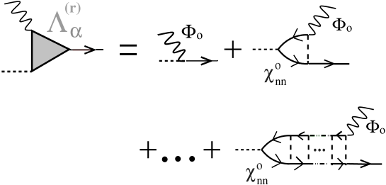
FIG. 2.: Diagrams contributing to $\Lambda^{(r)}_{\alpha}$.

FIG. 3.: Contributions to $\Sigma^{(r)}_{\alpha\beta}$.

FIG. 4.: Contributions to $\Sigma^{(r)}_{1}$.

FIG. 5.: The chemical potential $\mu$ of the condensed phase in units of $k_{B}T$ as a function of the condensate fraction $n_{c}/n$ for fixed temperature. The plot is made for the coupling strength $g=0.3\lambda_{\rm th}^{3}k_{B}T/\zeta(3/2)$. The horizontal long-dashed lines represent the borders of multi-stability, the upper one given by $\mu^{\rm(max)}=2g\lambda_{\rm th}^{-3}\zeta(3/2)$ the lower one $\mu^{\rm(min)}$ by the instability condition $g\chi(0,0)=-1/2$. The stable part of the curve is plotted as a solid line changing to a long-dashed line in the region of instability.

FIG. 6.: The chemical potential $\mu$ of the condensed and the uncondensed Bose gas in units of $k_{B}T$ as a function of the particle density $n$ in units of $\zeta(3/2)\lambda_{\rm th}^{-3}$ for the same value of the coupling constant $g$ as in Fig. 5. The long-dashed curve represents the unstable part of the branch of the condensed phase.

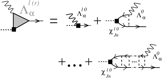
FIG. 7.: Diagrams contributing to $\Lambda^{l(r)}_{\alpha}$.
The symbol $\blacksquare$ denotes the longitudinal component of the gradient.

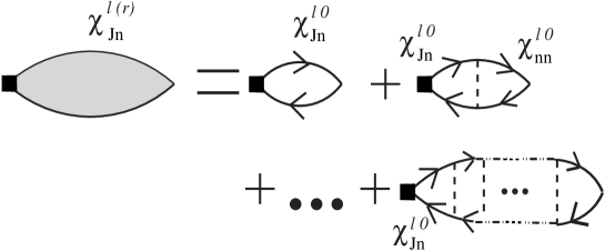
FIG. 8.: Regular current-density autocorrelation function $\chi^{l\,(r)}_{Jn}$ corresponding to $\chi^{(r)}_{\rm nn}$

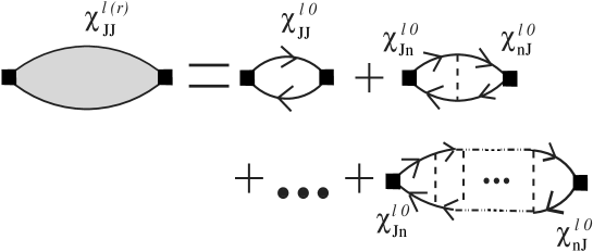
FIG. 9.: Regular current-current autocorrelation function $\chi^{l\,(r)}_{JJ}$ corresponding to $\chi^{(r)}_{\rm nn}$

FIG. 10.: Real part (left) and imaginary part (right) of the different branches of the velocity of sound $c=\omega/|\mathchoice{{\hbox{\boldmath$\displaystyle k$}}}{{\hbox{\boldmath$\textstyle k$}}}{{\hbox{\boldmath$\scriptstyle k$}}}{{\hbox{\boldmath$\scriptscriptstyle k$}}}|$ from (45) and (47) in units $\sqrt{k_{B}T_{c}/m}$ for the interaction $gn_{\rm tot}/k_{B}T_{c}=0.1$ depending on the temperature $T/T_{c}\,.$

FIG. 11.: Real part and imaginary part of the different branches of the velocity of sound $c$ in units $\sqrt{k_{B}T_{c}/m}$ for the interaction $gn_{\rm tot}/k_{B}T_{c}=0.3\,.$

REFERENCES

• [1] M. H. Anderson, J. R. Ensher, M. R. Matthews, C. E. Wieman, and E. A. Cornell, Science 269, 198 (1995); K. B. Davis, M.-O. Mewes, M. R. Andrews, N. J. van Druten, D. S. Durfee, D. M. Kurn, and W. Ketterle, Phys. Rev. Lett. 75, 3969 (1995); C. C. Bradley, C. A. Sackett, J. J. Tollett, and R. G. Hulet, Phys. Rev. Lett. 75, 1687 (1995); C. C. Bradley, C. A. Sackett, and R. G. Hulet, Phys. Rev. Lett. 78, 985 (1997).
• [2] W. Ketterle, D. S. Durfee, and D. M. Stamper-Kurn, in Bose-Einstein Condensation in Atomic Gases, Proceedings of the International School of Physics “Enrico Fermi”, ed. by M. I. Inguscio, S. Stringari, and C. E. Wieman (IOS Press, Amsterdam, 1999).
• [3] E. A. Cornell, J. R. Ensher and C. E. Wieman, in Ref. [2].
• [4] F. Dalvovo, S. Giorgini, L. Pitaevskii, and S. Stringari, Rev. Mod. Phys. 71, 463 (1999); K. Burnett, Contemp. Phys. 37, 1 (1996); A. S. Parkins and D. F. Walls, Phys. Rep. 303, 1 (1998).
• [5] D. S. Jin, J. R. Ensher, M. R. Matthews, C. E. Wiemann, and E. A. Cornell, Phys. Rev. Lett. 77, 420 (1996).
• [6] M.-O. Mewes, M. R. Andrews, N. J. van Druten, D. M. Kurn, D. S. Durfee, and W. Ketterle, Phys. Rev. Lett. 77, 416 (1996).
• [7] M. R. Andrews, D. M. Kurn, H.-J. Miesner, D. S. Durfee, C. G. Townsend, S. Inouye, and W. Ketterle, Phys. Rev. Lett. 79, 553 (1997).
• [8] P. C. Hohenberg and P.C. Martin, Ann. Phys. 34, 291 (1965).
• [9] V. K. Wong and H. Gould, Ann. Phys. (N. Y.) 83, 252 (1974).
• [10] D. Forster, Hydrodynamic fluctuations, broken symmetry, and correlation functions (Benjamin, Massachusetts, 1975).
• [11] J. Reidl, A. Csordás, R. Graham, P. Szépfalusy, Phys. Rev. A 61, 43606 (2000).
• [12] A. Griffin, Excitations in a Bose-Condensed Liquid (Cambridge University Press, Cambridge, 1993).
• [13] P. Szépfalusy and I. Kondor, Ann. Phys. (N.Y.) 82, 1 (1974).
• [14] D. S. Jin, M. R. Matthews, J.R. Ensher, C.E. Wieman, E.A. Cornell, Phys. Rev. Lett. 78, 764 (1997).
• [15] I. Kondor and P. Szépfalusy, Phys. Lett. 33A, 311 (1970).
• [16] S.-K. Ma, H. Gould, and V. K. Wong, Phys. Rev. A 3, 1453 (1971).
• [17] A. Griffin and T. H. Cheung, Phys. Rev. A 7, 2086 (1973).
• [18] E. Talbot and A. Griffin, Ann. Phys. 151, 71 (1983).
• [19] S. H. Payne and A. Griffin, Phys. Rev. B 32, 7199 (1985).
• [20] A. L. Fetter and J. D. Walecka, Quantum theory of many particle systems (McGraw Hill, New York, 1971).
• [21] S. T. Beliaev, Sov. Phys. JETP 7, 289 (1958); 7, 299 (1958).
• [22] H. Shi and A. Griffin, Phys. Rep. 304,1 (1998).
• [23] W. V. Liu, Phys. Rev. Lett. 79, 4056 (1997).
• [24] L. P. Pitaevskii and S. Stringari, Phys. Lett. A 235, 398, (1997).
• [25] P. O. Fedichev and G. V.  Shlyapnikov, Phys. Rev. A 58, 3146 (1998).
• [26] S. Giorgini, Phys. Rev. A 57 2949 (1998).
• [27] T. H. Cheung and A. Griffin, Phys. Rev. A 4, 237 (1971).
• [28] A. Minguzzi and M. P. Tosi, J. Phys. Condens. Matter 9, 10211 (1997).
• [29] K. Huang, C. N. Yang, and J. M. Luttinger, Phys. Rev. 105, 776 (1957).
• [30] V. N. Popov, Functional integrals and collective excitations (Cambridge University Press, Cambridge, 1987).
• [31] A. Griffin, Phys. Rev. B 53, 9341 (1996).
• [32] V. V. Goldman, I. F. Silvera, and A. J. Leggett, Phys. Rev. B 24, 2870 (1981).
• [33] D. A. Huse and E. D. Siggia, J. Low. Temp. Phys. 46, 137 (1982).
• [34] Y. Pomeau and S. Rica, J. Phys. A: Math. Gen. 33, 691, (2000).
• [35] S. Giorgini, Phys. Rev. A 61, 063615 (2000).
• [36] J. F. Dobson, Phys. Rev. Lett. 73, 2244 (1994).
• [37] G. Bene, J. Reidl, R. Graham and P. Szépfalusy, Phys. Rev. A (2001).
• [38] M. J. Bijlsma and H. Stoof, Phys. Rev. A 60, 3973 (1999).
• [39] U. Al Khawaja and H. Stoof, cond-mat/0003517
Refer to caption