KUCP0154
Pareto’s Law for Income of Individuals and Debt of Bankrupt Companies

Abstract

We analyze the distribution of income and income tax of individuals in Japan for the fiscal year 1998. From the rank-size plots we find that the accumulated probability distribution of both data obey a power law with a Pareto exponent very close to $-2$. We also present an analysis of the distribution of the debts owed by bankrupt companies from 1997 to March, 2000, which is consistent with a power law behavior with a Pareto exponent equal to $-1$. This power law is the same as that of the income distribution of companies. Possible implications of these findings for model building are discussed.

1 Introduction

More than a century ago the Italian sociologist Pareto studied the distribution of personal incomes for the purpose of characterizing a whole country’s economic status [1]. He found power law cumulative distributions with exponents close to $-1.5$ for several countries, which turned out to be a classic example of fractal distributions [2]. In 1922 Gini checked the same statistics and reported that power laws actually hold, but the values of the exponents vary from country to country [3]. Montroll and Shlesinger analyzed the USA’s personal income data for the year 1935–36 and found that the top 1% of incomes follow a power law with an exponent $-1.63$, while the rest, who are expected to be salaried, follow a log-normal distribution [4]. Although these results are interesting and suggestive, the data are all old, and a much more precise analysis using contemporary high quality data in digital form is desirable. One of this paper’s aims is to answer this requirement by showing the results of personal income distribution analysis on the latest high precision data reported to the tax office in Japan. As we will show in section 2 we find a clear power law with an exponent very close to $-2$, the first time it has been reported in this kind of study.

There is another topic in this paper that is related to personal incomes, but in a juridical sense, namely, company incomes. It was recently reported by Okuyama and Takayasu, who analyzed high quality Japanese company data for the year 1997, that the income distribution of companies accurately follows Zipf’s law, that is, a cumulative distribution with exponent $-1$ [5]. It is anticipated that this law holds rather universally for different years, for different countries, and even for each job category, with some exceptions. The second aim of this paper is to show a complementary result relating to the company income distributions, that is, the distribution of debts of bankrupt companies, which may correspond to the distribution of negative incomes. Although the data available for this purpose is limited we can apparently demonstrate that the debts distribution also follows the same statistics, Zipf’s law.

In the following section we give the details of our personal income distribution analysis. We briefly describe the result of the debt distribution in section 3, and the final section is devoted to discussions of the implications and significance of our results.

2 The income and income-tax distributions

The data we have for income and income tax are in many senses complementary. Both data relate to Japan, and the income data is for the fiscal year 1997 and 1998, while the income-tax data is only for 1998. For the fiscal year 1998, the income data contains all 6,224,254 workers who filed tax returns, but it is a coarsely tabulated data, while the income-tax data lists the income tax of individuals who paid tax of ten million yen or more in the same year. In this section we study the distribution of each data set and then combine them to obtain an over-all picture of income distribution in high income range.

The tabulated data for the income distribution of individuals in Japan is publicly available on the web pages of the Japanese Tax Administration [6]. Since the relevant pages are in Japanese only, we quote the data for the fiscal year 1998 in Table 1, where and hereafter we denote the income by $s$ in units of million yen. It should be noted that this data is for individuals who filed a tax return, and therefore does not include all individuals with income. Under the Japanese tax system, if a worker has only one source of income (salary) and the income is less than 20,000,000 yen, that person does not have to file a tax return (the tax deducted from the monthly salary is adjusted at the end of the year by the employer and that becomes the final amount of tax paid). In some circumstances, even if the income is below this amount, a person may have to file a tax return if some other conditions are met. Consequently, a large number of individuals in fact submit returns. Therefore for $s<20$ this data represents only a portion of the actual number of individuals, and we expect that the deviation between the number of people in this table and the actual number of people in that income range becomes larger in lower income ranges. Rigorously speaking, it is safe to trust only the entries for income $s\geq 20$ (the last three columns) in this data as a faithful representation of the number of individuals in that income range.

Income ($s$-million yen)	Number
$s\leq 0.7$	14,496
$0.7<s\leq 1$	73,352
$1<s\leq 1.5$	359,157
$1.5<s\leq 2$	541,739
$2<s\leq 2.5$	565,835
$2.5<s\leq 3$	584,989
$3<s\leq 4$	954,901
$4<s\leq 5$	687,057
$5<s\leq 6$	497,438
$6<s\leq 7$	375,485
$7<s\leq 8$	288,141
$8<s\leq 10$	379,716
$10<s\leq 12$	229,205
$12<s\leq 15$	215,712
$15<s\leq 20$	190,524
$20<s\leq 30$	140,533
$30<s\leq 50$	82,514
$50<s$	43,455

Table 1: The tabulated data of the income of 6,224,254 individuals in Japan in fiscal year 1998.

In Fig. 1 we give the rank-size plot, which is the log-log plot of the rank ($r$) as a function of income ($s$). The vertical axis may be converted to the accumulated probability $P(\geq s)$, the probability that a given individual has income equal to or greater than $s$. This is done by simple rescaling $P(\geq s)=r(s)/r(0)$ where $r(0)=6,224,254$, and therefore it merely induces a translation of the vertical axis in the log plot and does not change the shape of the distribution. The ticks for the accumulated probability $P(\geq s)$ are placed on the right-hand side of the plot. It is apparent that this plot tends to a linear function in the high income range, say $s>10^{1}$. As we have noted above, this distribution should be equal to that of all the workers only for $s\geq 20$. Therefore we have calculated the best-fit linear function from the last three data points and have found that it is given by the following;

$$r\propto s^{-1.98}.$$ (1)

The broken line in Fig.1 represents this function. The distribution $P(\geq s)$ fits the power law (1) very well in the high income range and it gradually deviates from (1) as the income becomes lower. Since this deviation starts to grow as the income $s$ becomes lower than 20, we may assume that the power law (1) applies to a much wider range of incomes.

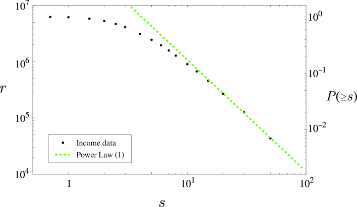
Figure 1: The rank-size plot of the income distribution of Table 1 (dots) and the linear approximation (broken line) given by Eq.(1).

Another set of publicly available data is a list of all taxpayers who paid income-tax of ten million yen or more in 1998. Hereafter we denote the tax by $t$ in million yen. There are 84,515 such individuals listed for fiscal year 1998. The rank-size plot of this data is given in Fig.2. This distribution is very close to being linear in this log-log plot. The best-fit result is given by the following;

$$r\propto t^{-2.05}.$$ (2)

This function is given by the dotted line in Fig.2.

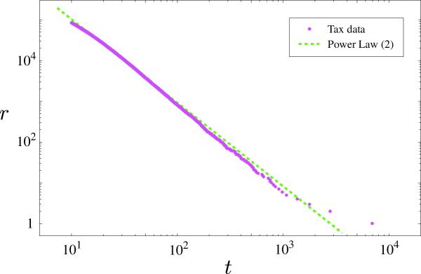
Figure 2: The rank-size plot of the income-tax listing (dots) and the function (2) obtained by the best-fit method (broken line).

The fact that the income-tax distribution satisfies Eq.(2), which is very close to the income distribution Eq.(1), implies that income-tax is roughly proportional to the income. This proportionality constant can be fixed by assuming that the income-tax is a monotonically increasing function of the income, which we expect to be true in an averaged sense. By this assumption a given person has the same rank in both the income listing and the income-tax listing. Therefore the relation between income and income-tax can be found in the overlapping region of those two data. The data of incomes, however, is given only in approximate form by Table 1, while the listing of the income-tax covers the bottom one and a half columns. Therefore, the comparison between the income and the income-tax is possible only for the rank $r=43,455$ whose income was $s=50$. From our listing of the income-tax we find that the 43,455th ranked person has paid income tax of $t=15.13$. Therefore we find that

$$t=0.30\,s.$$ (3)

In the fiscal year 1998, the tax ($t$) was obtained from the income ($s$) in three steps: (1) various deductions, such as the basic (default) deduction, deductions for the spouse and the dependents, and insurance deductions, were made to calculate the taxable income ($s^{\prime}$), (2) the basic tax ($t^{\prime}$) is calculated according to the formula $t^{\prime}=0.5s^{\prime}-6.03$ in this income range, and (3) further deductions, such as the deduction for donation to political parties, deduction for housing loans and further special deductions are made to arrive at the actual tax $t$. Although it is difficult to assess the validity of the result (3), it may be understood as an averaged result of these steps, especially since the proportionality constant is meaningfully less than the constant 0.5 of the tax formula.

Using the result (3), we translate the income-tax data to the income data. This way, the shortcoming of the original income data, that it lacks the information in the high income range, can be overcome. The resulting rank-size plot is given in Fig.3.

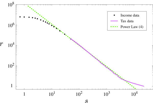
Figure 3: The rank-size plot of the income. The data in Table 1 is shown by dots as in Fig.1, whereas the data points induced from the income-tax listing by Eq.(3) are connected by the solid line-segments. The broken line shows the function (4) obtained by the best-fit method.

Again, the power-law behavior is apparent in Fig.3. Caution is needed in applying the best-fit method; The data points of the tax-induced income becomes very dense at lower $s$, therefore they would dominate the result if all data points are treated with equal weight in a simple best-fit method. The data of original income table would certainly be neglected in such an analysis. For this reason, we have calculated the best fit to the power law from each of the two columns in Table 1 and each of the five sections $[50\times 2^{n},50\times 2^{n+1}](n=1\cdots 5)$ of the tax-induced income data and have taken the average of the seven linear functions (in the log-log scale). The result is the following;

$$r\propto s^{-2.06}.$$ (4)

The broken line in Fig.3 denotes this function. We find that the power-law (4) fits the data over three magnitude of income, $10<S<10^{4}$.

As mentioned earlier, the deviation of the income data points from the power law in the range $s<20$ may be explained as the result of the exclusion of the majority of the workers of single salary source. On the other hand, there is a possibility that the distribution in the lower ranges follow the log-normal distribution as was suggested by Montroll and Shlesinger [4]. Therefore it is highly desirable to investigate these lower ranges of income to obtain the overall profile of the income distribution. One such study toward this direction is currently in progress by one of the authors (W.S.) and will be published in near future [7].

3 Debts of bankrupt companies

The data we have gathered covers some 100 big bankruptcies in Japan from 1997 to the end of March, 2000. Unfortunately the exact criteria for the choice of the “big” cases is not known. The resulting rank-size plot for the accumulated probability $P(\geq d)$ is given in Fig.4, where we have denoted the debt in units of million yen by $d$. The data actually contains much smaller cases, but from the fact that the number of data starts to decrease for $d<10^{5}$ we assume that the data starts to loose reliability in this range. The broken line represents the Zipf law,

$$r\propto d^{-1},$$ (5)

which were found for the company income previously [5]. This data is in reasonable agreement with this power-law.

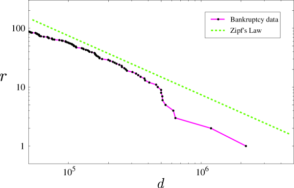
Figure 4: The rank-size plot of the accumulated probability $P(\geq d)$ of the debt ($d$) from 1997 to March, 2000. The broken line is the Zipf law (5) shown for visual reference.

4 Discussion

As described in section 2 we have discovered a new type of income distribution for individuals, the power law distribution with an exponent close to $-2.0$. If we assume that all the pioneering results together with our result, then the only consistent interpretation may be as follows: Income distribution generally follows a power law for large incomes but its exponent varies from country to country and year to year. As noted, Pareto and Gini give different exponents using data from different years. However, there is a possibility that such old results may based on imperfect data, and we may still expect a kind of universal behavior for personal income distributions. In our analysis the observed scale range satisfying the power law in Fig.3 is about three decades in the income rank range ($10$ to $10^{4}$), therefore, the estimation of the exponent is quite accurate. We need comparably high precision data for other countries or years for further discussion about such universality.

There has been no established theory for the income distributions. A classical theory was proposed by Gibrat in 1932 [8]. He assumed the time evolution of each person’s income to be approximated by a multiplicative stochastic process considering that a random process proportional to the amount of the present income can approximate the increase and decrease of income. By this assumption the resulting distribution of income follows a log-normal distribution which is consistent with the result of Montroll and Shlesinger for salaried people. However, this theory apparently fails to explain the more interesting part of the distribution, the power law tails.

Explaining the existence of power law tails with the level of simplicity in Gibrat’s theory can easily be done as follows by introducing a simple modification to his model. Let us introduce an additive random term together with the multiplicative term, such as

$$I(t+1)=a(t)I(t)+R(t).$$ (6)

If we assume that $a(t)$ and $R(t)$ are independent random variables then it is mathematically shown that the distribution of $I(t)$ follows a general power law even in a case where the fluctuation of $a(t)$ is correlated [9]. In the simplest case when both $a(t)$ and $R(t)$ are white noises, the power law exponent, $\beta$, of the distribution of $I(t)$ is simply given by the following formula [10],

$$\langle a^{\beta}\rangle=1.$$ (7)

Based on this relation the power law distribution with an anticipated exponent can be obtained by only tuning the statistics of growth rate, $a(t)$.

There can be many different approaches other than this simple growth model. One straightforward model can be given by relating the company’s incomes to personal incomes by assuming that the high income individuals are mostly company owners. If we can assume that company owner’s income is proportional to the square root of the company’s income, then the established empirical Zipf’s law for the company’s income reduces the squared power law for individuals.

Nonlinear interaction models of incomes may also be important such as the model introduced by Levy and Solomon [13]. An obvious difficulty in such modeling is the mathematical form of interaction among people working in real economics. For example economical interaction such as buying and selling generally occur in a discrete manner both in time and price, therefore, it is even problematic whether we can introduce an analytical function as an interaction term.

Related to the issue of the income distribution and the dynamics behind it is the distribution of wealth of individuals. One such data set, from the Forbes 400, is analyzed in Ref.[14], and is shown to have the Pareto exponent close to $-1.36$. We have recently carried out a similar analysis with 1996–1999 data of approximately 400 of the richest people of U.S.A. and 100 of the richest people in Japan and found that the results are consistent with this exponent.

As there is no steady model of personal incomes it is important to approach from many different aspects. Personal income might be related to a kind of popularity such as the citation numbers in scientific publications or access number distribution for Internet homepages. Citation frequency distribution has been examined for publications in the field of physics and a power law tail with exponent about $-3$ is reported [11]. As for homepage popularity ranking it is known that we have another Zipf’s law for this quantity, namely the power law exponent is about $-1$ [12].

Our other finding concerning the distribution of bankrupt companies is considered to be suggestive for the understanding of money flow statistics among companies. The amount of debt of a company is roughly given by accumulated negative incomes that exceeded the whole asset of the company. Therefore, combining our result with the known Zipf’s law for positive incomes we may conjecture that the distributions of money flows among companies both positive and negative generally tend to follow Zipf’s law.

For the purpose of construction of a numerical model of company income statistics, we can summarize the known conditions to be satisfied as follows:

1. The amount of annual summation of outgoing money from each company is of the same order of its assets, also the summation of incoming money is of the same order of the assets [5].

2. By definition a company’s income is given by the difference of these moneys, that is, incoming money minus outgoing money. The averaged incomes is nearly proportional to a fractional power of asset with exponent estimated to be about 0.85 [5].

3. The distribution of income follows Zipf’s law for both positive and negative regions.

4. The variance of growth fluctuation of assets is proportional to a fractional power of assets with exponent about $-0.15$ [15].

5. The distribution of assets seems to follow a log-normal law [16], but we need better quality real data to assess this empirical law.

Although no model has successfully satisfied all of these conditions, there are two promising approaches towards this goal. One is a company interaction model based on a zero-sum game [10] introduced to explain the asset’s variance law 4. In this model companies play a kind of stochastic game in which money flow from losers to winners according to a certain rule. In this model the condition 4 and 5 are satisfied in a rough sense, however, condition 3 is not fulfilled. The condition 1 depends on the definition of the annual year, which can be tuned, while condition 2 has not been checked.

The other approach is a territory occupation model that is based on the assumption that a company’s income may be proportional to the share of customers [17]. Companies under certain stochastic rules in this model share the customers in a new field of a market. From this approach it is easy to satisfy Zipf’s law for positive incomes. However, other conditions are out of the range at present.

Acknowledgments
The authors would like to thank Mr. Nakano of the Japanese Tax Administration for conversation on the properties of the data on the web pages. Numerical computation in this work was in part supported by the computing facility at the Yukawa Institute for Theoretical Physics. The authors would also like to thank Dr. John Constable (Magdalene College, U.K.) for careful reading of the manuscript.

References

- [1] V. Pareto, Le Cours d’Économie Politique (Macmillan, London, 1897).
- [2] B. P. Mandelbrot, The Fractal Geometry of Nature, (Freeman, San Francisco, 1982).
- [3] C. Gini, Indici di concentrazione e di dipendenza, Biblioteca delli’ecoomista 20 (1922).
- [4] E. W. Montroll and M. F. Shlesinger, J. Stat. Phys. 32, 209 (1983).
- [5] K. Okuyama, M. Takayasu and H. Takayasu, Physica A 269, 125 (1999).
- [6] The Japanese Tax Administration, http://www.nta.go.jp.
- [7] W. Souma, in preparation.
- [8] R. Gibrat, Les inégalitś économiques (Paris, Sirey).
- [9] A.-H. Sato and H. Takayasu, Physica A250, 231 (1997).
- [10] H. Takayasu, A.-H. Sato, and M. Takayasu, Phys. Rev. Lett. 79, 966 (1997).
- [11] S. Redner, Eur. Phys. J. B4, 131 (1998).
- [12] J. Nielsen, http://www.useit.com/alertbox/zipf.html
- [13] M. Levy and S. Solomon, Int. J. Mod. Phys. C7, 595 (1996).
- [14] M. Levy and S. Solomon, Physica A242, 90 (1997).
- [15] H. H. R. Stanley, L. A. N. Amaral, S. V. Buldyrev, S. Havline, H. Leschhorn, P. Maass, M. A. Salinger and H. E. Stanley, Nature 379, 804 (1996).
- [16] L. A. N. Amaral, S. V. Buldyrev, S. Havlin, M. A. Salinger, and H. E. Stanley, Phys. Rev. Lett. 80, 1385 (1998).
- [17] H. Takayasu, M. Takayasu, M. P. Okazaki, K. Marumo and T. Shimizu, Paradigms of Complexity, p.243 (ed. M. M. Novak, World Scientific, Singapore, 2000).