Magnetization plateaus of the Shastry-Sutherland model for SrCu₂(BO₃)₂: Spin-density wave, supersolid and bound states

Abstract

We study the Heisenberg antiferromagnet on the Shastry-Sutherland lattice under magnetic fields, to clarify the magnetic properties of SrCu₂(BO₃)₂. Treating magnetic excitations promoted by the field as Bose particles and using strong coupling expansion, we derive an effective Hamiltonian for the effective magnetic particles. Anisotropic repulsive interactions between effective particles induce ‘insulating’ states with a stripe SDW structure at magnetization $m/m_{\rm sat}=1/3$ and a checkerboard structure at 1/2, and thereby form magnetization plateaus. Supersolid phases appear around insulating SDW phases by changing the magnetic field. Nature of these supersolid phases is discussed in detail. We also demonstrate how the geometry of the Shastry-Sutherland lattice affects dynamical properties of magnetic excitations significantly and makes a novel type of quintuplet ($S=2$) boundstates condense for very small magnetization.

]

I Introduction

Since plateau structures were observed in the magnetization process of a series of quasi one-dimensional Ni-compounds[2], magnetization plateaus have been attracting extensive interests. The appearance of plateaus in magnetization curves was explained as metal-insulator transitions of magnetic excitations driven by a magnetic field[3]; Magnetic excitations crystallize and form SDW in the plateau states, and they are itinerant in the non-plateau states. Recently it was discussed that this phenomenon is not limited to the one-dimensional systems, but more general, and occurs in two- and three-dimensional systems as well[4, 5, 6]. Before the recent studies, magnetization plateaus were already known to appear at $m/m_{\rm sat}=1/3$ in the antiferromagnetic compounds on the triangular lattice, C₆Eu[7], CsCuCl₃[8], and RbFe(MoO₄)₂[9]. Theoretically, plateaus were seen at $m/m_{\rm sat}=1/3$ in the Heisenberg antiferromagnet on the triangular lattice[10, 11, 12], and also at $m/m_{\rm sat}=1/2$ in the multiple-spin exchange model with four-spin interactions[13, 5]. The 1/3-plateau comes from appearance of a collinear uud state[10, 11, 12] and the 1/2-plateau from the uuud state[13, 5]. These magnetization plateaus can also be regarded as superfluid-insulator transitions of flipped-spin degree of freedom[5, 6]. It may be worth mentioning that there is also another trial to realize magnetization plateau in two-dimensional systems as gapped spin liquid states analogous to the FQHE wave functions[14].

Recently a quasi two-dimensional compound SrCu₂(BO₃)₂ is attracting extensive interests because it shows magnetization plateaus and peculiar dynamical properties. The two-dimensional lattice structure of Cu²⁺ ions in SrCu₂(BO₃)₂ is the so-called Shastry-Sutherland lattice[15, 16], which is shown in Fig. 1. Susceptibility and specific heat data show that interactions are antiferromagnetic, the spin excitation has a gap above the ground state, and the spin anisotropy is weak[16]. This material seems[17] to be well described with the $S=1/2$ Heisenberg antiferromagnet on the Shastry-Sutherland lattice[18]. (Hereafter we call this model simply as Shastry-Sutherland model.) The ground state of the Shastry-Sutherland model is exactly a direct product of local dimer singlets on bonds $J$ for the region $J^{\prime}/J<0.68$ (Refs. [18, 17]) and there is a finite gap above the ground state. Susceptibility and specific heat estimated from this model with $J^{\prime}/J=0.68$ fit well with the experimental results[17]. (Recently the value has been modified to $J^{\prime}/J=0.635$ by taking into account the three-dimensional coupling of Shastry-Sutherland layers.[19]) In ref. [16], Kageyama et al. reported two plateaus at $m/m_{\rm sat}=1/8$ and $1/4$ in the magnetization curve of SrCu₂(BO₃)₂. Theoretically, we studied the magnetization process of the Shastry-Sutherland model, treating a dimer triplet as a particle, and thereby predicted a novel broad plateau at $m/m_{\rm sat}=1/3$ in the previous report[6]. It was argued that the appearance is due to superfluid-insulator transition of the excitations. Quite recently, the above 1/3-plateau was experimentally observed in magnetization measurements up to a strong field of 57[T][20]. As was predicted in ref. [6], this plateau is the broadest one ever found in this material. This seems to support the correctness of our argument based on the particle picture. This material also shows peculiar dynamical properties[21, 22, 23, 24], e.g. one-magnon excitation is almost dispersionless, but two-magnon excitations have strong dispersion[21]. The aim of this paper is to present the details of our analyses and results reported briefly in ref. [6], and to proceed further thereby giving remarkable consequences of the correlating hopping of the effective Hamiltonian. This correlated hopping can also explain the peculiar dynamical behaviors observed in experiments[25].

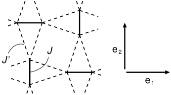
FIG. 1.: Shastry-Sutherland lattice. Solid (dotted) lines denote bonds with strong exchange $J$ (weak one $J^{\prime}$).

The ground state of the Shastry-Sutherland model at zero magnetic field was studied for a varying ratio $J^{\prime}/J$ by the mean field approximation[26], exact diagonalization method[17], and series expansion[27]. It was found[27] that the ground state is the exact dimer state for $J^{\prime}/J<0.69$, a gapped plaquette singlet state for $0.69<J^{\prime}/J<0.86$, and Néel-ordered state for $0.86<J^{\prime}/J$. The parameters of SrCu₂(BO₃)₂ estimated[17, 19] as $J^{\prime}/J=0.68$ (or 0.635) suggest that the spin state of the real material belongs to the dimer phase, but it is very close to the phase boundary with the plaquette singlet phase. Consistency between theoretical and experimental results on magnetization plateau at $m/m_{\rm sat}=1/3$[6, 20] and dynamical behavior in inelastic neutron scattering[21, 25] also supports that the real material is in the dimer phase.

In this paper, we study the $S=1/2$ Heisenberg antiferromagnet on the Shastry-Sutherland lattice and discuss the magnetic properties under a magnetic field. We analyze this model using strong-coupling expansion. In section II, we derive an effective Hamiltonian for the dimer-triplet excitations. Virtual triplet excitations yield various effective repulsive interactions, which are responsible for the plateaus. Although the usual single-particle hopping is completely missing from the resulting Hamiltonian, correlated hopping processes are contained instead.

In section III, we investigate the magnetization process applying the classical approximation to the effective (pseudo-spin) Hamiltonian and show that plateaus appear at $m/m_{\rm sat}=1/3$ and $1/2$. Both of the plateau states are Mott (SDW) insulators of magnetic excitations. Spatially anisotropic interactions perturbatively generated stabilize several SDW structures. Near the plateau states, there are supersolid phases, in which SDW long-range order (LRO) and superfluid coexist[29, 30, 31, 32, 33]. Field ($B$) versus coupling ($J^{\prime}/J$) phase diagram is also presented.

Although the inter-dimer coupling $J^{\prime}/J$ is not small, the special geometry of the Shastry-Sutherland lattice strongly suppresses bare one-particle hopping and hence the correlated hopping becomes important. This fact leads to remarkable consequences on the motion of magnetic excitations. In section IV, we investigate correlated hopping more closely and demonstrate how it favors the formation of a bound pair of dimer triplets which repel each other at the level of the bare Hamiltonian. This bound state has a relatively large dispersion and may be an elementary particle at very low magnetization, instead of the single dimer triplet. The non-plateau state would be superfluid of these bound states at least for very small magnetization. Above a certain threshold value of magnetization, individual dimer triplets become elementary particles and the non-plateau state is characterized by superfluidity of single dimer triplets.

In section V, we also discuss spin excitation just below the saturation field. It is found that lowest energy states exist on a close curve instead of a point in the momentum space.

Critical phenomena of the plateau transition are discussed in section VI and are argued to be in the same universality class as the superfluid transition of the interacting boson system in the dilute limit.

II Effective Hamiltonian

In this section we derive an effective Hamiltonian for the magnetic excitations under a strong enough magnetic field. We begin with the $J^{\prime}=0$ limit. In this limit, the lowest triplet excitation over the (dimer) singlet ground state is apparently obtained by promoting one of the dimer singlets to a triplet. Although the dimer product remains to be the exact ground state even for non-zero $J^{\prime}$, the above completely localized triplet does not; perturbation $J^{\prime}$ ‘broadens’ the triplet by exciting nearby singlets. Unlike the ground state which is perfectly free from quantum fluctuation, excited states strongly suffer from it. This is one of the most important features of the model. As a result, (physical) triplets can interact with each other with the help of virtual triplets created by perturbation and the effective Hamiltonian for the physical triplet degrees of freedom should contain effective interactions.

The most systematic way to take into account such virtual processes would be the strong-coupling expansion[3, 4]. We start from the limit $J^{\prime}=0$ and treat the interaction with coupling $J^{\prime}$ by perturbation. In the absence of the external field, the spin states of a single isolated dimer ($J$) bond consists of a singlet and triplet separated by a gap $J$. When the field is increased until the lowest triplet with $S^{z}=1$ intersects the singlet, we may keep only two states–the singlet and the lowest triplet–as the physical degrees of freedom as far as the low-energy sector is considered.

We carry out the degenerate perturbation for such low-energy degrees of freedom. Considering the triplet ($S=1$) state with $S^{z}=1$ as a particle (a hard-core boson) and the dimer singlet ($S=0$) as a vacancy, we derive an effective Hamiltonian for the magnetic particles. (Rest of spin states, i.e. triplets with $S^{z}=0$ and $-1$, are included into the intermediate virtual states of the perturbation.) The perturbational expansion is performed up to the 3rd order in $J^{\prime}/J$ for degenerate states with a constant number of dimer triplet excitations with $S^{z}=1$. The final form of the effective Hamiltonian is as follows

$$H = H_{0}+H_{1}+H_{2}+H_{3},$$ (1)

$$H_{0} = (J-B)\sum_{i}n_{i},$$ (2)

$$H_{1} = \frac{\displaystyle{J^{\prime}}}{\displaystyle{2}}\sum_{\langle i,j\rangle}n_{i}n_{j},$$ (3)

$$H_{2} = -\frac{\displaystyle{J^{\prime 2}}}{\displaystyle{J}}\sum_{i}n_{i}+\frac{\displaystyle{J^{\prime 2}}}{\displaystyle{2J}}\sum_{\langle i,j\rangle}n_{i}n_{j}$$ (4)

$$+ \frac{\displaystyle{J^{\prime 2}}}{\displaystyle{4J}}\sum_{i\in A}\{2n_{i+\mbox{\bf e}1}(1-n_{i})n_{i-\mbox{\bf e}1}+(b_{i+\mbox{\bf e}2}^{\dagger}b_{i-\mbox{\bf e}2}+h.c.)n_{i}$$ (6)

$$+(b_{i}^{\dagger}b_{i+\mbox{\bf e}2}-b_{i}^{\dagger}b_{i-\mbox{\bf e}2}+h.c.)(n_{i-\mbox{\bf e}1}-n_{i+\mbox{\bf e}1})\}$$

$$+ \frac{\displaystyle{J^{\prime 2}}}{\displaystyle{4J}}\sum_{i\in B}\{\ \ \ \mbox{\bf e}_{1}\leftrightarrow\mbox{\bf e}_{2}\ \ \ \},$$ (7)

$$H_{3} = -\frac{\displaystyle{J^{\prime 3}}}{\displaystyle{2J^{2}}}\sum_{i}n_{i}-\frac{\displaystyle{J^{\prime 3}}}{\displaystyle{8J^{2}}}\sum_{\rm NN}n_{i}n_{j}+\frac{\displaystyle{J^{\prime 3}}}{\displaystyle{4J^{2}}}\sum_{\rm NNN}n_{i}n_{j}$$ (8)

$$+ \frac{\displaystyle{J^{\prime 3}}}{\displaystyle{16J^{2}}}\sum_{i\in A}[4n_{i+\mbox{\bf e}2}n_{i}n_{i-\mbox{\bf e}2}-12n_{i+\mbox{\bf e}1}(n_{i}-1)n_{i-\mbox{\bf e}1}$$ (32)

$$+6(b_{i+\mbox{\bf e}2}^{\dagger}b_{i-\mbox{\bf e}2}+h.c.)n_{i}$$

$$+5(b_{i}^{\dagger}b_{i+\mbox{\bf e}2}-b_{i}^{\dagger}b_{i-\mbox{\bf e}2}+h.c.)(n_{i-\mbox{\bf e}1}-n_{i+\mbox{\bf e}1})$$

$$-(b_{i+\mbox{\bf e}2}^{\dagger}b_{i}+h.c.)(n_{i+\mbox{\bf e}2+\mbox{\bf e}1}n_{i-\mbox{\bf e}1}-n_{i+\mbox{\bf e}2-\mbox{\bf e}1}n_{i+\mbox{\bf e}1})$$

$$-(b_{i-\mbox{\bf e}2}^{\dagger}b_{i}+h.c.)(n_{i-\mbox{\bf e}2-\mbox{\bf e}1}n_{i+\mbox{\bf e}1}-n_{i-\mbox{\bf e}2+\mbox{\bf e}1}n_{i-\mbox{\bf e}1})$$

$$-2(b_{i+\mbox{\bf e}2+\mbox{\bf e}1}^{\dagger}b_{i}+h.c.)n_{i+\mbox{\bf e}2}n_{i-\mbox{\bf e}1}$$

$$-2(b_{i-\mbox{\bf e}2-\mbox{\bf e}1}^{\dagger}b_{i}+h.c.)n_{i-\mbox{\bf e}2}n_{i+\mbox{\bf e}1}$$

$$-2(b_{i-\mbox{\bf e}2+\mbox{\bf e}1}^{\dagger}b_{i}+h.c.)n_{i-\mbox{\bf e}2}n_{i-\mbox{\bf e}1}$$

$$-2(b_{i+\mbox{\bf e}2-\mbox{\bf e}1}^{\dagger}b_{i}+h.c.)n_{i+\mbox{\bf e}2}n_{i+\mbox{\bf e}1}$$

$$+(b_{i+\mbox{\bf e}2}^{\dagger}b_{i}+h.c.)(n_{i+\mbox{\bf e}2+\mbox{\bf e}1}n_{i+\mbox{\bf e}1}-n_{i+\mbox{\bf e}2-\mbox{\bf e}1}n_{i-\mbox{\bf e}1})$$

$$+(b_{i-\mbox{\bf e}2}^{\dagger}b_{i}+h.c.)(n_{i-\mbox{\bf e}2-\mbox{\bf e}1}n_{i-\mbox{\bf e}1}-n_{i-\mbox{\bf e}2+\mbox{\bf e}1}n_{i+\mbox{\bf e}1})$$

$$+2(b_{i+\mbox{\bf e}2+\mbox{\bf e}1}^{\dagger}b_{i}+h.c.)n_{i+\mbox{\bf e}2}n_{i+\mbox{\bf e}1}$$

$$+2(b_{i-\mbox{\bf e}2-\mbox{\bf e}1}^{\dagger}b_{i}+h.c.)n_{i-\mbox{\bf e}2}n_{i-\mbox{\bf e}1}$$

$$+2(b_{i-\mbox{\bf e}2+\mbox{\bf e}1}^{\dagger}b_{i}+h.c.)n_{i-\mbox{\bf e}2}n_{i+\mbox{\bf e}1}$$

$$+2(b_{i+\mbox{\bf e}2-\mbox{\bf e}1}^{\dagger}b_{i}+h.c.)n_{i+\mbox{\bf e}2}n_{i-\mbox{\bf e}1}$$

$$+2(b_{i+\mbox{\bf e}2-\mbox{\bf e}1}^{\dagger}b_{i-\mbox{\bf e}2}-b_{i+\mbox{\bf e}2+\mbox{\bf e}1}^{\dagger}b_{i-\mbox{\bf e}2}+h.c.)n_{i+\mbox{\bf e}2}n_{i}$$

$$+2(b_{i-\mbox{\bf e}2-\mbox{\bf e}1}^{\dagger}b_{i+\mbox{\bf e}2}-b_{i-\mbox{\bf e}2+\mbox{\bf e}1}^{\dagger}b_{i+\mbox{\bf e}2}+h.c.)n_{i-\mbox{\bf e}2}n_{i}$$

$$-(b_{i+\mbox{\bf e}2}^{\dagger}b_{i-\mbox{\bf e}2}+h.c.)n_{i}$$

$$\mbox{\hskip 14.22636pt}\times(n_{i+\mbox{\bf e}2+\mbox{\bf e}1}+n_{i+\mbox{\bf e}2-\mbox{\bf e}1}+n_{i-\mbox{\bf e}2-\mbox{\bf e}1}+n_{i-\mbox{\bf e}2+\mbox{\bf e}1})$$

$$-\{(b_{i}^{\dagger}b_{i-\mbox{\bf e}2}+h.c.)n_{i+\mbox{\bf e}2}-(b_{i}^{\dagger}b_{i+\mbox{\bf e}2}+h.c.)n_{i-\mbox{\bf e}2}\}$$

$$\mbox{\hskip 28.45274pt}\times(n_{i-\mbox{\bf e}1}-n_{i+\mbox{\bf e}1})$$

$$+2(b_{i+\mbox{\bf e}2}^{\dagger}b_{i-\mbox{\bf e}2}+h.c.)n_{i}(n_{i-\mbox{\bf e}1}+n_{i+\mbox{\bf e}1})$$

$$-3(b_{i}^{\dagger}b_{i-\mbox{\bf e}1}+h.c.)n_{i+\mbox{\bf e}1}(n_{i-\mbox{\bf e}2-\mbox{\bf e}1}-n_{i+\mbox{\bf e}2-\mbox{\bf e}1})$$

$$-3(b_{i}^{\dagger}b_{i+\mbox{\bf e}1}+h.c.)n_{i-\mbox{\bf e}1}(n_{i+\mbox{\bf e}2+\mbox{\bf e}1}-n_{i-\mbox{\bf e}2+\mbox{\bf e}1})]$$

$$+ \frac{\displaystyle{J^{\prime 3}}}{\displaystyle{16J^{2}}}\sum_{i\in B}[\ \ \ \mbox{\bf e}_{1}\leftrightarrow\mbox{\bf e}_{2}\ \ \ ],$$ (33)

where indices $i$ and $j$ run over an effective square lattice of dimer bonds (both horizontal and vertical), and $A$ ($B$) sublattice contains horizontal (vertical) ones. The operator $b^{\dagger}_{i}$ ($b_{i}$) creates (annihilates) magnetic particle with spin $S^{z}=1$ at bond $i$, and $n_{i}=b_{i}^{\dagger}b_{i}$. The unit vectors $\mbox{\bf e}_{1}$ and $\mbox{\bf e}_{2}$ are shown in Fig. 1. The interactions summed up on B sublattices are obtained by replacing $\mbox{\bf e}_{1}$ and $\mbox{\bf e}_{2}$ in those on A sublattices. The abbreviations NN and NNN denote pairs of nearest neighbor and next nearest neighbor sites.

The Hamiltonian derived above does not have the bare one-particle hopping terms like $b^{\dagger}_{i}b_{j}+b^{\dagger}_{j}b_{i}$, which means a single dimer triplet excitation is dispersionless at this order. This is in a striking contrast with other spin gap systems e.g. the 2-leg ladder. The energy gap of one dimer triplet excitation is evaluated as $\Delta E_{1}(B)=J-B-J^{\prime 2}/J-J^{\prime 3}/(2J^{2})$.

On the other hand, the effective Hamiltonian contains many correlated-hopping processes, where an effective hopping of a particle is mediated by another one. Roughly speaking, these are closely related to 2-particle Green functions of the triplet bosons. This correlated hopping is important for dynamics of the Shastry-Sutherland model and it leads to many interesting conclusions; bound states without attraction, supersolid with stripe structure, etc. Most terms of higher orders concern the correlated hopping.

Many two-body repulsive interactions are also derived, whose range and geometry are shown in Fig. 4 of Ref. [6]. The nearest neighbor repulsion $V_{\rm NN}$ and the next-nearest-neighbor one $V_{\rm NNN}$ are derived as $V_{\rm NN}=J^{\prime}/2+J^{\prime 2}/2J-J^{\prime 3}/8J^{2}$ and $V_{\rm NNN}=J^{\prime 3}/4J^{2}$. (There were a typographical error and a mistake in the coefficients of the 3rd order terms of $V_{\rm NN}$ and $V_{\rm NNN}$ in ref. [6]. There was also the same mistake in ref. [28].) The 3rd-neighbor repulsion $V_{\rm 3rd}$ between vertical (horizontal) bonds with the distance $2\mbox{\bf e}_{1}$ ($2\mbox{\bf e}_{2}$) is $V_{\rm 3rd}=J^{\prime 2}/2J+3J^{\prime 3}/4J^{2}$. Thus $V_{\rm 3rd}$ is anisotropic and acts only in one direction. The effective Hamiltonian (1) correctly reflects the space-group symmetry of the original Shastry-Sutherland model. If it is considered as a model of interacting hard-core bosons on a square lattice consisting of dimer bonds, it still contains matrix elements which are not invariant under naive $90^{\circ}$ rotation about one site. We show in section III that they lead to anisotropic SDW states with a stripe structure. Longer-range repulsions between particles can appear from higher-order perturbations. Actually, Miyahara and Ueda [28] independently took into account such long-range interactions in a phenomenological manner, also adding weak one-body hopping by hand. Our finding is that there is much stronger correlated hopping processes and that triplets are not necessarily localized.

III Magnetization process

In order to discuss the ground state properties of the effective Hamiltonian (1), we first consider only repulsive interactions. From naive consideration of the range and geometry of the repulsive interactions (see Fig. 4 in Ref. [6]), we can imagine various insulating density-wave states of dimer triplets. Let us treat the repulsive interactions obtained at different orders of $J^{\prime}/J$, separately.

• The strongest interaction comes from the 1st-order term and it is repulsive for adjacent triplets. This repulsive interaction chooses SDW with 2-(dimer)sublattices checkerboard structure at $m/m_{\rm sat}=1/2$, where the unit cell has 4 sites in the original Shastry-Sutherland lattice. (See Fig. 6(b) in Ref. [6].)

• The next strong repulsive interactions originate from 2nd order terms and they are contained in $V_{\rm NN}$ and $V_{\rm NNN}$. Because of anisotropic interaction $V_{\rm 3rd}$, a stripe SDW state with a 6-(dimer)sublattice structure is stabilized at $m/m_{\rm sat}=1/3$ as shown in Fig. 4.

• The 3rd-order perturbation generates the weakest interactions, which favor SDW of 10-(dimer)sublattices checkerboard structure at $m/m_{\rm sat}=1/5$.

These SDW states do not necessarily appear if we consider all interactions and correlated hopping terms together. Whether SDW insulator is realized or not is determined by competition between repulsive interactions and correlated hopping.

To consider both effects of correlated hoppings and interactions together, we study the effective Hamiltonian in the classical limit. To this end, we map the hard-core boson system to the $S=1/2$ quantum (pseudo)spin system and then approximate the Pauli matrices by the components of a classical unit vector. Within the mean-field approximation, we first search for the ground state taking into account two and four (dimer)sublattices with a checkerboard structure and also three (dimer)sublattices with a stripe structure, because insulating states with these configurations are expected from the above consideration. To take account of larger sublattice structures, we next study the ground state of a finite system with a Monte Carlo method, where we gradually decrease temperatures to zero. We consider a finite cluster of 60 dimers and impose a periodic boundary condition that matches with all SDW configurations expected from the repulsive interactions, i.e. 2-(dimer)sublattice and 5-(dimer)sublattice checkerboard structures and 3-(dimer)sublattice stripe one.

The evaluated magnetization processes are shown for the cases $J/J^{\prime}=0.45$, $0.6$, and $0.68$ in Figs. 2(a), (b), and (c), respectively. Plateau structures appear at magnetization $m/m_{\rm sat}=1/3$ and 1/2, but no plateau appears at $m/m_{\rm sat}=1/5$ and 1/4. Near $m/m_{\rm sat}=1/4$, the slope of the curve becomes less steep, but not flat. This means that the $m/m_{\rm sat}=1/4$ state is energetically stable, though it does not have spin gap. In the plateau phases at $m/m_{\rm sat}=1/3$ and 1/2, there are SDW orders and no off-diagonal long-range order (ODLRO), that is, collinear spin states are realized. In the non-plateau phases, spins have ODLRO. Spin configuration of each phase is explained in the following subsections. A remark is in order here about our classical approximation. We obtained several plateaus by analyzing the classical pseudo-spin Hamiltonian. From this, one may conclude that these plateaus are of a classical origin. However, the spins approximated by vectors are not the original ones but are pseudo spins obtained for quantum objects–spin singlet and triplet–and these plateaus are not classical.

FIG. 2.: Magnetization processes of the Shastry-Sutherland model with $J^{\prime}/J=0.45$ (a), $J^{\prime}/J=0.6$ (b), and $J^{\prime}/J=0.68$ (c). Solid line is obtained from the effective Hamiltonian in the classical limit and dotted one from the exact diagonalization (ED) of the original Shastry-Sutherland model with the size $N=24$. The solid line for $J^{\prime}/J=0.68$ (c), taken from Fig. 5 of Ref. [6], is also shown for the comparison with ED.

As has been mentioned above, the spin configurations obtained in our approximate method concern the pseudo spin defined by triplet ($S^{z}=+1$) and singlet on a dimer bond. In order to translate the classical pseudo-spin configuration into the original $S=1/2$ one, it is convenient to consider the so-called spin-coherent state which realizes almost ‘classical’ states using quantum states. It is well-known that an $S=1/2$ coherent state specified by a classical unit vector

$$\vec{\Omega}=(\cos\Phi\sin\Theta,\sin\Phi\sin\Theta,\cos\Theta)$$ (34)

is given by (aside from a phase factor coming from the gauge degrees of freedom)

$$|\Phi,\Theta\rangle=\mbox{e}^{i\frac{1}{2}\Phi}\sin\left(\frac{\Theta}{2}\right)|\mbox{singlet}\rangle+\mbox{e}^{-i\frac{1}{2}\Phi}\cos\left(\frac{\Theta}{2}\right)|\mbox{triplet}\rangle\;.$$ (35)

Plugging the expressions of $|\mbox{singlet}\rangle$ and $|\mbox{triplet}\rangle$ in terms of original $S=1/2$, we obtain

$$|\Phi,\Theta\rangle = \mbox{e}^{i\frac{1}{2}\Phi}\sin\left(\frac{\Theta}{2}\right)\frac{1}{\sqrt{2}}(|\uparrow\downarrow\rangle-|\downarrow\uparrow\rangle)$$ (37)

$$+\mbox{e}^{-i\frac{1}{2}\Phi}\cos\left(\frac{\Theta}{2}\right)|\uparrow\uparrow\rangle\;.$$

Taking expectation values

$$\langle\Phi,\Theta|S^{+}_{1}|\Phi,\Theta\rangle = -\frac{1}{2\sqrt{2}}\mbox{e}^{i\Phi}\sin\Theta$$ (38)

$$\langle\Phi,\Theta|S^{+}_{2}|\Phi,\Theta\rangle = +\frac{1}{2\sqrt{2}}\mbox{e}^{i\Phi}\sin\Theta$$ (39)

$$\langle\Phi,\Theta|S^{z}_{1}|\Phi,\Theta\rangle = \langle\Phi,\Theta|S^{z}_{2}|\Phi,\Theta\rangle=\frac{1}{4}(1+\cos\Theta)\;,$$ (40)

we can see that in the presence of the superfluid LRO ($\Theta\neq 0$, $\pi$) the off-diagonal elements of the original $S=1/2$ spins on a dimer bond align in an antiparallel manner.

In order to check the accuracy of the strong coupling expansion and the classical approximation, we also studied a finite system of the original Shastry-Sutherland model using exact diagonalization method. We diagonalized 24-sites system with a periodic boundary condition (Fig. 3) that matches with the 12-sublattice structure at magnetization above $m/m_{\rm sat}=1/3$ (see section III B). The results are shown in Fig. 2. Total behavior shows good agreement with the results from the strong coupling expansion.

FIG. 3.: Finite-size ($N=24$) cluster that is used for the exact diagonalization study.

In the following, we discuss the nature of each phase and phase diagram.

A SDW on plateau states

On the plateau states, dimer triplet excitations crystallize forming SDW long-range orders, and there are spin gaps. The plateau states at $m/m_{\rm sat}=1/3$ and 1/2 have SDW with stripe and checkerboard structures, respectively, which are shown in Figs. 6(a) and (b) in Ref. [6]. These configurations are consistent with the insulating states naively expected from the range and geometry of repulsive interactions. The particles are perfectly closed packed at $m/m_{\rm sat}=1/2$ and 1/3 avoiding the repulsive interactions from 1st- and 2nd-order perturbations, respectively. (See Fig. 4 for the case of $m/m_{\rm sat}=1/3$.)

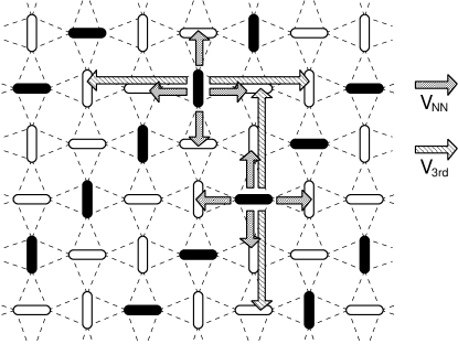
FIG. 4.: Stripe SDW structure at $m/m_{\rm sat}=1/3$, which is stabilized by the anisotropic repulsion $V_{\rm 3rd}$. Black bonds denote dimer triplet excitations and white ones dimer singlets. Arrows show range of repulsive interactions.

B Supersolid on non-plateau states

By applying a stronger magnetic field than the critical value, the plateau states continuously change to supersolid states in which superfluid components appear and coexist with SDW of the plateau states. Since the appearance of the superfluid component is accompanied by the Goldstone bosons, the plateau gap collapses.

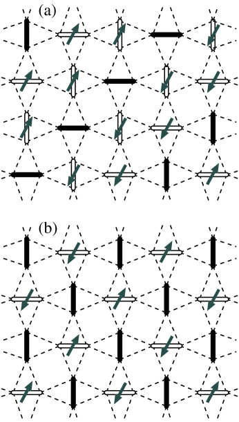
FIG. 5.: Spin configurations in supersolid phases slightly above $m/m_{\rm sat}=1/3$ (a) and 1/2 (b). Black bonds denote dimer triplet excitations and white ones with arrows denote linear combination of dimer triplet and singlet, which can be written as eq. (37). The SDW components equal to those at $m/m_{\rm sat}=1/3$ and $1/2$, respectively. Superfluid components of magnetic excitations exist on white bonds, and arrows on white bonds denote phases $\Phi$ of particles (pseudo spins). The original spin configuration is recovered by eq. (37).

Above the magnetization $m/m_{\rm sat}=1/3$, particles with density 1/3 still form SDW with the stripe structure, which equals to the one at $m/m_{\rm sat}=1/3$, and the rest of particles become superfluid in ‘canals’ between stripes. (See Fig. 5(a).) Particles can hop across a line of SDW with the help of correlated hopping terms (see Fig. 6) and this hopping makes correlations between superfluids in canals. These extra particles can Bose-condense and the phases of the superfluid particles align ferromagnetically inside an individual canal and antiferromagnetically between canals.

The supersolid state above $m/m_{\rm sat}=1/2$ maintains the same SDW as the $m/m_{\rm sat}=1/2$ case and have superfluid components as well. Phases of superfluid components form a stripe structure and the phase of one stripe aligns antiparallelly to those of next ones. (See Fig. 5(b).)

In both supersolid phases, a single dimer triplet can move by itself assisted by SDW LRO and it behaves as an elementary particle of the superfluid. The SDW forms a global network of crystallized particles and it helps a dimer triplet to hop along the network owing to the correlated hopping. We roughly evaluate the hopping of an extra particle by treating the stripe SDW as a classical background. In Fig. 6, we show the matrix element of single-dimer-triplet hopping along a stripe. Note that triplet excitations are not confined in a one-dimensional space (‘canal’) between two rows of particles. A dimer triplet can hop both parallel and perpendicular to the stripe. The superfluid component of the system may behave as an anisotropic two-dimensional Bose gas. The hopping matrices inside of a stripe are negative, whereas those across a line of triplet excitations are positive. This makes the phases of superfluid component ferromagnetic inside the stripe and antiferromagnetic between stripes.

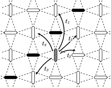
FIG. 6.: Hopping processes of a single dimer excitation (shaded one) near a line of triplet excitations (black bonds). $t_{1}=(J^{\prime})^{2}n/4J+3(J^{\prime})^{3}n/8J^{2}$, $t_{2}=-(J^{\prime})^{2}n/4J-5(J^{\prime})^{3}n/16J^{2}$, $t_{3}=-(J^{\prime})^{3}n^{2}/8J^{2}$, and $t_{4}=(J^{\prime})^{3}n^{2}/8J^{2}$. Here we assume the particle density on each black bond to be $n$. Matrices of hopping processes across the line ($t_{1}$, $t_{4}$) are all positive and other ones are negative.

A similar anisotropic superfluid was reported for the Bose-Hubbard model with frustrating interactions [34].

C Phase diagram

We show phase diagram for $J^{\prime}/J$ vs. $B/J$ at zero temperature in Fig. 7, where the phase boundaries are not very accurate. The plateau at $m/m_{\rm sat}=1/2$ appears only in the region $0<J^{\prime}/J<0.51$, and one at $m/m_{\rm sat}=1/3$ in $0<J^{\prime}/J<0.95$. For large $J^{\prime}/J$, insulating phases disappear and become superfluid phases. This is because correlated hoppings are dominant in the higher order terms and they become efficient for large $J^{\prime}/J$. The phase diagram may be not qualitatively accurate for large $J^{\prime}/J$, since our arguments are based on a strong coupling expansion. Furthermore there is a possibility that the elementary particles change to plaquette triplets[27] for large $J^{\prime}/J$, which is not taken into account in our approximation.

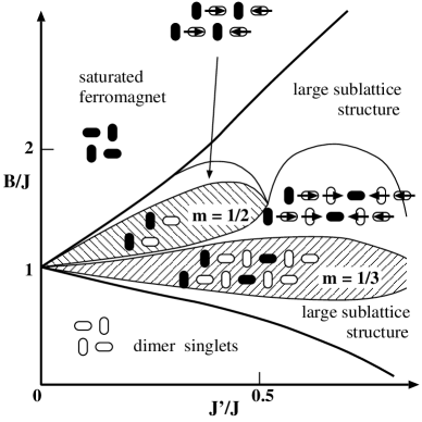
FIG. 7.: Phase diagram at $T=0$ with the parameter $J^{\prime}/J$ and the magnetic field $B/J$. The lower- and upper bold lines correspond to the 1st critical field and the saturation field, respectively. For the latter, an analytic expression is available (see section V). Inserted figures denote density-wave order and phases of particles. Black bonds denote localized particles (dimer triplets) and white ones vacancies (dimer singlets). Arrows on dimer bonds denote phases of particles.

Spin configurations at various values of magnetization are summarized as follows:

• For $0<m/m_{\rm sat}<1/3$,
  spin configuration has large sublattice structures. The system is highly frustrated and we sometimes reached to different ground states with different magnetizations in the Monte Calro method. We expect that weak interactions or quantum fluctuations can drastically change the ground state properties. One reason for this ambiguity may be that a single dimer triplet is not an elementary particle at very low magnetization, but a bound pair of triplets is. (See section IV)

• At $m/m_{\rm sat}=1/3$,
  there is only SDW LRO with stripe structure. (Fig. 4)

• For $1/3<m/m_{\rm sat}<m_{c1}$ with $0.5<J^{\prime}/J<0.8$, and for $1/3<m/m_{\rm sat}<1/2$ with $J^{\prime}/J<0.5$,
  the ground state shows supersolid with stripe structure. (Fig. 5(a))

• At $m/m_{\rm sat}=1/2$ for $J^{\prime}/J<0.5$,
  there is only SDW LRO with checkerboard structure. (Fig. 6(b) in Ref. [6].) The results of the exact diagonalization (Figs. 2(a) and (b)) indicate that this phase seems to be more stable than in our approximation because of quantum fluctuations. The phase boundary at $J^{\prime}/J=0.51$ might move to a larger value due to quantum effects. One possible reason for this discrepancy is that our classical approximation favors wave-like states (e.g. superfluid) against the localized state.

• For $1/2<m/m_{\rm sat}<m_{c2}$, if $J^{\prime}/J<0.5$,
  spins become supersolid with stripe structure. (Fig. 5(b))

• For $m_{c1}<m/m_{\rm sat}<1$ with $0.5<J^{\prime}/J$, and for $m_{c2}<m/m_{\rm sat}<1$ with $J^{\prime}/J<0.5$,
  large sublattice structures, e.g. a helical structure, appear. We will discuss nearly saturated region in Section V. A new quantum phase may appear in this region.

IV Bound state of two dimer triplets near $m=0$

In this section, we consider a striking effect of correlated hopping on the dynamics of the Shastry-Sutherland model. It is most clearly seen in the low-magnetization region where the number of magnetically excited triplets is small.

First we suppose that there are only two excited triplets. When they are far apart from each other, an individual triplet can hardly hop[17] and it gains little energy by moving on a lattice. (This almost localized property was actually observed in inelastic neutron-scattering experiments[21].) On the other hand, when the two are adjacent to each other, the situation is completely different. From the effective Hamiltonian, we can easily see that correlated-hopping processes make coherent motion of two triplets possible, where a pair of triplet dimer excitations form a bound state with $S^{z}=2$. (In the same way we can easily derive various bound states with $S=0$, 1, 2 at zero magnetic field[25]. Here we only discuss the state with $S^{z}=2$, which becomes dominant under the magnetic field.)

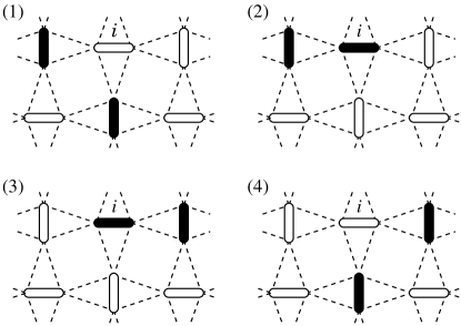
FIG. 8.: Four bases $|i,1\rangle$ (1), $|i,2\rangle$ (2), $|i,3\rangle$ (3), and $|i,4\rangle$ (4) of a bound state of two dimer triplets.

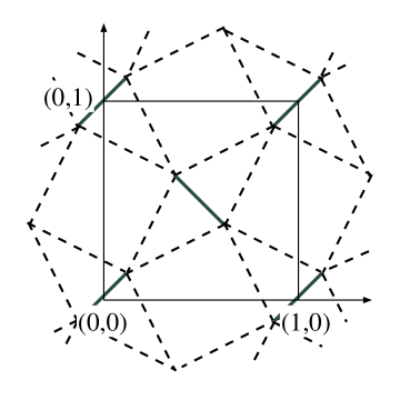
FIG. 9.: Chemical unit cell of the Shastry-Sutherland lattice.

Using the effective Hamiltonian, we can exactly show bound states. Because of the correlating hoppings, one triplet excitation exists necessarily in nearest neighbor or next nearest neighbor sites of the other. A little calculation shows that the hopping processes are decomposed into the center-of-mass motion and the relative motion, and that the latter is closed within the four states shown in Fig. 8. Hence we can write the pair excited states as

$$\sum_{i\in A}\exp(i{\bf P}\cdot{\bf r}_{i}) \{ c_{1}({\bf P})|i,1\rangle+c_{2}({\bf P})|i,2\rangle+c_{3}({\bf P})|i,3\rangle$$ (42)

$$+c_{4}({\bf P})|i,4\rangle\},$$

where the two-dimensional momenta $\mbox{\bf P}=(p_{x},p_{y})$ are defined with respect to the chemical unit cell of the Shastry-Sutherland lattice and unit vectors are defined in Fig. 9. (In this sense, the readers should not be confused our P with that used in refs. [35] and [21].) The energy spectra $\omega_{j}(\mbox{\bf P})$ ($j=1,2,3,4$) of them are computed by diagonalizing the following hopping matrix:

$$\left(\begin{array}[]{cccc}2V_{0}+V_{\rm NNN}&J_{\rm NN}&J_{\rm NN}\mbox{e}^{iP_{y}}&0\\ J_{\rm NN}&2V_{0}+V_{\rm NN}&J_{3rd}&-J_{\rm NN}\mbox{e}^{-iP_{x}}\\ J_{\rm NN}\mbox{e}^{-iP_{y}}&J_{3rd}&2V_{0}+V_{\rm NN}&-J_{\rm NN}\\ 0&-J_{\rm NN}\mbox{e}^{iP_{x}}&-J_{\rm NN}&2V_{0}+V_{\rm NNN}\end{array}\right),$$ (43)

where

$$V_{0} = J-B-\frac{\displaystyle{J^{\prime 2}}}{\displaystyle{J}}-\frac{\displaystyle{J^{\prime 3}}}{\displaystyle{2J^{2}}},$$ (44)

$$J_{\rm NN} = \frac{\displaystyle{J^{\prime 2}}}{\displaystyle{4J}}+\frac{\displaystyle{5J^{\prime 3}}}{\displaystyle{16J^{2}}},$$ (45)

$$V_{\rm NN} = \frac{\displaystyle{J^{\prime}}}{\displaystyle{2}}+\frac{\displaystyle{J^{\prime 2}}}{\displaystyle{2J}}-\frac{\displaystyle{J^{\prime 3}}}{\displaystyle{8J^{2}}},$$ (46)

$$V_{\rm NNN} = \frac{\displaystyle{J^{\prime 3}}}{\displaystyle{4J^{2}}},$$ (47)

$$J_{\rm 3rd} = \frac{\displaystyle{J^{\prime 2}}}{\displaystyle{4J}}+\frac{\displaystyle{3J^{\prime 3}}}{\displaystyle{8J^{2}}}.$$ (48)

In addition, there is another type of correlated motion obtained from the above one by reversing the space about $y$ axis. Roughly speaking, this corresponds to the interchange of dimers A and B, and its spectra are given by $\omega_{j}(-p_{x},p_{y})$. These branches together with a dispersionless band of a pair isolated triplets give the entire spectra of two-triplet sector.

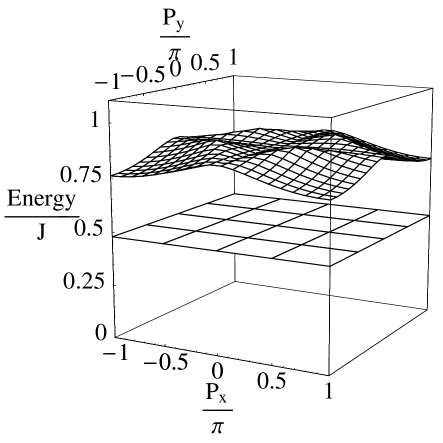
FIG. 10.: Energy spectrum of the effective Hamiltonian up to 3rd order at $J^{\prime}/J=0.63$. A two-triplet bound state consists of four branches and we show only the lowest one (see the upper band), which is apparently lower than the two-particle threshold. The spectrum of a single dimer triplet excitation ($V_{0}$) is also shown (lower band. Note that it is dispersionless at this order.)

Since these bound states can move because of correlated hopping process, energy spectra of these states are dispersive. We show only the lowest branch in Fig. 10. The lowest energy is given at $\mbox{\bf P}=(\pi,\pi)$ as

$$\Delta E_{2}(B) = 2\,V_{0}+\frac{1}{2}\left\{-J_{\rm 3rd}+V_{\rm NN}+V_{\rm NNN}\right.$$ (50)

$$\left.-\sqrt{\left(J_{\rm 3rd}-V_{\rm NN}+V_{\rm NNN}\right)^{2}+16J^{2}_{\rm NN}}\right\}.$$

On the other hand, two independent dimer triplet excitations (scattering state) have the dispersionless energy $2\Delta E_{1}(B)=2V_{0}$ (small dispersion appears at 6th order and higher [17, 35]). Expanding the right-hand side of eq.(50) in $J^{\prime}/J$, we can readily verify that there is a gain in kinetic energy of $-J(J^{\prime}/J)^{3}/4$ from the 2-particle threshold. Actually, the lowest energy of the bound state is smaller than that of two independent dimer triplets state for any $J^{\prime}/J$ as shown in Fig. 11. For example, for $J^{\prime}/J=0.68$ and $B=0$, the dispersion of a bound state takes the minimal value $0.442J$ at $\mbox{\bf P}=(\pi,\pi)$, whereas two independent dimer triplets have the energy $0.761J$ in total. As is easily seen, two triplets combined to form the $S=2$ bound states actually feel repulsive interactions between each other (i.e. $V_{\rm NN},V_{\rm NNN}>0$). Since strong repulsion $V_{\rm NN}$ acts for a pair on adjacent bonds, one may naively expect that such bound motions are not energetically favorable. However, we can take an optimal linear combination of the four relative configurations $|i,\alpha\rangle$ with $\alpha=1,2,3,4$, so that the bound state may avoid the effect of $V_{\rm NN}$ (note that only $|i,2\rangle$ and $|i,3\rangle$ feel the repulsion $V_{\rm NN}$) while gaining the kinetic energy by the coherent motion. For large $V_{\rm NN}$ we can easily verify that the effect of $V_{\rm NN}$ is canceled in $\Delta E_{2}$. The energy gain due to the motion is larger than the cost from repulsion, and hence relatively stable bound states are formed.

FIG. 11.: Energy of two dimer triplets for various $J^{\prime}/J$. Dashed line denotes the energy of two non-interacting dimer triplets ($2V_{0}$) and solid line the energy of the bound state of two dimer triplets with the momentum ($\pi,\pi$).

Next, we apply a magnetic field in the $z$-direction. Because $S^{z}=2$ bound states have lower energy than two unbound triplets, the bottom of the bound states first touches the ground state when the field is increased and one-triplet excitation still has a finite energy gap at the critical magnetic field. By increasing the magnetic field more than the critical field, a macroscopic number of bound states condense instead of the single dimer triplets. Thus the non-plateau state at very low magnetization may be a superfluid of bound states and is different from the almost localized dimer triplet state discussed by Miyahara and Ueda[17]. The critical magnetic field of magnetization process, where the magnetization starts to increase from zero, corresponds to half of the energy gap $\Delta E_{2}(0)$. If we regard the slow increase of magnetization below $H_{1}=22.5$[T][16] as the consequence of bound state condensation, we can estimate the gap $\Delta E_{2}(0)$ as $51.0$[K] from magnetization process[16, 20]. On the other hand the one-triplet energy gap $\Delta E_{1}(0)$ is estimated as $34.7$[K] from susceptibility[16], inelastic neutron scattering[21], and ESR[22]. If we set the parameters as $J=81.4$[K] and $J^{\prime}=53.5$[K], estimates of the energy gaps, $\Delta E_{1}(0)$ and $\Delta E_{2}(0)$, coincide with the experimental results.

We expect that these bound states are destroyed at higher magnetization. Indeed, one-triplet excitations can move around above $m/m_{\rm sat}=1/3$, as discussed in section III B, and they can gain more kinetic energy than bound states. There must be a transition of elementary particles from bound states for very low magnetization to one-triplet states for high magnetization. We can see this transition, if we neglect interactions between particles and apply mean-field approximation to the correlated hopping term. As particle density is increased, one-particle hopping process effectively appears as $(b_{i}^{\dagger}b_{j}+\mbox{\rm H.c.})\langle n\rangle$ from the correlated hopping term and then triplet particles gain kinetic energy. In this rough estimation, a pair of unbound triplets have lower energy than the bound state above $m/m_{\rm sat}=0.253$ for $J^{\prime}/J=0.63$. We can expect that bound states disintegrate above a finite value of magnetization and one-triplet particles turn to elementary particles. This estimate of critical magnetization can be highly modified by strong correlation and readers should not consider the above value seriously.

Finally we mention about crystallization of bound states. One may expect bound states to crystallize at low magnetization, but it will not occur. If bound states tend to crystallize, bound states loose kinetic energy and then they will be unbound by repulsive interaction between triplets.

V Near Saturation

There is another region where quantum effects manifest themselves. In this section, we briefly discuss the region just below the saturation field. In this region the one-particle excitation can be obtained from the original Shastry-Sutherland model without any approximation.

The single-particle excitation over the fully polarized ground state is given by a single flipped spin. The dispersion of this excitation is readily computed by diagonalizing the following hopping matrix

$$\left(\begin{array}[]{cccc}-\frac{1}{2}(J+4J^{\prime})&\frac{J^{\prime}}{2}(1+\mbox{e}^{-ip_{x}})&\frac{J}{2}\mbox{e}^{-ip_{x}}\mbox{e}^{-ip_{y}}&\frac{J^{\prime}}{2}(1+\mbox{e}^{-ip_{y}})\\ \frac{J^{\prime}}{2}(1+\mbox{e}^{ip_{x}})&-\frac{1}{2}(J+4J^{\prime})&\frac{J^{\prime}}{2}(1+\mbox{e}^{-ip_{y}})&\frac{J}{2}\\ \frac{J}{2}\mbox{e}^{ip_{x}}\mbox{e}^{ip_{y}}&\frac{J^{\prime}}{2}(1+\mbox{e}^{ip_{y}})&-\frac{1}{2}(J+4J^{\prime})&\frac{J^{\prime}}{2}(1+\mbox{e}^{ip_{x}})\\ \frac{J^{\prime}}{2}(1+\mbox{e}^{ip_{y}})&\frac{J}{2}&\frac{J^{\prime}}{2}(1+\mbox{e}^{-ip_{x}})&-\frac{1}{2}(J+4J^{\prime})\end{array}\right)\;.$$ (51)

In the above equation, momenta $(p_{x},p_{y})$ are defined with respect to the chemical unit cell. Reflecting the fact that a single unit cell contains four spins, the spectrum consists of four bands. Note that the four eigenvalues are invariant under the point group $\mbox{D}_{\rm 2d}$:

$$(p_{x},p_{y})\mapsto(p_{y},p_{x})\quad\mbox{and}\quad(p_{x},p_{y})\mapsto(-p_{x},p_{y})\;.$$ (52)

In the dimer limit $J^{\prime}/J\ll 1$, the lower two correspond to energy of a singlet particle on dimer bonds, where the number two comes from the two mutually orthogonal dimer bonds, and the higher two to a triplet ($S^{z}=0$) one; our approximation in section II corresponds to neglecting the latter as higher-lying.

Although the expression of the dispersion is rather complicated, we can locate the position of the band minima in the momentum space, which is relevant in determining the structure in the vicinity of saturation. For $0\leq J^{\prime}/J<1$, the lowest band takes a minimal value $-J(1+J^{\prime}/J)^{2}$ on a closed curve

$$\cos p_{x}+\cos p_{y}=2\left(\frac{J^{\prime}}{J}\right)^{2}\;.$$ (53)

This implies that magnetization saturates at

$$H_{\rm c}=J\left(1+\frac{J^{\prime}}{J}\right)^{2}\;.$$ (54)

Because of a dispersionless mode on the closed curve, the density of states (DOS) near saturation magnetization is like 1D and different from the usual 2D one. Hence the singularity of magnetization curve near saturation magnetization would be 1D-like, i.e., $|m_{\rm c}-m|\sim\sqrt{|H_{\rm c}-H|}$. This behavior can be seen in the results of the exact diagonalization in Fig. 2.

The location of the dispersion minimum $\mbox{\boldmath$p$}_{\rm min}$ together with the corresponding eigenvector determines the spin structure at the semiclassical level. Usually spin states just below the critical field are correctly given by the classical model [36, 37]. Detailed analyses of the wave functions reveal that the fourfold-degenerate classical helical order, which was pointed out by Shastry and Sutherland[18], corresponds to the four apexes $(\pm p_{\rm max},0),(0,\pm p_{\rm max})$ ($p_{\rm max}=2\cos^{-1}(J^{\prime}/J)$) of the closed curve. The fate of the classical helical LRO when the quantum effects are fully taken into account is unclear at present. The four ground states with helical LRO are connected by a gapless line, which means stiffness of helical order is vanishing. We hence expect that quantum fluctuations destroy the classical LRO.

On the other hand, for $J^{\prime}/J\geq 1$ the saturation field $H_{\rm c}=4J^{\prime}$ becomes $J$-independent and the band minimum shrinks to a single point $\mbox{\boldmath$p$}=(0,0)$; the spin structure realized in the vicinity of saturation is the classical staggered one where spins connected by $J^{\prime}$-bonds align antiferromagnetically in the $xy$-plane. Correspondingly, the transition to saturation is the same as that of 2D superfluid[40].

VI Critical Phenomena

According to an analogy to many-particle theories, a plateau state corresponds to a SDW insulating state and gapless ones to supersolids. As the plateau states at $m/m_{\rm sat}=0$, $1/3$ and $1/2$ collapse by increasing the magnetic field, superfluid components appear, whereas the SDW structure still remains in each phase. Contrary to one dimension, superfluid LRO is accompanied by the gapless Goldstone mode in our two-dimensional case. Hence, collapse of plateau occurs at the same point with the onset of superfluidity component. On the other hand if we look at the lower phase boundaries of the SDW phases, SDW structures change at the transition points in our approximation. In this case the phase transitions are presumably of first order.

Now let us consider the case of 2nd order transition. We can imagine two different situations. The first one is (i) the transitions driven by changing the external field while the coupling $J^{\prime}/J$ is kept fixed. This transition is seen in the actual magnetization process. This type of field-induced transitions has a close relationship to the filling-control insulator-to-superfluid transitions in Bose systems, and the methods used there can be imported to our case. The second one is (ii) continuous quantum phase transitions occurring with fixed values of magnetization. As the limit $J^{\prime}/J\nearrow\infty$ is approached, the Shastry-Sutherland model reduces to the ordinary $S=1/2$ square-lattice Heisenberg antiferromagnet, where no magnetization plateau appears. Hence magnetization plateaus vanish at some critical values of $J^{\prime}/J$ and are superseded by supersolid (or, superfluid) phases. In the present model, there is no particle-hole symmetry around insulating phases apparently. We hence conclude that the above two transitions have the same universality class.

First of all, we have to keep in mind that because of the special geometry of the Shastry-Sutherland model there is no a priori reason for believing that the system is described by the ordinary Bose liquid with a well-defined one-particle dispersion $\varepsilon(p)\sim p^{2}$. Actually, the low-order effective Hamiltonian (1) lacks the one-particle part. However, we have seen in section IV that this leads to the formation of dispersive two-triplet bound states in the low-field region, and in section III B that SDW structure makes one particle dispersive in the supersolid phase around $m/m_{\rm sat}=1/3$ and 1/2.

Near the phase boundaries, the superfluid amplitude is small and we can map the problem onto the effective Ginzburg-Landau model described by the superfluid order parameter [38]. (These Bose particles are not necessarily dimer triplet excitations, but they can be plaquette triplet states of two dimer triplets or flipped spin states[6].) This enables us to conclude that superfluid-onset transition would be described by the (2+1)-dimensional classical XY model when the particle-hole symmetry exists and by the $z=2$ mean-field-like transitions when it does not[39, 40]. In our case, the effective boson model in section II does not have particle-hole symmetry and we hence conclude that the plateau transition is of the dynamical exponent $z=2$ and behaves as

$$|m-m_{\rm c}| \sim |H-H_{\rm c}|\log(C/|H-H_{\rm c}|)$$ (56)

                          (2D system).

in two dimensions. Here $m_{\rm c}$ and $H_{\rm c}$ denote the critical magnetization and field at the plateau transition. In the real material, there are weak interactions between two-dimensional layers and these interactions will push the system above the upper critical dimension, i.e.

$$|m-m_{\rm c}| \sim |H-H_{\rm c}|$$ (58)

         (3D and quasi-2D systems).

Note that these forms are quite different from that in one-dimensional systems,[3] $|m-m_{\rm c}|\sim\sqrt{|H-H_{\rm c}|}$.

Here we also give a comment about the case the kinetic term of Bose particles does not behave as $\varepsilon(p)\sim p^{2}$. According to the scaling argument of Ref. [39], exponents of this kind of transitions should satisfy the relation

$$z\nu=1\;.$$ (59)

If the one-particle dispersion is of the form $\varepsilon(p)\sim p^{l}$ ($l$ denotes an even integer), the standard power-counting argument shows that the upper critical dimensions are given by $d_{\rm u}=l$. For $d\leq l$, we obtain $|m-m_{\rm c}|\sim|H-H_{\rm c}|^{d/l}$.

For the case that SDW structure changes at phase boundary, e.g. the boundary between the plateau state at $m/m_{\rm sat}=1/2$ and the supersolid one below $m/m_{\rm sat}=1/2$, the system shows a 1st order phase transition in our approximation. We don’t find any incommensurate phase between them. To take into account the possibility of any 2nd-order phase transition or incommensurate phase, we need to consider the effect of quantum fluctuations more seriously.

VII Discussions and future problems

To summarize, we studied the magnetic behavior of the Shastry-Sutherland model using strong-coupling expansion. Magnetic excitations show insulator-supersolid transitions at magnetization $m/m_{\rm sat}=1/3$ and 1/2, and thereby create magnetization plateaus. Magnetization curve obtained near $m/m_{\rm sat}=1/3$ looks similar to the experimental result.[20]

At zero magnetization, bound states of triplet excitations are formed by the correlated hopping process. Above the critical field, quintuplet ($S=2$) bound states become elementary particles in the ground state and they condense. Whereas, for large magnetization, the bound states are destroyed in the ground states and triplet excitations become elementary particles. Triplet excitations are essential for the plateau transitions at $m/m_{\rm sat}=1/3$ and 1/2. In the experiments, it is unclear in which region bound states appear as elementary particles. One possibility is that they appear in the tail of the magnetization process below $m/m_{\rm sat}\approx 0.025$. In this region, slope of the magnetization curve is different from that of rest parts.[16, 20] Further detail analysis are needed on the nature of quasiparticles.

In the present analysis, we did not find the plateaus at $m/m_{\rm sat}=1/8$ and 1/4. The mechanism of stabilizing these plateaus is not yet clear. It may be natural to believe that dimer triplet excitations are crystallized by longer-range repulsive interaction. ($S=2$ bound states cannot crystallize because of a special origin of the binding energy as we discussed in section IV.) We can consider two origins for the repulsions as follows:

• Though we cut the perturbation series at 3rd order, the higher-order expansions can produce longer-range repulsions between particles. These repulsive interactions may induce crystallization at low magnetization.

• Longer-range repulsions can come from other antiferromagnetic spin interactions in the original spin model, which have not been accounted for in the pure Shastry-Sutherland model. If we treat the antiferromagnetic interactions between next-neighbor dimer bonds, we can produce crystallization at low magnetization. For example, Müller-Hartmann et al. demonstrated the appearance of 1/4-plateau considering another spin interaction, which acts between nearest-neighbor dimers.[41]

It is unclear which spin interaction is important in the real material. We need first-principle calculation to estimate exchange couplings. We also need to keep in mind that the real material is close to the plaquette singlet phase. Under the magnetic field, if this phase becomes more stable than the dimer singlet state and plaquette triplets become elementary particles, plaquette triplets may crystallize and hence create magnetization plateaus at low magnetization as discussed in refs. [6, 27]. This should be considered in a future.

A Effective Hamiltonian

In this appendix, we briefly explain how to obtain the effective Hamiltonian in the framework of degenerate perturbation. We suppose that the ground states of the unperturbed Hamiltonian (${\cal H}_{0}$) are degenerated and we diagonalize these degenerate ground states by degenerate perturbation. Let the operators $P_{0}$ and $Q_{0}$ be the projection operators onto the degenerate (unperturbed) ground-state sector and its complement, respectively. In addition, we define a projection $P$ onto the perturbed ground-state sector.

According to ref. [42], the problem of degenerate perturbation reduces to solving the following problem

$$P_{0}{\cal H}PP_{0}|\mbox{G.S.; }\alpha\rangle=E_{\alpha}K|\mbox{G.S.; }\alpha\rangle\;,$$ (A1)

where the hermitian operator $K$ is defined by

$$K\equiv P_{0}PP_{0}\;.$$ (A2)

However, this form is not so convenient to our purpose because it does not take the form of the ordinary eigenvalue problem. A trick invented by Bloch[43] solves this difficulty. The key is to introduce a new operator $U$ through the following relation

$$PP_{0}=UK\;.$$ (A3)

The operator $U$ can be expanded as

$$U=\sum_{n=0}^{\infty}\lambda^{n}U^{(n)}\;,$$ (A4)

where the $n$-th order coefficients $U^{(n)}$ are given by

$$U^{(0)} = P_{0}$$ (A5)

$$U^{(1)} = SVP_{0}$$ (A6)

$$U^{(2)} = \left(SVSV+S^{2}VS^{0}V\right)P_{0}$$ (A7)

$$U^{(3)} = \left(SVSVSV+S^{3}VS^{0}VS^{0}V+S^{2}VSVS^{0}V\right.$$ (A10)

$$\left.+SVS^{2}VS^{0}V+S^{2}VS^{0}VSV\right)P_{0}$$

$$\cdots$$

In the above equation, we have used a short-hand notation $S^{k}$ defined by

$$S^{k}\equiv\left\{\begin{array}[]{ll}-P_{0}&\mbox{ for }k=0\\ \frac{1}{(E-{\cal H}_{0})^{k}}Q_{0}&\mbox{ for }k\geq 1\;.\end{array}\right.$$ (A11)

Then, eq. (A1) can be recasted as

$$\left(P_{0}{\cal H}U-E_{\alpha}\right)K|\mbox{G.S.; }\alpha\rangle=0\;.$$ (A12)

This is a usual eigenvalue problem and the matrix we have to diagonalize is finally given by

$${\cal H}_{\rm eff} = P_{0}{\cal H}U$$ (A13)

$$= E_{0}+\lambda P_{0}VP_{0}+\lambda^{2}P_{0}V\frac{1}{E_{0}-{\cal H}_{0}}Q_{0}VP_{0}$$ (A16)

$$\;\;+\lambda^{3}\left[P_{0}V\frac{1}{E_{0}-{\cal H}_{0}}Q_{0}V\frac{1}{E_{0}-{\cal H}_{0}}Q_{0}VP_{0}\right.$$

$$\left.-P_{0}V\frac{1}{(E_{0}-{\cal H}_{0})^{2}}Q_{0}VP_{0}VP_{0}\right]+\cdots.$$

Note that non-hermitian terms appear in general when we proceed to terms higher than second order. Reality of the eigenvalues is no longer guaranteed. To remedy this shortcomings, we have used the average of ${\cal H}_{\rm eff}$ and ${\cal H}^{\dagger}_{\rm eff}$, which is now hermitian.

REFERENCES

- [1] On leave of absence from Institute of Physics, University of Tsukuba, Tsukuba, Ibaraki 305-8571, Japan.
- [2] Y. Narumi, M. Hagiwara, R. Sato, K. Kindo, H. Nakano, and M. Takahashi, Physica B 246-247, 509 (1998); Y. Narumi, R. Sato, K. Kindo, and M. Hagiwara, J.Mag.Mag.Mat. 177-181, 685 (1998), and references cited therein.
- [3] K. Totsuka, Phys. Rev. B 57, 3454 (1998).
- [4] A. K. Kolezhuk, Phys. Rev. B, 59, 4181 (1999).
- [5] T. Momoi, H. Sakamoto, and K. Kubo, Phys. Rev. B, 59, 9491 (1999).
- [6] T. Momoi and K. Totsuka, Phys. Rev. B 61, 3231 (2000).
- [7] H. Suematsu, K. Ohmatsu, K. Sugiyama, T. Sakakibara, M. Motokawa and M. Date, Solid State Commun. 40, 241 (1981); T. Sakakibara, K. Sugiyama, M. Date and H. Suematsu, Synthetic Metals, 6, 165 (1983).
- [8] H. Nojiri, Y. Tokunaga and M. Motokawa, J. Phys. (Paris) 49 Suppl. C8, 1459 (1988).
- [9] T. Inami, Y. Ajiro, and T. Goto, J. Phys. Soc. Jpn. 65, 2374 (1996).
- [10] H. Nishimori and S. Miyashita, J. Phys. Soc. Jpn. 55, 4448 (1986).
- [11] A.V. Chubukov and D.I. Golosov, J. Phys. Cond. Matter 3, 69 (1991).
- [12] A. E. Jacobs, T. Nikuni and H. Shiba, J. Phys. Soc. Jpn. 62, 4066 (1993).
- [13] K. Kubo and T. Momoi, Z. Phys. B 103, 485 (1997).
- [14] Yu.E. Lozovik and O.I. Notych, Solid State Commun. 85, 873 (1993).
- [15] R.W. Smith and D.A. Keszler, J.Solid State Chem. 93, 430 (1991).
- [16] H. Kageyama, K. Onizuka, Y. Ueda, N.V. Mushnikov, T. Goto, K. Yoshimura, and K. Kosuge, Phys. Rev. Lett. 82, 3168 (1999); H. Kageyama, K. Onizuka, T. Yamauchi, Y. Ueda, S. Hane, H. Mitamura, T. Goto, K. Yoshimura, and K. Kosuge, J. Phys. Soc. Jpn. 68, 1821 (1999).
- [17] S. Miyahara and K. Ueda, Phys. Rev. Lett. 82, 3701 (1999).
- [18] S. Shastry and B. Sutherland, Physica 108B, 1069 (1981).
- [19] S. Miyahara and K. Ueda, unpublished.
- [20] K. Onizuka, H. Kageyama, Y. Narumi, K. Kindo, Y. Ueda, and T. Goto, J. Phys. Soc. Jpn. 69, 1016 (2000).
- [21] H. Kageyama, M. Nishi, N. Aso, K. Onizuka, T. Yosihama, K. Nukui, K. Kodama, K. Kakurai, and Y. Ueda, Phys. Rev. Lett. 84, 5876 (2000).
- [22] H. Nojiri, H. Kageyama, K. Onizuka, Y. Ueda, and M. Motokawa, J. Phys. Soc. Jpn. 68, 2906 (1999).
- [23] T. Rõõm, U. Nagel, E. Lippmaa, H. Kageyama, K. Onizuka, and Y. Ueda, cond-mat/9909284
- [24] P. Lemmens, M. Grove, M. Fischer, G. Güntherodt, V. N. Kotov, H. Kageyama, K. Onizuka, and Y. Ueda, cond-mat/0003094.
- [25] K. Totsuka, S. Miyahara, and K. Ueda, preprint.
- [26] M. Albrecht and B. Mila, Europhys. Lett. 34 145 (1996).
- [27] A. Koga and N. Kawakami, Phys. Rev. Lett. 84, 4461 (2000).
- [28] S. Miyahara and K. Ueda, Phys. Rev. B 61, 3417, (2000).
- [29] A. F. Andreev and I. M. Lifshitz, Zh. Eksp. Teor. Fiz. 56, 2057 (1969) [Sov. Phys. JETP 29, 1107 (1969)].
- [30] A.J. Leggett, Phys. Rev. Lett. 25, 1543 (1970).
- [31] K.S. Liu and M.E. Fisher, J. Low. Temp. Phys. 10, 655 (1973).
- [32] M.E. Fisher and D.R. Nelson, Phys. Rev. Lett. 32, 1350 (1974).
- [33] H. Matsuda and T. Tsuneto, Suppl. Prog. Theor. Phys. 46, 411 (1980).
-
[34]
E. Roddick and D. Stroud,
Phys. Rev. B 48, 16600 (1993);
A. van Otterlo and K.-H. Wagenblast, Phys. Rev. Lett. 72, 3598 (1994);
G.G. Batrouni, R.T. Scalettar, G.T. Zimanyi, and A.P. Kampf, ibid. 74, 2527 (1995). - [35] Z. Weihong, C.J. Hamer, and J. Oitmaa, Phys. Rev. B 60, 6608 (1999)
- [36] E.G. Batyev and L.S. Braginskii, Zh. Eksp. Teor. Fiz. 87, 1361 (1984) [Sov. Phys. JETP 60, 781 (1984)].
- [37] S. Gluzman, Phys. Rev. B 49, 11962 (1994).
- [38] S. Doniach, Phys. Rev. B 24, 5063 (1981).
- [39] M. P. A. Fisher, P. B. Weichman, G. Grinstein, and D. S. Fisher, Phys. Rev. B 40, 546 (1989).
-
[40]
D. S. Fisher and P. C. Hohenberg, Phys. Rev. B
37, 4936 (1988);
V.N. Popov, Functional Integral and Collective Excitations, Chap.6, (Cambridge University Press, 1987). - [41] E. Müller-Hartmann, R. R. P. Singh, C. Knetter, and G. S. Uhrig, Phys. Rev. Lett. 84, 1808 (2000).
- [42] T. Kato, Perturbation Theory for Linear Operators, (Springer-Verlag, Berlin, 1976).
- [43] C. Bloch, Nucl. Phys. 6, 329 (1958).