Two-dimensional dilute Bose gas in the normal phase

Abstract

We consider a two-dimensional dilute Bose gas above its superfluid transition temperature. We show that the t-matrix approximation corresponds to the leading set of diagrams in the dilute limit, provided the temperature is sufficiently larger than the superfluid transition temperature. Within this approximation, we give an explicit expression for the wave vector and frequency dependence of the self-energy, and calculate the corrections to the chemical potential and the effective mass arising from the interaction. We also argue that the breakdown of the t-matrix approximation, which occurs upon lowering the temperature, provides a simple criterion to estimate the superfluid critical temperature for the two-dimensional dilute Bose gas. The critical temperature identified by this criterion coincides with earlier results obtained by Popov and by Fisher and Hohenberg using different methods. Extension of this procedure to the three-dimensional case gives good agreement with recent Monte Carlo data.

]

I Introduction

Renewed interest in two-dimensional (2D) superfluid systems has been recently prompted by the discovery of high-temperature superconductors. Before that, studying 2D bosonic systems was mainly motivated by experiments on adsorbed helium monolayers[2] and spin-polarized hydrogen recombining on a helium film.[3] More recently, Bose condensation has been achieved experimentally in dilute gases of alkali atoms[4] and in atomic hydrogen,[5] stimulating active research in this field both experimentally and theoretically.[6]

Even though Bose-Einstein condensation is known not to occur at finite temperature for the ideal and interacting boson systems both in one and two dimensions, the absence of a condensate does not necessarily imply the lack of a phase transition to a superfluid state for an interacting 2D Bose system.[7] In this system, particles with small momenta behave like a condensate and are responsible for the presence of a nonvanishing superfluid density.[8] The critical temperature for the superfluid phase transition was estimated by Popov[8] using a functional integral formalism. The same estimate for the critical temperature was later obtained by Fisher and Hohenberg[9] using a renormalization-group approach, with the result

$$T_{c}\approx\frac{2\pi n}{m\ln{\ln{\left[1/(nr_{0}^{2})\right]}}}\;\;,$$ (1)

where $n$ is the particle density, $m$ the boson mass, and $r_{0}$ the range of the interaction potential between bosons (we set $\hbar=k_{B}=1$ throughout). In these studies, Popov[8] and Fisher and Hohenberg[9] approached the phase transition from the superfluid phase and the normal phase, respectively.

The present paper studies the 2D dilute Bose gas above its critical temperature $T_{c}$ by relying on conventional diagrammatic methods. [The criterion for a 2D Bose system to be “dilute” will be specified below.] In this way, results for thermodynamic quantities (like the critical temperature and the chemical potential) are most readily obtained. In addition, these results are amenable to extension to more complex systems, such as the composite bosons occurring in the BCS to Bose-Einstein crossover problem.[10] Finally, our method enables us to treat on equal footing the dilute Bose gas both in two and three dimensions.

Previous studies of the 2D dilute Bose gas have considered the superfluid phase either at zero temperature[11, 12, 13, 14] or at finite temperature.[8, 15] At finite temperature, the absence of a condensate in 2D required either the separation of wave-vector integration into rapid and slow parts,[8] or the use of appropriate renormalization group methods.[15] Previous approaches to the 2D dilute Bose gas, however, did not address the following issues: (i) The description of the normal phase (above the critical temperature) by standard diagrammatic methods. (ii) Upon lowering the temperature, the detection by these methods of a superfluid phase transition not associated with the establishing of long-range order.

In this respect, standard many-body diagrammatic methods prove sufficient for a complete description of the normal phase of the 2D dilute Bose gas. In particular, the t-matrix approximation for the self-energy will be shown to provide the correct description for a dilute Bose gas above $T_{c}$, akin to the three-dimensional (3D) case. Both in 2D and in 3D, an explicit analytic expression for the self-energy as a function of wave vector and frequency will be presented.

In our approach, the expression (1) for the critical temperature obtained by Popov[8] and by Fisher and Hohenberg[9] appears as a lower bound for the validity of the t-matrix as a controlled approximation for the dilute Bose gas. The ensuing diagrammatic classification scheme for the dilute Bose gas will, in fact, be shown to break down when the temperature $T$ approaches a lower temperature $T_{L}$, which coincides with the estimate (1) for the critical temperature given in Refs.[8] and[9]. In this way, the occurrence of a superfluid phase transition enters the diagrammatic theory for the dilute Bose gas, since the physical mechanism leading to a breakdown of diagrammatic perturbation theory can only be the presence of a phase transition. In addition, by applying our method to the 3D case we obtain $(T_{L}-T_{{\rm BE}})/T_{{\rm BE}}\sim n^{1/3}a$, where $T_{{\rm BE}}$ is the 3D Bose-Einstein temperature and $a$ is the scattering length, in agreement with recent Monte Carlo simulations[16, 17] on the 3D dilute Bose gas which yield for the critical temperature $T_{c}$ the same result we obtain for $T_{L}$.

The paper is organised as follows. Section 2 sets up the diagrammatic theory for the 2D dilute Bose gas in the normal phase and calculates the corrections to the chemical potential and the effective mass due to the interaction. Section 3 discusses the occurrence of the superfluid phase transition for the dilute Bose gas through a breakdown of the approximations introduced in Section 2. The value of the breakdown-temperature $T_{L}$ is then given both in two and three dimensions. Section 4 gives our conclusions. In the Appendix, the full dependence of the t-matrix self-energy on wave vector and frequency is obtained both in 2D and in 3D by exploiting the diluteness condition. In addition, the validity of some approximations on which the theoretical arguments of the text rely is explicitly tested numerically.

II t-matrix approximation for a dilute system of interacting bosons

In this Section, we analyze the diagrammatic theory for the 2D Bose gas in the normal phase and determine the leading contributions to the self-energy in the dilute limit. We give an analytic expression for the wave-vector and frequency dependence of the self-energy, which becomes asymptotically exact in the dilute limit (as verified in the Appendix). We further use the zero wave-vector and frequency value of this self-energy to dress the single-particle Green’s functions of the theory in a self-consistent way. This step will enable us to identify a lower temperature $T_{L}$ below which the classification of diagrams for the dilute Bose system breaks down, as discussed in the next Section. In addition, we obtain the explicit leading corrections to the chemical potential $\mu$ due to interaction, thus recovering an earlier result by Popov[8], and to the effective mass.

We begin by considering a 2D bosonic system interacting via a short-range two-body potential $v({\bf r})$ with a finite range $r_{0}$, which becomes a $\delta$-function when $r_{0}\to 0$ (cf. Ref. [13]). We examine the dilute limit of this system, which is initially identified by the condition $nr_{0}^{2}\ll 1$, where $n$ is the bosonic density. [A stronger condition on the parameter $nr_{0}^{2}$ will be required below.] We further consider temperatures above a nominal critical temperature $T_{c}$ but lower than an upper temperature of the order of $T_{n}\equiv 2\pi n/m$, at which quantum effects become important.[18]

Under these assumptions, the selection of the diagrams yielding the leading contributions to the self-energy for the 2D dilute Bose gas in the normal state proceeds along similar lines as for the 3D dilute Bose gas.

Akin to the 3D case, also in 2D every cycle (defined as a closed path constructed by a sequence of “bare” bosonic propagators, with a common wave vector and Matsubara frequency flow) introduces a Bose function $(e^{({\bf q}^{2}/(2m)-\mu)/T}-1)^{-1}$, which appears after the summation over the common frequency running along the cycle is performed. This function, in turn, cuts off the integral over the remaining wave-vector variable approximately at $|{\bf q}|\simeq(mT)^{1/2}$, which is much smaller than the cutoff $1/r_{0}$ introduced by the potential (owing to the the diluteness condition and the assumption $T\sim T_{n}$).

The description of the dilute Bose gas accordingly retains only those diagrams with a minimal number of cycles, that is, just one cycle. These diagrams are shown in Fig. 1(a) and constitute the so-called t-matrix approximation for the self-energy. [8, 19]

FIG. 1.: (a) t-matrix approximation for the self-energy of an interacting Bose gas; (b) Particle-hole bubble; (c) Particle-particle bubble.

At $T\sim T_{n}$ higher-order diagrams can be estimated by replacing the bare potential by the t-matrix itself and assigning to each additional cycle a factor $t_{0}\Pi_{{\rm ph}}(0)$. Here, $t_{0}$ and $\Pi_{{\rm ph}}(0)$ are the zero frequency and wave-vector values of the t-matrix and of the particle-hole bubble (Fig. 1(b)), respectively. It will further shown below that the product $t_{0}\Pi_{{\rm ph}}(0)\propto 1/\ln[1/(nr_{0}^{2})]\ll 1$ in the dilute limit.

We will verify, however, that the classification of diagrams based on the cycle argument breaks down upon lowering the temperature down to a value $T_{L}$. More precisely, we will find that the t-matrix correctly describes the dilute Bose gas in the temperature range $T_{L}\lesssim T\lesssim T_{n}$, in the sense that no other diagrams besides the t-matrix itself need to be included.

The self-energy corresponding to the set of diagrams depicted in Fig. 1(a) reads:

$$\Sigma_{t}(q)=-T\sum_{\omega_{\nu^{\prime}}}\int\!\frac{d^{2}{\bf q}^{\prime}}{(2\pi)^{2}}G(q^{\prime})\left[t\left(\frac{{\bf q}^{\prime}-{\bf q}}{2},\frac{{\bf q}^{\prime}-{\bf q}}{2},q+q^{\prime}\right)\right.$$ (2)

$$+t\left.\left(\frac{{\bf q}-{\bf q}^{\prime}}{2},\frac{{\bf q}^{\prime}-{\bf q}}{2},q+q^{\prime}\right)\right]$$ (3)

where the t-matrix $t({\bf p},{\bf p}^{\prime},P)$ is defined by the integral equation

$$t({\bf p},{\bf p}^{\prime},P) = v({\bf p}-{\bf p}^{\prime})-T\sum_{\omega_{\nu}}\int\frac{d^{2}{\bf q}}{(2\pi)^{2}}\;v({\bf p}-{\bf q})$$ (4)

$$\times G\left(\frac{P}{2}-q\right)G\left(\frac{P}{2}+q\right)t({\bf q},{\bf p}^{\prime},P)$$ (5)

with the notation $q\equiv({\bf q},i\omega_{\nu})$ ($\omega_{\nu}=2\pi\nu T$ - $\nu$ integer - being a bosonic Matsubara frequency). [20]

To lowest order in the density, all single-particle Green’s functions $G$ in Eqs. (3) and (5) are considered to be bare ones. Quite generally, self-energy insertions in the Green’s functions become relevant when the phase transition is approached. It is shown in the Appendix that, in the dilute limit, the dependence of the self-energy $\Sigma_{t}(q)$ on $q$ can be disregarded when calculating physical quantities, so that one may set $\Sigma_{t}(q)\simeq\Sigma_{t}(0)$ in all single-particle Green’s functions entering Eqs. (3) and  (5) and re-absorb the constant $\Sigma_{t}(0)$ by a shift of the chemical potential. In this way, when the chemical potential is expressed in terms of $n$ and $T$, one obtains

$$\mu-\Sigma_{t}(0)=\mu_{0}$$ (6)

where $\mu_{0}=\mu_{0}(n,T)$ is the chemical potential of the 2D ideal Bose gas.[22]

In the following, we shall consider all Green’s functions in Eqs. (3) and (5) to be self-consistently dressed by the self-energy (3) with $q=0$, resulting in an “improved” t-matrix approximation which can be adopted to approach the critical temperature more closely.

The explicit expression of $\Sigma_{t}(q)$ for arbitrary values of $q$ is given by Eq. (A12) of the Appendix, which is asymptotically valid in the dilute limit. From that expression, the shift of the chemical potential due to interaction as well as the relevant effective mass can be obtained. For the chemical potential, it is sufficient to know the value of $\Sigma_{t}(0)$, which from Eq. (A12) becomes:[21]

$$\Sigma_{t}(0)\approx\frac{8\pi n}{m\ln\left[1/(m|\mu_{0}|r_{0}^{2})\right]}$$ (7)

By entering in this expression the analytic form of the chemical potential $\mu_{0}$,[22] we obtain eventually

$$\Sigma_{t}(0) \approx \frac{8\pi n/m}{\ln(1/[mTr_{0}^{2}|\ln(1-e^{-T_{n}/T})|])}$$ (8)

$$\approx \frac{8\pi n/m}{\ln[1/(nr_{0}^{2})]+\ln[T_{n}/(2\pi T)]-\ln|\ln(1-e^{-T_{n}/T})|}$$ (9)

$$\approx \frac{8\pi n}{m\ln\left[1/(nr_{0}^{2})\right]}$$ (10)

the last result holding for $T_{n}/\ln[1/(nr_{0}^{2})]\ll T\lesssim T_{n}$, which includes the temperature range ($T_{L}\lesssim T\lesssim T_{n}$) of physical interest. Equation (10) provides the leading self-energy term for the 2D dilute Bose gas in the normal state, from which the shift of the chemical potential is obtained as $\mu=\mu_{0}+\Sigma_{t}(0)$.

Note that the expression (10) is temperature independent in the temperature range $T_{L}\lesssim T\lesssim T_{n}$ we are considering. The only temperature dependence of $\mu$ thus originates from $\mu_{0}$. In particular, at $T=T_{c}$ we substitute the value of $T_{c}$ from Eq. (1) onto the expression (10), yielding:

$$\mu(T_{c}) = \mu_{0}(T_{c})+\Sigma_{t}(0)$$ (11)

$$\approx -\frac{2\pi n}{m\ln\left[1/(nr_{0}^{2})\right]}\frac{1}{\ln\ln[1/(nr_{0}^{2})]}+\frac{8\pi n}{m\ln\left[1/(nr_{0}^{2})\right]}$$ (12)

$$\approx \frac{8\pi n}{m\ln\left[1/(nr_{0}^{2})\right]}\;\;,$$ (13)

provided that $\ln\ln(1/(nr_{0}^{2})$ is sufficiently larger than unity (dilute limit). This result coincides with the value of the chemical potential obtained in Refs. [8, 9] where the critical temperature was approached from below.

The effective mass can eventually be calculated after analytic continuation of $\Sigma_{t}(q)$. The result is

$$\frac{m^{*}}{m}=1+\frac{1}{4\ln\ln[1/(nr_{0}^{2})]}\;.$$ (14)

Details of the derivation of Eq. (14) are reported in the Appendix.

III Breakdown of the bosonic t-matrix approximation and the superfluid phase transition

We pass now to show that the selection of diagrams made in the previous Section, which was based on the cycle argument, breaks down upon lowering the temperature when the superfluid phase transition is approached. Specifically, consideration of the temperature at which the particle-hole diagrams (which where discarded by the cycle argument) are no longer negligible in comparison with the particle-particle diagrams, will lead us to identify a lower temperature $T_{L}$ that turns out to coincide with the critical temperature (1) determined in Refs.[8] and[9].

To determine the range of validity of the t-matrix approximation, it is enough to compare the particle-particle bubble $\Pi_{\rm{pp}}$ of Fig. 1(c) (which constitutes the building block of the t-matrix of Fig. 1(a)) with the particle-hole bubble $\Pi_{\rm{ph}}$ of Fig. 1(b). This statement follows from the classification of diagrams we have made because $t_{0}\simeq\Pi_{{\rm pp}}(0)^{-1}$ in the dilute limit [cf. Eqs. (A2) and (A6)], yielding $\Pi_{{\rm ph}}(0)/\Pi_{{\rm pp}}(0)$ as the small parameter of the theory at $T\sim T_{n}$. The ratio $\Pi_{{\rm ph}}(0)/\Pi_{{\rm pp}}(0)$ grows, however, upon lowering the temperature below $T_{n}$ and reaches the value of unity at the temperature $T_{L}$ introduced above.

The particle-particle bubble is given by

$$\Pi_{{\rm pp}}(0)=T\sum_{\omega_{\nu}}\int^{r_{0}^{-1}}\!\frac{d^{2}{\bf q}}{(2\pi)^{2}}\;G(q)\;G(-q)$$ (15)

where $G(q)=(i\omega_{\nu}-{\bf q}^{2}/(2m)+\mu_{0})^{-1}$ according to the arguments above. With the notation $\xi({\bf q})=|{\bf q}|^{2}/(2m)-\mu_{0}$, we obtain:

$$\Pi_{{\rm pp}}(0) = \int^{r_{0}^{-1}}\!\frac{d^{2}{\bf q}}{(2\pi)^{2}}\;\frac{1+2n_{B}(\xi({\bf q}))}{2\xi({\bf q})}$$ (16)

$$\approx \frac{m}{4\pi}\ln\left(\frac{1}{2m|\mu_{0}|r_{0}^{2}}\right)+\frac{1}{2\pi}\int_{0}^{r_{0}^{-1}}d|{\bf q}|\;\frac{|{\bf q}|\,n_{B}(\xi({\bf q}))}{\xi({\bf q})}$$ (17)

$$\approx \frac{m}{4\pi}\ln\left(\frac{1}{2m|\mu_{0}|r_{0}^{2}}\right)$$ (18)

where $n_{B}(x)=(e^{x/T}-1)^{-1}$ is the Bose function and the last asymptotic equality holds in the dilute limit $nr_{0}^{2}\ll 1$ and for temperatures of the order of $T_{n}$ (such that $|\mu_{0}|\sim T_{n}$).

The particle-hole bubble for $q=0$ is, as usual, given by $\Pi_{{\rm ph}}(0)=\partial n/\partial\mu$. For the two dimensional Bose gas the chemical potential is known analytically for all temperatures and densities[22], such that

$$\frac{\partial n}{\partial\mu}=\frac{m}{2\pi}\frac{e^{\mu_{0}/T}}{1-e^{\mu_{0}/T}}\;.$$ (19)

At $T\sim T_{n}$, $\mu_{0}(n,T_{n})\sim T_{n}$ and $\partial n/\partial\mu\sim m$, such that the ratio $\Pi_{{\rm ph}}(0)/\Pi_{{\rm pp}}(0)\approx 1/\ln[1/(nr_{0}^{2})]\ll 1$ in the dilute limit. When $T\ll T_{n}$, on the other hand, $|\mu_{0}|\ll T$ and $\partial n/\partial\mu\approx mT/(2\pi|\mu_{0}|)$, which is much larger than the corresponding value at $T\sim T_{n}$. A lower temperature $T_{L}$ can thus be reached, such that the ratio $\Pi_{{\rm ph}}(0)/\Pi_{{\rm pp}}(0)$ equals unity when

$$\frac{1}{2}\ln\frac{1}{2m|\mu_{0}|r_{0}^{2}}=\frac{T_{L}}{|\mu_{0}|}\;.$$ (20)

Entering now the asymptotic expression $|\mu_{0}|\approx Te^{-T_{n}/T}$, which holds for $T\ll T_{n}$, yields eventually

$$T_{L}\approx\frac{T_{n}}{\ln\ln[1/(nr_{0}^{2})]}$$ (21)

valid under the assumption $\ln\ln[1/(nr_{0}^{2})]\gg 1$ (which defines the diluteness condition in 2D). This expression for $T_{L}$ coincides with the estimate (1) for the critical temperature given by Popov[8] and by Fisher and Hohenberg[9]. Note that the double-log dependence of $T_{L}$ on $nr_{0}^{2}$ originates, on the one hand, from the log dependence of $\Pi_{{\rm pp}}(0)$ on $|\mu_{0}|$ and, on the other hand, from the exponential dependence of $\mu_{0}$ on $T$ at low temperatures. Note also that the more stringent diluteness condition $\ln\ln[1/(nr_{0}^{2})\gg 1$ (in the place of the original $nr_{0}^{2}\ll 1$) is required to get a finite temperature range ($T_{L}\lesssim T\lesssim T_{n}$), where self-energy diagrams can be selected by the diluteness condition.

On physical grounds, the only mechanism which may lead to the breakdown of the diagrammatic classification in terms of a small parameter (as explicitly seen above) is the occurrence of a phase transition. The breakdown temperature $T_{L}$ is thus expected to provide an estimate for the superfluid critical temperature $T_{c}$, also because the two temperatures $T_{L}$ and $T_{c}$ are expected to have the same functional dependence on $nr_{0}^{2}$, as comparison of our expression for $T_{L}$ with the value (1) for the critical temperature obtained in Refs.[8, 9] indeed shows.

Our identification of $T_{L}$ with $T_{c}$ is further confirmed by applying the same sort of arguments to the 3D dilute Bose gas, for which Monte Carlo results are available.[16, 17] In this case, the particle-particle and particle-hole bubbles are given, respectively, by

$$\Pi_{{\rm pp}}(0)\approx\frac{m}{2\pi^{2}r_{0}}=\frac{m}{4\pi a}$$ (22)

where $a$ is the scattering length, and

$$\Pi_{{\rm ph}}(0)=\frac{\partial n}{\partial\mu}\approx\frac{2mn^{1/3}}{3\zeta(3/2)^{4/3}}\frac{T_{\rm BE}}{T-T_{\rm BE}}$$ (23)

since $\mu_{0}\simeq-9\zeta(3/2)^{2}(T-T_{{\rm BE}})^{2}/(16\pi T_{\rm{BE}})$ for the chemical potential of the ideal Bose gas (valid near the Bose-Einstein temperature $T_{{\rm BE}}=2\pi/\zeta(3/2)^{2/3}n^{2/3}/m$). The temperature at which these contributions coincide then defines the 3D breakdown temperature $T_{L}^{3D}$. One obtains:

$$\frac{T_{L}^{3D}-T_{{\rm BE}}}{T_{{\rm BE}}}=\frac{8\pi}{3\zeta(3/2)^{4/3}}n^{1/3}a\simeq 2.33\,n^{1/3}a\;.$$ (24)

This result agrees with recent Monte Carlo simulations for the 3D hard-core Bose gas in the dilute limit,[17] which yielded precisely $(T_{c}-T_{{\rm BE}})/T_{{\rm BE}}=(2.3\pm 0.25)n^{1/3}a$, and coincides with the analytic result of Ref.[23], which was obtained by a completely different method.

The result (24) should be regarded as altogether non trivial, since previous analytic treatments of the 3D dilute Bose gas resulted either in different dependences of $(T_{c}-T_{{\rm BE}})/T_{{\rm BE}}$ on the parameter $n^{1/3}a$, e.g., of the type $(n^{1/3}a)^{1/2}$ [cf. Ref. [24]] or $(n^{1/3}a)^{2/3}$ [cf. Ref. [25]], or in the same linear dependence on the parameter $n^{1/3}a$, but with a different proportionality coefficient.[26, 27, 28] In our approach, the linear dependence on the parameter $n^{1/3}a$ of the temperature shift has been directly related to the quadratic dependence of the free-boson chemical potential on $T-T_{{\rm BE}}$ near $T_{{\rm BE}}$ in 3D.

IV Concluding remarks

In this paper, we have considered the two-dimensional dilute Bose gas in the normal phase, in the interesting temperature region ranging from an upper temperature $T_{n}$ (below which quantum effects become important) to a lower temperature $T_{L}$ (which we have identified as the superfluid critical temperature). In this temperature region we have analyzed the ordinary diagrammatic theory and organized it in powers of the parameter $1/\ln[1/(nr_{0}^{2})]$, which was assumed to be small compared to unity.

In this way, the standard t-matrix has been identified as yielding the dominant set of diagrams for the self-energy when $nr_{0}^{2}\ll 1$. Further analysis of the theory to define the temperature range where the t-matrix approximation holds has, however, led us to consider the stronger condition $\ln\ln[1/(na^{2})]\gg 1$ as characteristic of the “dilute” Bose gas in two dimensions, thus confirming the criterion introduced by Fisher and Hohenberg[9] via different methods.

Our identification of the lower temperature $T_{L}$ (and, thus, of the superfluid critical temperature) rests on the finding that the diagrammatic classification scheme for the 2D dilute Bose gas breaks down at this lower temperature, in the sense that additional diagrams (besides the t-matrix) become also important at $T_{L}$ and the hierarchy established for the dilute gas no longer holds. In this respect, it may be worth mentioning that our criterion to identify the critical temperature does not contradict the usual criterion which defines $T_{c}(n)$ as the temperature where the equation $\mu(n,T_{c})=\Sigma(q=0;n,T_{c})$ is satisfied. Solving, in fact, for this equation requires one to rely on an approximation for the self-energy which is valid even at $T_{c}$. We have seen, however, that in our case the t-matrix approximation for the self-energy breaks down before reaching $T_{c}$, as soon as the critical region above $T_{c}$ is approached.

The finding that an estimate of the superfluid critical temperature can be obtained from the ordinary diagrammatic theory in the normal phase, both in two and three dimensions, constitutes per se a nontrivial result, especially because the nature of the (superfluid) transition in two and three dimensions is quite different (involving, respectively, quasi-long-range order and true long-range order). In addition, our approach is rather straightforward and amenable to direct implementation to more complex physical situations.

In this respect, a possible application of our results may be the normal state of high-temperature cuprate superconductors, which are quasi-two-dimensional systems. Experiments related to the normal[29, 30] and superconducting[31] state in these systems suggest, in fact, that a correct description of their properties might require an intermediate (crossover) approach between the Fermi liquid theory (weak-coupling) and the dilute Bose gas approach (strong-coupling). For this reason, crossover theories have been considered by several authors, both for the normal state[32, 33] and the broken-symmetry phase.[34, 35] Since a reliable study of the crossover problem should require a good knowledge of at least the extreme (weak- and strong-coupling) limits, the approach developed in this paper might shed light on the strong-coupling limit of these theories.[10]

A

In this Appendix, we obtain an analytic expression for the t-matrix self-energy, which is valid above $T_{L}$ in the dilute limit. From this expression, the effective mass (at ${\bf q}=0$) is calculated. In addition, the approximation

$$\Sigma_{t}(q)\simeq\Sigma_{t}(0)$$ (A1)

(which is crucial for the arguments presented in the text) will be justified theoretically and checked numerically. Both two-dimensional and three-dimensional cases will be considered for completeness.

1 Two dimensions

It is convenient to parametrize the short-range potential by a separable potential in wave-vector space, by setting $v({\bf k}-{\bf k}^{\prime})=v_{0}w_{{\bf k}}w_{{\bf k}^{\prime}}$ with $w_{{\bf k}}=\theta(k_{0}-|{\bf k}|)$ and $k_{0}=r_{0}^{-1}$. In this way, Eq. (5) can be readily solved to yield $t({\bf p},{\bf p}^{\prime},P)=w_{{\bf p}}w_{{\bf p}^{\prime}}t(P)$, with

$$t^{-1}(P)=v_{0}^{-1}+T\sum_{\omega_{\nu}}\int\!\frac{d^{2}{\bf q}}{(2\pi)^{2}}\,w_{{\bf q}}^{2}\;G\left(\frac{P}{2}-q\right)G\left(\frac{P}{2}+q\right)\;,$$ (A2)

where $G(q)=(i\omega_{\nu}-{\bf q}^{2}/2m+\mu_{0})^{-1}$, consistently with the assumption (A1) and the ensuing Eq. (6). This choice of $G(q)$ will lead us to verify the key assumption (A1) in a self-consistent manner. The frequency sum in Eq. (A2) can be performed explicitly, yielding

$$T\sum_{\omega_{\nu}}\int\!\frac{d^{2}{\bf q}}{(2\pi)^{2}}\;w_{{\bf q}}^{2}\;G\left(\frac{P}{2}-q\right)G\left(\frac{P}{2}+q\right)$$ (A3)

$$=\int\!\frac{d^{2}{\bf q}}{(2\pi)^{2}}w_{{\bf q}}^{2}\;\frac{1+n_{B}(\xi_{{\bf P}/2-{\bf q}})+n_{B}(\xi_{{\bf P}/2+{\bf q}})}{{\bf P}^{2}/(4m)+{\bf q}^{2}/m-2\mu_{0}-i\Omega_{\nu}}\;.$$ (A4)

In the dilute limit ($nr_{0}^{2}\ll 1$) and for $T_{L}\lesssim T\lesssim T_{n}$, the Bose functions appearing in the above expression can be neglected, since they yield contributions smaller by a factor $Tr_{0}^{2}\ll 1$ with respect to the term retained. The integration over the wave vector ${\bf q}$ then yields

$$t^{-1}(P) = \frac{1}{v_{0}}$$ (A5)

$$+ \frac{m}{4\pi}\ln\left[\frac{k_{0}^{2}/m+2|\mu_{0}|+{\bf P}^{2}/(4m)-i\Omega_{\nu}}{2|\mu_{0}|+{\bf P}^{2}/(4m)-i\Omega_{\nu}}\right]$$ (A6)

where ln stands for the principal branch of the complex logarithm. The t-matrix self-energy is obtained by inserting expression (A6) into Eq. (3) which, for a separable potential, becomes

$$\Sigma_{t}({\bf q},\omega_{\nu}) = -2\;T\sum_{\Omega_{\nu^{\prime}}}\int\!\frac{d^{2}{\bf q^{\prime}}}{(2\pi)^{2}}\;w^{2}_{({\bf q}^{\prime}-{\bf q})/2}$$ (A7)

$$\times G({\bf q}^{\prime},\Omega_{\nu^{\prime}}-\omega_{\nu})t({\bf q}+{\bf q}^{\prime},\Omega_{\nu^{\prime}})\;.$$ (A8)

To perform the frequency sum in Eq. (A8) we exploit the analytic properties of $t({\bf P},z)$. From Eq. (A6), after the replacement $i\Omega_{\nu^{\prime}}\to z$, it can be readily verified that $t({\bf P},z)$ has a simple pole for $z={\bf P}^{2}/(4m)+2|\mu_{0}|+k_{0}^{2}/[m(1-e^{-1/{\tilde{v}_{0}}})]$ (with ${\tilde{v}_{0}}=mv_{0}/(4\pi)$) and a branch cut along the real axis for ${\bf P}^{2}/(4m)+2|\mu_{0}|<{\rm Re}(z)<{\bf P}^{2}/(4m)+2|\mu_{0}|+k_{0}^{2}/m$. The frequency sum in Eq. (A8) can be then performed by a contour integration, yielding three distinct contributions: one from the simple pole of the Green’s function $G({\bf q}^{\prime},z)$, one from the simple pole of the t-matrix, and one from the integration along the cut of $t({\bf q}+{\bf q}^{\prime},z)$. The term originating from the simple pole of the t-matrix, which occurs for ${\rm Re}(z)>k_{0}^{2}/m$, is exponentially suppressed by the Bose factor $1/(\exp(\beta z)-1)$ and is thus negligible. The term associated with the integration along the cut can be estimated to be smaller than the term from the simple pole of the Green’s function by a factor $1/\ln[1/(nr_{0}^{2})]$, and is also negligible in the dilute limit. We are thus left with the expression:

$$\Sigma_{t}({\bf q},\omega_{\nu})=2\int\!\frac{d^{2}{\bf{\bf p}}}{(2\pi)^{2}}\frac{w^{2}_{{\bf q}/2}}{e^{\beta[\frac{({\bf q}-{\bf p})^{2}}{2m}+|\mu_{0}|]}-1}\left[\frac{1}{v_{0}}+\frac{m}{4\pi}\phantom{\frac{k_{0}^{2}/m}{{\bf q}^{2}/m}}\right.$$ (A9)

$$\times \left.\ln\frac{k_{0}^{2}/m+|\mu_{0}|+{\bf q}^{2}/(2m)-{\bf p}^{2}/(4m)-i\omega_{\nu}}{|\mu_{0}|+{\bf q}^{2}/(2m)-{\bf p}^{2}/(4m)-i\omega_{\nu}}\right]^{-1}.$$ (A10)

Note that the Bose factor in Eq. (A10) is peaked about ${\bf p}={\bf q}$ with a width of order $T^{1/2}$, which is smaller than the range of ${\bf p}$ over which the log-term in the denominator of Eq. (A10) varies appreciably. When performing the integration over ${\bf p}$ in Eq. (A10), we can then approximate ${\bf p}={\bf q}$ in the logarithm, which is in this way factored out of the integral, yielding the following asymptotic expression for the self-energy:

$$\frac{\Sigma_{t}(q)}{2n} \approx w^{2}_{{\bf q}/2}\left\{\frac{1}{v_{0}}\phantom{\frac{k_{0}^{2}/m}{q^{2}}}\right.$$ (A11)

$$+ \left.\frac{m}{4\pi}\ln\left[\frac{k_{0}^{2}/m+|\mu_{0}|+{\bf q}^{2}/(4m)-i\omega_{\nu}}{|\mu_{0}|+{\bf q}^{2}/(4m)-i\omega_{\nu}}\right]\right\}^{-1}.$$ (A12)

The analytic expression (A12) can be compared with the numerical calculation for the t-matrix self-energy, obtained by retaining all contributions to Eq. (A8).

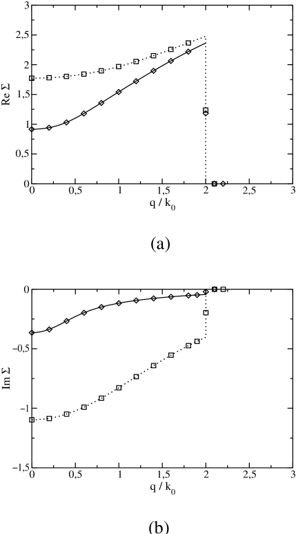
FIG. 2.: $\Sigma(q,\omega_{\nu})$ (units of $T_{n}$) for a 2D dilute Bose gas at $T=T_{n}$ and $nr_{0}^{2}=1.6\times 10^{-3}$. Numerical results for $\nu=10$ (diamonds) and $\nu=100$ (squares) are compared with the analytic expression (A12) (full and dotted lines, respectively).

We have found that the asymptotic expression (A12) reproduces extremely well the numerical results for (A8) when the diluteness parameter is sufficiently small. As an example, in Fig. 2 the analytic expression for $\Sigma_{t}(q)$ is compared with the numerical results for the choice of parameters $T=T_{n}$, $mv_{0}/(4\pi)=1$, and $nr_{0}^{2}=1.6\times 10^{-3}$. One can see that in this case the agreement is excellent.

The expression (A12) for the self-energy can also be used to verify that, when evaluating physical quantities (such as the density $n$), the wave-vector and frequency dependence of $\Sigma_{t}(q)$ is actually irrelevant, so that one can approximate $\Sigma_{t}(q)\simeq\Sigma_{t}(0)$ as anticipated in Eq. (A1). This is because the presence of the logarithm in Eq. (A12) makes the dependence of $\Sigma_{t}(q)$ on $q$ rather slow. The approximation $\Sigma_{t}(q)\simeq\Sigma_{t}(0)$ is thus justified over a large portion of $q$ space and can be exploited to evaluate physical quantities. In particular, for $T=T_{n}$ we have obtained numerically that the relative error when evaluating $n=-T\sum_{\nu}\int\frac{d^{2}{\bf q}}{(2\pi)^{2}}\;G(q)$ alternatively with $G(q)=[i\Omega_{\nu}-{\bf q}^{2}/(2m)+\mu-\Sigma_{t}(q)]^{-1}$ or with $G(q)\to G_{0}(q)=[i\Omega_{\nu}-{\bf q}^{2}/(2m)+\mu-\Sigma_{t}(0)]^{-1}$ is less than 1% for $nr_{0}^{2}\lesssim 10^{-2}$.

Finally, the t-matrix self-energy (A12) can be exploited to calculate the effective mass for the dilute Bose gas. Recall that, once the retarded self-energy is known, the effective mass can be calculated as[36]

$$\frac{m^{*}}{m}=\left(1-\frac{\partial{\rm Re}\Sigma(|{\bf q}|,\omega)}{\partial\omega}\right)\left[1+\frac{m}{|{\bf q}|}\frac{\partial{\rm Re}\Sigma(|{\bf q}|,\omega)}{\partial|{\bf q}|}\right]^{-1},$$ (A13)

where the derivatives are meant to be calculated at the quasi-particle pole defined by the equation

$$\omega_{{\bf q}}=\frac{{\bf q}^{2}}{2m}-\mu+{\rm Re}\Sigma({\bf q},\omega_{{\bf q}})\;.$$ (A14)

In general, the effective mass $m^{*}$ depends on ${\bf q}$. Here we are interested in its value at ${\bf q}=0$, which is relevant at low temperatures.

The self-energy (A12) can be analytically continued via the replacement $i\omega_{n}\to\omega+i0^{+}$. The quasi-particle-pole equation (A14) at ${\bf q}=0$ can then be solved asymptotically, to yield

$$\omega_{0}=-\mu+\Sigma_{t}(0)\left(1-2\frac{\ln\ln[1/(nr_{0}^{2})]}{\ln(1/(nr_{0}^{2})]}\right)$$ (A15)

as it can be verified by inserting the value (A15) for $\omega_{0}$ in the quasi-particle-pole equation and by discarding subleading terms in the dilute limit $nr_{0}^{2}\ll 1$. The derivatives of $\Sigma({\bf q},\omega)$ at $({\bf q}=0,\omega=\omega_{0})$ can also be readily calculated. The effective mass at ${\bf q}=0$ is then given by

$$\frac{m^{*}}{m}\approx\frac{1+1/(2\ln\ln[1/(nr_{0}^{2})])}{1-1/(4\ln\ln[1/(nr_{0}^{2})])}\approx 1+1/(4\ln\ln[1/(nr_{0}^{2})]).$$ (A16)

Note the occurrence of the same double-log dependence characteristic of the temperature $T_{L}$.

2 Three dimensions

The three-dimensional case can be treated in a parallel fashion to the two-dimensional case. By considering the same separable potential adopted in 2D, and by following the same steps which lead to Eq. (A6), we now obtain:

$$t^{-1}(P) = \frac{1}{v_{0}}+\frac{m}{2\pi^{2}}\left[k_{0}-m^{1/2}\sqrt{-2\mu_{0}+\frac{{\bf P}^{2}}{4m}-i\Omega_{\nu}}\right.$$ (A17)

$$\times \left.\arctan\frac{k_{0}/m^{1/2}}{\sqrt{-2\mu_{0}+\frac{{\bf P}^{2}}{4m}-i\Omega_{\nu}}}\right]$$ (A18)

where the complex arctan is defined, as usual, in terms of the principal branch of the complex logaritm as follows:

$$\arctan z=\frac{i}{2}\ln\frac{1-iz}{1+iz}\;.$$ (A19)

Like in 2D, the t-matrix $t({\bf P},z)$ has a branch cut along the real axis for ${\bf P}^{2}/(4m)+2|\mu_{0}|<{\rm Re}(z)<{\bf P}^{2}/(4m)+2|\mu_{0}|+k_{0}^{2}/m$, and a simple pole located along the real axis for ${\rm Re}z>{\bf P}^{2}/(4m)+2|\mu_{0}|+k_{0}^{2}/m$. Upon trasforming the frequency sum in (A8) into a contour integration, the t-matrix simple pole contribution will be again strongly suppressed by the Bose factor, while the term associated with the integration along the cut can now be proven to be smaller than the term originating from the simple pole of the Green’s function by a factor $(nr_{0}^{3})^{1/2}$. In the dilute limit, only the simple pole of the Green’s function therefore contributes to the contour integration. By the same argument leading to Eq. (A12), we obtain the following asymptotic expression for the t-matrix self-energy:

$$\frac{\Sigma_{t}(q)}{2n} \approx w^{2}_{{\bf q}/2}\left[\frac{1}{v_{0}}+\frac{m}{2\pi^{2}}\left(k_{0}-\sqrt{|\mu_{0}|+\frac{{\bf q}^{2}}{4m}-i\omega_{\nu}}\right.\right.$$ (A20)

$$\times \left.\left.m^{1/2}\arctan\frac{k_{0}/m^{1/2}}{\sqrt{|\mu_{0}|+\frac{{\bf q}^{2}}{4m}-i\omega_{\nu}}}\right)\right]^{-1}\;.$$ (A21)

The asymptotic expression (A21) has also been checked against numerical calculation of Eq. (A8) in three dimensions. In Fig. 3 the analytic expression (A21) is compared with the numerical results for the choice of parameters $T=T_{n}$, $(2\pi^{2})/(mv_{0}k_{0})\to 0$, and $n^{1/3}r_{0}=1\times 10^{-2}$. Even in 3D the agreement is excellent.

The approximation $\Sigma_{t}(q)\simeq\Sigma(0)$ has further been checked by evaluating the particle density. In this case, we have found that the error introduced by the approximation (A1) in the estimate for the density is less than 1% when $nr_{0}^{3}\lesssim 5\times 10^{-3}$.

Finally, the solution of the quasi-particle-pole equation (A14) at ${\bf q}=0$ in 3D is given by

$$\omega_{0}=-\mu+\Sigma_{t}(0)=|\mu_{0}|\;,$$ (A22)

while the retarded self-energy near the quasi-particle pole is given by

$$\Sigma({\bf q},\omega)=\frac{2n}{\frac{m}{4\pi a}-i\frac{m}{2\pi^{2}}A({\bf q},\omega)\left[\frac{\pi}{2}+\frac{i}{2}\ln\frac{\pi/(2aA({\bf q},\omega))+1}{\pi/(2aA({\bf q},\omega))-1}\right]}$$ (A23)

with $A({\bf q},\omega)=\sqrt{\omega-{\bf q}^{2}/(4m)-|\mu_{0}|}$ and where we have introduced the scattering length $a$ via the relation $m/(4\pi a)\approx(mk_{0})/(2\pi^{2})$. By using the definition (A13), the effective mass at ${\bf q}=0$ can be readily calculated, leading to the result:

$$\frac{m^{*}}{m} \approx \left[1+\frac{8\pi na^{3}}{m}\left(1+\frac{4}{\pi^{2}}\right)\right]\left[1+\frac{4\pi na^{3}}{m}\left(1+\frac{4}{\pi^{2}}\right)\right]^{-1}$$ (A24)

$$\approx 1+\frac{4\pi na^{3}}{m}\left(1+\frac{4}{\pi^{2}}\right)\;\;.$$ (A25)

Note that the interaction increases the (quasi)-particle mass both in 3D and in 2D with respect to its bare value.

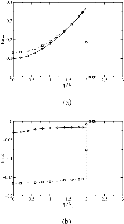
FIG. 3.: $\Sigma(q,\omega_{\nu})$ (units of $T_{n}$) for a 3D dilute Bose gas at $T=T_{n}$ and $n^{1/3}r_{0}=1\times 10^{-2}$. Numerical results for $\nu=10$ (diamonds) and $\nu=100$ (squares) are compared with the analytic expression (A21) (full and dotted lines, respectively).

REFERENCES

- [1] Permanent address: Dept. of Theoretical Physics, “Babes-Bolyai” University, 3400 Cluj, Romania.
- [2] W.D. McCornick, D.L. Goodstein, and J.G. Dash, Phys. Rev. 168, 249 (1968); G.A. Stewart and J.G. Dash, Phys. Rev. A 2, 918 (1970); J.G. Dash, Phys. Rep. 38 C, 177 (1978); D.J. Bishop and J.D. Reppy, Phys. Rev. B 22, 5171 (1980).
- [3] L.J. Lantto and R.M. Nieminen, J. Low Temp. Phys. 37, 1 (1979).
- [4] M.H. Anderson et al., Science 269, 198 (1995); C.C. Brabley et al., Phys. Rev. Lett. 75, 1687 (1995); K.B. Davis et al., Phys. Rev. Lett. 75, 3969 (1995).
- [5] D.G. Fried et al., Phys. Rev. Lett. 81, 3811 (1998).
- [6] For a review, see F. Dalfovo, S. Giorgini, L.P. Pitaevskii, and S. Stringari, Rev. Mod. Phys. 71, 463 (1999).
- [7] J.M. Kosterlitz and D.J. Thouless, J. Phys. C 6, 1181 (1973).
- [8] V.N. Popov, Functional Integrals in Quantum Field Theory and Statistical Physics (Riedel, Dordrecht, 1983); Functional Integrals and Collective Excitations (Cambridge University Press, Cambridge, 1987).
- [9] D.S. Fisher and P.C. Hohenberg, Phys. Rev. B 37, 4936 (1988).
- [10] P. Pieri, G.C. Strinati, and I. Tifrea (in preparation).
- [11] M. Schick, Phys. Rev. A 3, 1067 (1971).
- [12] D.F. Hines, N.E. Frankel, and D.J. Mitchell, Phys. Lett. 68 A, 12 (1978).
- [13] E.B. Kolomeisky and J.P. Straley, Phys. Rev. B 46, 11749 (1992).
- [14] E.H. Lieb and J. Yngvason, math-ph/0002014, J. Stat. Phys. (in press).
- [15] C. Chang and R. Friedberg, Phys. Rev. B 51, 1117 (1995).
- [16] P. Grüter, D. Ceperley, and F. Laloë, Phys. Rev. Lett. 79, 3549 (1997).
- [17] M. Holzmann and W. Krauth, Phys. Rev. Lett. 83, 2687 (1999).
- [18] R.M. May, Phys. Rev. 115, 254 (1959).
- [19] S.T. Beliaev, JETP 34, 417 (1958) [Sov. Phys. JETP 7, 289 (1958)].
- [20] The interaction vertices represented by points in the diagrams of Fig. 1 are meant to be symmetrized: . By expressing the self-energy diagrams of Fig. 1(a) in terms of unsymmetrized interaction vertices and taking into account the symmetry factor of these diagrams, Eqs. (3) and (5) follow.
- [21] Throughout this paper, we adopted the same notation of Ref. [9], with the symbol meaning “asymptotically equal”.
- [22] In two dimensions, the chemical potential of the ideal Bose gas can be evaluated analytically for all temperatures and densities, yielding [cf. Ref. [18]].
- [23] G. Baym, J.-P. Blaizot, and J. Zinn-Justin, Europhys. Lett. 49, 150 (2000).
- [24] K. Huang, Phys. Rev. Lett. 83, 3770 (1999).
- [25] H.T.C. Stoof, Phys. Rev. Lett. 66, 3148 (1991).
- [26] T.D. Lee and C.N. Yang, Phys. Rev. 112, 1419 (1958).
- [27] H.T.C. Stoof, Phys. Rev. A 45, 8398 (1992).
- [28] G. Baym, J.-P. Blaizot, M. Holzmann, F. Lalöe, and D. Vautherin, Phys. Rev. Lett. 83, 3770 (1999).
- [29] H. Ding et al., Nature 382, 51 (1996); Phys. Rev. Lett. 78, 2628 (1997).
- [30] A. G. Loeser et al. , Science 273, 325 (1996).
- [31] Y.J. Uemura et al., Phys. Rev. Lett. 62, 2317 (1989).
- [32] R. Haussmann, Z. Phys. B 91, 291 (1993).
- [33] P. Pieri and G.C. Strinati, Phys. Rev. B. 61, 15370 (2000).
- [34] M. Randeria, Ji-Min Duan, and Lih-Yir Shieh, Phys. Rev. Lett. 62, 981 (1989); Phys. Rev. B 41, 327 (1990).
- [35] F. Pistolesi and G. C. Strinati, Phys. Rev. B 53, 15168 (1996).
- [36] J.W. Negele and H. Orland, Quantum Many-Particle Systems (Addison-Wesley, New York, 1988), section 5.3.