Effects of Boson Dispersion in Fermion-Boson Coupled Systems

Abstract

We study the nonlinear feedback in a fermion-boson system using an extension of dynamical mean-field theory and the quantum Monte Carlo method. In the perturbative regimes (weak-coupling and atomic limits) the effective interaction among fermions increases as the width of the boson dispersion increases. In the strong coupling regime away from the anti-adiabatic limit, the effective interaction decreases as we increase the width of the boson dispersion. This behavior is closely related with complete softening of the boson field. We elucidate the parameters that control this nonperturbative region where fluctuations of the dispersive bosons enhance the delocalization of fermions.

]

I Introduction

Interacting fermion-boson systems are very important in condensed matter physics and have been studied intensively. [1] They are directly relevant to the description of electron-lattice interaction. Other problems can be mapped onto interacting fermions and bosons by means of the Hubbard-Stratonovich transformation. [2, 3] While the problem of a single fermion interacting with a boson field, i.e., the polaron problem, is well understood, [1] a lot less is known about the many-fermion problem in interaction with a boson field; it is a full interacting many-body problem which is only tractable analytically in the adiabatic [4] and the atomic limits. [5, 6, 1]

In this paper we revisit the interacting and dispersive fermion-boson problem using dynamical mean-field (DMT) theory. [7] This method reduces the quantum many-body problem to a quantum impurity model obeying a self-consistency condition. This method has been useful in describing strong coupling problems such as the Mott transition. There are several motivations for our work.

First, a DMF treatment of the bosonic and fermionic degrees of freedom taking into account the boson dispersion, requires an extension of the DMF equations where the bosonic propagator degrees of freedom are determined self-consistently. This represents a new type of self-consistent DMF equation, which so far has not been investigated. These equations are relevant to many problems, electron-phonon interactions, fermions interacting with spin fluctuations [8] or among themselves via the long-ranged Coulomb interactions, [9] and to the boson-fermion model. [10]

Second, while the Mott transition in the Hubbard model is well understood using DMF methods, it is interesting to understand how it is modified by the variation of the frequency of the mode that mediates the interaction, or how the results are changed by the electron-phonon interactions. The approach discussed in this paper is a first step in this direction.

Finally, phonon dispersion effects are relevant to many systems. The Jahn-Teller or breathing-type phonons, for instance, seen in manganese oxides should be dispersive due to intersite coupling. A distortion of a MnO₆-octahedron affects distortions of the neighbor octahedra, since the MnO₆-octahedra share their oxygen atoms which leads to an intersite coupling. This may be relevant to fascinating orderings of lattice and charge in doped manganites. [11, 12, 13, 14]

We study the mutual feedback of fermionic and bosonic degrees of freedom in a very simple system of fermions interacting with one branch of bosons at half filling. However the methodology can be extended to other problems where similar DMF equations occur such as electron problems with long-ranged Coulomb interactions and the competition of magnetic order and the heavy fermion state, and to the boson-fermion mixture of high temperature superconductivity.

This paper is organized as follows. In the next section we discuss how DMF theory needs to be extended to fully include the feedback effects through fermion-boson interaction. Quantum Monte Carlo (QMC) method is introduced to solve the DMF equations for all parameter regions. We also discuss some technical points of the QMC relevant to this problem. The formalism is applied to demonstrate effects of boson dispersion in a wide region of parameters and the results are summarized in Sec. III. In Sec. IV, we discuss our main result: The existence of two distinct regimes of the DMF solutions. In the first regime, the feedback effects increase the fermion-boson coupling. In the second regime, which is strongly fluctuating, the boson dispersion accelerates the delocalization of fermions. Complete softening characterizes the crossover between these regimes. Section V is devoted to summary.

II Dynamical Mean-Field Formalism and Hamiltonian

In this work, we discuss such feedback effects caused by the fermion-boson interaction using DMF theory. DMF theory provides a local view of a many-body problem in terms of an impurity model which satisfies a self-consistency condition. [7] For general fermion-boson problems with a local interaction, the local action has the form

$$S_{\rm eff} = \int d\tau d\tau^{\prime}\sum_{\alpha}c_{\alpha}^{\dagger}(\tau){\cal G}_{0\alpha}^{-1}(\tau-\tau^{\prime})c_{\alpha}(\tau^{\prime})$$ (1)

$$+ \int d\tau d\tau^{\prime}\sum_{\nu}x_{\nu}(\tau){\cal D}_{0\nu}^{-1}(\tau-\tau^{\prime})x_{\nu}(\tau^{\prime})$$ (2)

$$+ \int d\tau\sum_{\alpha_{1}\alpha_{2}\nu}\lambda_{\alpha_{1}\alpha_{2}\nu}c_{\alpha_{1}}^{\dagger}(\tau)c_{\alpha_{2}}(\tau)x_{\nu}(\tau),$$ (3)

where ${\cal G}_{0}$ and ${\cal D}_{0}$ are the bare impurity Green’s functions for fermion and boson, respectively, which contain the dynamical information of the integrated other sites. Here $c_{\alpha}$ is the fermion annihilation operator and $x_{\nu}$ is the boson field. $\lambda_{\alpha_{1}\alpha_{2}\nu}$ denotes the coupling between fermions and bosons. The index $\alpha$ ($\nu$) denotes internal degrees of freedom of fermions (bosons) such as spins or orbitals of electrons (normal modes of phonons). We do not explicitly write the contribution from fermion interactions such as the Coulomb interaction since we focus on the effects of boson dispersions in this paper. However the action (3) is quite general which contains such fermion interactions through the Hubbard-Stratonovich transformation [2, 3] with continuous fields. Of course, alternatively, one can include additionally the fermion interactions according to the DMF theory for the Hubbard-type models. [7]

The full Green’s functions are related to the bare ones by

$${\cal G}_{\alpha}^{-1}(i\omega_{n}) = {\cal G}_{0\alpha}^{-1}(i\omega_{n})-\Sigma_{\alpha}(i\omega_{n}),$$ (4)

$${\cal D}_{\nu}^{-1}(i\omega_{n}) = {\cal D}_{0\nu}^{-1}(i\omega_{n})-\Pi_{\nu}(i\omega_{n}),$$ (5)

at each Matsubara frequency $\omega_{n}=(2n+1)\pi/\beta$ for fermion and $\omega_{n}=2n\pi/\beta$ for boson, respectively ($n$ is an integer). $\beta$ is the inverse temperature. $\Sigma$ and $\Pi$ are the self-energy for fermion and boson, respectively. The Green’s functions for both fermion and boson are determined in a self-consistent way. This is achieved by the following set of self-consistency conditions,

$${\cal G_{\alpha}} = \sum_{\mbox{\boldmath$q$}}\left[i\omega_{n}+\mu-\epsilon_{\mbox{\boldmath$q$}\alpha}-\Sigma_{\alpha}(i\omega_{n})\right]^{-1},$$ (6)

$${\cal D_{\nu}} = \sum_{\mbox{\boldmath$q$}}\left[(i\omega_{n})^{2}-\omega_{\mbox{\boldmath$q$}\nu}^{2}-\Pi_{\nu}(i\omega_{n})\right]^{-1},$$ (7)

where $\epsilon_{\mbox{\boldmath$q$}\alpha}$ and $\omega_{\mbox{\boldmath$q$}\nu}$ give the dispersion relations for fermions and bosons as a function of the wave number $q$, respectively. $\mu$ is the chemical potential to control the density of fermions. Here the bosons are described as harmonic oscillators. The condition (7) is modified according to the property of boson degrees of freedom.

Previous studies of other models have indicated that the results of the DMF theory can give useful insights into three-dimensional systems. [7] We have therefore taken the dispersions $\epsilon_{\mbox{\boldmath$q$}}$ and $\omega_{\mbox{\boldmath$q$}}$ that correspond to a semicircular density of states, see the details in Sec. III A. These DMF equations are exact for a model where the fermions and the bosons have random hopping on lattice sites.

The self-consistency loop is closed as follows: The effective action (3) is solved for given bare impurity Green’s functions ${\cal G}_{0}$ and ${\cal D}_{0}$ to obtain the full Green’s functions ${\cal G}$ and ${\cal D}$. The self-energy $\Sigma$ and $\Pi$ are calculated by the relations (4) and (5), and used to obtain the Green’s functions through the self-consistency conditions (6) and (7). New bare impurity Green’s functions are calculated by the relations (4) and (5) again. This loop is iterated until all the quantities are converged. In this way, both fermionic and bosonic dispersions are renormalized through the fermion-boson interaction, and the mutual feedback effects are fully included.

The above DMF equations assume that no symmetry breaking is present in the system although the extension to phases with broken symmetry is straightforward. And they can be derived from an electron-phonon model:

$${\cal H}={\cal H}_{\rm F}+{\cal H}_{\rm B}+{\cal H}_{\rm I},$$ (8)

where

$${\cal H}_{\rm F} = \sum_{\alpha}\sum_{\mbox{\boldmath$q$}}\left(\epsilon_{\mbox{\boldmath$q$}\alpha}-\mu\right)c_{\mbox{\boldmath$q$}\alpha}^{\dagger}c_{\mbox{\boldmath$q$}\alpha}+{\cal H}_{\rm int},$$ (9)

$${\cal H}_{\rm B} = \sum_{\nu}\sum_{\mbox{\boldmath$q$}}\omega_{\mbox{\boldmath$q$}\nu}\left(a_{\mbox{\boldmath$q$}\nu}^{\dagger}a_{\mbox{\boldmath$q$}\nu}+\frac{1}{2}\right),$$ (10)

$${\cal H}_{\rm I} = \sum_{\alpha_{1}\alpha_{2}\nu}\sum_{\mbox{\boldmath$p$},\mbox{\boldmath$q$}}\tilde{\lambda}_{\mbox{\boldmath$q$}\alpha_{1}\alpha_{2}\nu}c_{\mbox{\boldmath$p$}+{\mbox{\boldmath$q$}\alpha_{1}}}^{\dagger}c_{\mbox{\boldmath$p$}\alpha_{2}}\left(a_{\mbox{\boldmath$q$}\nu}+a_{-\mbox{\boldmath$q$}\nu}^{\dagger}\right),$$ (11)

where $a_{\mbox{\boldmath$q$}}$ is the boson annihilation operator which is related with the boson field by $x_{\mbox{\boldmath$q$}}=(2M\omega_{\mbox{\boldmath$q$}})^{-1/2}(a_{\mbox{\boldmath$q$}}+a_{-\mbox{\boldmath$q$}}^{\dagger}).$

The model (8) has been intensively studied using DMF methods in the limit of zero boson dispersion, i.e., in the Holstein model: [5, 6] Bosons with the same index $\nu$ have a same frequency (Einstein phonons) and the fermion-boson coupling is local as

$${\cal H}_{\rm B} = \sum_{\nu}\omega_{0\nu}\sum_{\mbox{\boldmath$q$}}\left(a_{\mbox{\boldmath$q$}\nu}^{\dagger}a_{\mbox{\boldmath$q$}\nu}+\frac{1}{2}\right)$$ (12)

$$= \sum_{\nu}\frac{M_{\nu}}{2}\sum_{i}\left(\dot{x}_{i\nu}^{2}+\omega_{0\nu}^{2}x_{i\nu}^{2}\right),$$ (13)

$${\cal H}_{\rm I} = \sum_{\alpha_{1}\alpha_{2}\nu}\sum_{i}\lambda_{\alpha_{1}\alpha_{2}\nu}c_{i\alpha_{1}}^{\dagger}c_{i\alpha_{2}}x_{i\nu},$$ (14)

where the index $i$ denotes a lattice site. In the ground state, the possibility of charge-ordered or superconducting states has been intensively discussed for this model. [15, 16, 17, 18, 19] Above the critical temperatures of these states, the crossover behavior is observed from the Fermi liquid with a mass enhancement in the weak coupling region to the so-called polaron which is a combined object between fermion and boson in the strong coupling region. [1, 5, 6, 20]

It is instructive to compare the present framework with the DMF theory for the problem without the boson dispersions such as the Holstein model. If bosons have no dispersion, that is, all $\omega_{\mbox{\boldmath$q$}}$ take the same value $\omega_{0}$ independent of $q$, Eq. (7) is rewritten as

$${\cal D}=\left[(i\omega_{n})^{2}-\omega_{0}^{2}-\Pi(i\omega_{n})\right]^{-1}.$$ (15)

Although the full Green’s function ${\cal D}$ contains a feedback effect in the self-energy $\Pi$, the bare impurity Green’s function ${\cal D}_{0}$ is fixed at the noninteracting Green’s function given by

$${\cal D}_{0}^{\rm free}=\left[(i\omega_{n})^{2}-\omega_{0}^{2}\right]^{-1}$$ (16)

throughout the self-consistency iterations when we start from the solution ${\cal D}_{0}={\cal D}_{0}^{\rm free}$. This is equivalent to the ordinary DMF theory for the Holstein model which does not need Eqs. (5) and (7). [19, 20] Compared to this, for the cases with finite bosonic dispersions, the bare impurity Green’s functions ${\cal D}_{0}$ is renormalized from ${\cal D}_{0}^{\rm free}$ in the iterations in our formalism.

The renormalization of ${\cal D}_{0}$ plays a crucial role because ${\cal D}_{0}$ is related to the effective interaction between fermions. If we integrate out the boson variables $x$ in the Hamiltonian, the effective interaction between fermions takes the form

$$\sum_{\alpha_{1}\alpha_{2}\alpha_{3}\alpha_{4}}\int d\tau d\tau^{\prime}c_{\alpha_{1}}^{\dagger}(\tau)c_{\alpha_{2}}(\tau)U_{\rm eff}(\tau-\tau^{\prime})c_{\alpha_{3}}^{\dagger}(\tau^{\prime})c_{\alpha_{4}}(\tau^{\prime}),$$ (17)

where

$$U_{\rm eff}(\tau)=\lambda^{2}{\cal D}_{0}(\tau).$$ (18)

In the absence of the boson dispersion, since ${\cal D}_{0}$ is unchanged through the self-consistency loop as mentioned above, the effective interaction (18) is also unrenormalized. On the other hand, ${\cal D}_{0}$ is renormalized in our formalism for finite dispersions, which means that the effective interaction between fermions is renormalized by the mutual feedback of the fermion-boson coupling.

There are several techniques to solve the effective impurity problem with the action (3). In this work, we employ QMC method [7, 21] because it is an unbiased calculation and suitable to investigate all the parameter regions beyond perturbative regimes. In the QMC approach, the imaginary time is discretized into $L$ slices with the width $\Delta\tau$ ($\Delta\tau=\beta/L$). Continuous variables $x_{\nu l}=x_{\nu}(\tau_{l})$ ($\tau_{l}=l\Delta\tau$, $l=1,2,\cdot\cdot\cdot,L$) are randomly updated to $x^{\prime}_{\nu l}$ with the probability

$$\prod_{\alpha}\frac{\det{\cal G}_{\alpha}}{\det{\cal G}^{\prime}_{\alpha}}\frac{\exp\left[-\Delta\tau B(x^{\prime}_{\nu l})\right]}{\exp\left[-\Delta\tau B(x_{\nu l})\right]},$$ (19)

where $B(x_{\nu l})=\sum_{j=1}^{L}x_{\nu j}{\cal D}_{0\nu jl}^{-1}x_{\nu l}$ with ${\cal D}_{0\nu jl}={\cal D}_{0\nu}(\tau_{j}-\tau_{l})$. The fermion Green’s functions ${\cal G}$ and ${\cal G}^{\prime}$ are calculated by the standard algorithm [21] for the configurations with $x_{\nu l}$ and $x^{\prime}_{\nu l}$, respectively.

In actual QMC samplings, we consider both local and global updates for the continuous fields $x_{\nu l}$. The local update consists of sequential updates of the fields on each discretized point; a change from $x_{\nu l}$ to $x^{\prime}_{\nu l}=x_{\nu l}+r\delta$ is attempted where $r$ is a random number between $-1$ and $1$ and $\delta$ is a given amplitude. The global one is a simultaneous movement of all the fields at a same amount $r\delta$. The latter becomes important especially in the strong coupling region and/or at low temperatures where the fields $x$ show some orderings or are nearly ordered. The update amplitude $\delta$ is chosen to give an appropriate value of the acceptance ratio which is defined as the ratio of the number of accepted samples to the total number of trials.

The QMC calculations generally have the negative sign problem; the MC weight (19) can be negative for the general action (3), which leads to numerical instability in the QMC measurements. However, if fermions couple to bosons only in the diagonal form, that is, the coupling parameter $\lambda_{\alpha_{1}\alpha_{2}\nu}$ is nonzero only for the case of $\alpha_{1}=\alpha_{2}$, the MC weight (19) becomes positive definite. [22] In this case, there is no negative sign problem for all parameters.

There are two sources of errors in the QMC calculations. One is a systematic error due to the discretization of the imaginary time, and the other is a statistical error from the random sampling. The former error is known to be proportional to $(\Delta\tau^{2})$. Measurement is divided into several blocks to estimate the latter statistical error by the variance among the blocks. The size of each error depends on a specific form of models and parameters.

III Results

A Model and Parameters

We apply the new DMF framework proposed in the previous section to a case that the general Hamiltonian (8) contains two species of fermions and one branch of bosons. We set the mass $M=1$. The model is a straightforward extension of the Holstein model to include dispersive bosons, whose fermion-boson interaction is given by

$${\cal H}_{\rm I}=-\lambda\sum_{i\alpha}\left(c_{i\alpha}^{\dagger}c_{i\alpha}-\frac{1}{2}\right)x_{i},$$ (20)

where the index $\alpha$ takes two values like spin degrees of freedom of electrons. The interaction is diagonal in the fermion index $\alpha$ so that the QMC does not suffer from the negative sign problem as mentioned in Sec. II. We take the coupling parameter $\lambda$ to be positive, which favors a doubly-occupied or an empty state on each site. Note that the model has the particle-hole symmetry at $\mu=0$.

The boson dispersion is taken into account through Eq. (7) in the present framework. We replace the summations over the wave number $q$ in Eqs. (6) and (7) by the energy integrations as

$${\cal G}(i\omega_{n})=\int\frac{D_{\rm F}(\varepsilon)\ d\varepsilon}{i\omega_{n}+\mu-\varepsilon-\Sigma(i\omega_{n})},$$ (21)

$${\cal D}(i\omega_{n})=\int\frac{D_{\rm B}(\varepsilon)\ d\varepsilon}{(i\omega_{n})^{2}-\varepsilon^{2}-\Pi(i\omega_{n})},$$ (22)

where $D_{\rm F}$ and $D_{\rm B}$ are the the density of states for fermion and boson, respectively. In the following calculations, we assume semicircular density of states as

$$D_{\rm F}(\varepsilon) = \frac{2}{\pi W^{2}}\sqrt{W^{2}-\varepsilon^{2}},$$ (23)

$$D_{\rm B}(\varepsilon) = \frac{2}{\pi\omega_{1}^{2}}\sqrt{\omega_{1}^{2}-(\varepsilon-\omega_{0})^{2}},$$ (24)

where $W$ is the half-bandwidth of the fermion density of states which is taken as unity hereafter ($W=1$); $\omega_{0}$ and $\omega_{1}$ are the center and the half-bandwidth of the boson density of states, respectively ($\omega_{0}>0$, $\omega_{0}-\omega_{1}>0$). For the semicircular density of states, the integrations (21) and (22) are performed analytically [7] which give

$${\cal G} = \frac{\zeta-\sqrt{\zeta^{2}-4t^{2}}}{2t^{2}},$$ (25)

$${\cal D} = \frac{1}{\xi}\left[\frac{1}{\xi_{-}+\sqrt{\xi_{-}^{2}-\omega_{1}^{2}}}+\frac{1}{\xi_{+}+\sqrt{\xi_{+}^{2}-\omega_{1}^{2}}}\right],$$ (26)

where $\zeta=i\omega_{n}+\mu$ and $\xi_{\pm}=\xi\pm\omega_{0}$ with $\xi^{2}=(i\omega_{n})^{2}-\Pi$.

The shape of the boson density of states near the bottom is important because bosons at the band edge can be easily excited and strongly interact with fermions. The semicircular density of states (24) has an $\varepsilon^{1/2}$-singularity which is expected for bosons with ordinary cosine dispersions in three dimensions. Therefore we believe that the following results are qualitatively unchanged in realistic three-dimensional models. Results would be different for the two-dimensional density of states which has a step discontinuity at the band edges and results in very different DMF solutions.

In the absence of the boson dispersion ($\omega_{1}=0$), the model with the interaction (20) (the ordinary Holstein model) shows a charge ordering around half-filling ($\mu=0$) and superconductivity in doped regions at very low temperatures. [15, 16, 17, 18, 19] In the following, we examine effects of boson dispersions in the low temperature region above and around these transition temperatures at half-filling ($\mu=0$) assuming no symmetry breaking. The calculations are mainly performed at $\beta=8$. We take $\Delta\tau=1/4$ for which all the measured quantities are converged to the limit of $\Delta\tau\rightarrow 0$ within the statistical errors. We have typically run $1,000,000$ MC steps for measurements; one MC sampling means a set of a sweep of local updates over the whole discretized points and a global update. Convergence in the self-consistency loop is usually rapid; typically 10 iterations are required to converge within the statistical errorbars when we start from the noninteracting Green’s functions. However in the strong coupling case, the iteration often suffers from an oscillation between two solutions. To avoid the oscillation, we make the iteration proceed by mixing the previous solutions.

B Dispersionless Boson

First, we reconsider the limit without the boson dispersion, that is, $\omega_{1}=0$. In this case, we use the two parameters $\omega_{0}$ and $U=\lambda^{2}/M\omega_{0}^{2}$ to characterize basic properties of the system. The first parameter $\omega_{0}$ describes the adiabaticity. In the adiabatic limit of $\omega_{0}\rightarrow 0$, the boson fields do not change in the imaginary time, that is, they behave as classical fields. In the opposite limit of $\omega_{0}\rightarrow\infty$, the bosons react instantaneously to fermion motions. Between these two limits, bosons with a finite $\omega_{0}$ mediate a retarded effective interaction which is given by $U_{\rm eff}$ in Eq. (18). The second parameter $U$ describes the magnitude of the effective interaction between fermions. Note that $U=|U_{\rm eff}(\omega_{n}=0)|$ in this dispersionless case, since the bare impurity Green’s function is given by the noninteracting one (16).

For a fixed value of $\omega_{0}$, the system behaves quite differently in the regions with $U\ll 1$ and $U\gg 1$. For small values of $U$, fermions are nearly free and each lattice site is in an empty, a singly-occupied, or a doubly-occupied state with almost equal probability at half-filling ($\mu=0$). If we define the probability $P(x)$ that the boson field $x$ lies in the interval between $x$ and $x+\Delta x$, $P(x)$ shows a single broad peak centered at $x=0$. Compared to this, if $U$ becomes large, fermions strongly interact with each other, and a combined state between fermion and boson may be formed, which is called a small polaron. The polaron consists of double occupancy of fermions for the model with the interaction (20) (bipolaron). Then, the probability $P(x)$ displays a double peak at $x=\pm\lambda/M\omega_{0}^{2}$ which corresponds to the doubly-occupied and empty states. Figure 1 shows this behavior by changing the value of $U$ for the case of $\omega_{0}=0.5$. The single peak of the probability $P(x)$ appears for small $U$, while the double peaks are developed for $U\mathrel{\mathchoice{\lower 2.5pt\vbox{\halign{$\m@th\displaystyle\hfil#\hfil$\cr>\crcr\sim\crcr}}}{\lower 2.5pt\vbox{\halign{$\m@th\textstyle\hfil#\hfil$\cr>\crcr\sim\crcr}}}{\lower 2.5pt\vbox{\halign{$\m@th\scriptstyle\hfil#\hfil$\cr>\crcr\sim\crcr}}}{\lower 2.5pt\vbox{\halign{$\m@th\scriptscriptstyle\hfil#\hfil$\cr>\crcr\sim\crcr}}}}1$ as shown in Fig. 1(a). At the same time, in Fig. 1(b), the probability of the double occupancy $P_{\rm D}$ increases from $1/4$ for the noninteracting case to $1/2$ for the situation in which the system consists of only empty and doubly-occupied sites. The self-energy for fermion $\Sigma$ is also enhanced by the effective interaction between fermions $U$. Figure 1(c) shows that the absolute value of the imaginary part of the self-energy as a function of Matsubara frequency is strongly enhanced by $U$. Note that the data for $\omega_{n}>1/\Delta\tau$ contain no unbiased information. These clearly indicate the crossover from the weakly-correlated fermions in the small $U$ region to the small polarons in the large $U$ region. [20]

The similar crossover is found for other values of $\omega_{0}$. Figures 2 and 3 show the results for $\omega_{0}=2$ and $8$, respectively. The value of $U$ for the crossover, which we call $U^{*}$ hereafter, depends on the value of $\omega_{0}$. For example, for the case of $\omega_{0}=0.5$ in Fig. 1, the double-peak structure of $P(x)$ appears at $U\sim 1$, on the other hand, it does not appear up to $U\sim 3$ for $\omega_{0}=8$. This can be understood as follows: In the limit of $\omega_{0}\rightarrow\infty$, since the effective interaction becomes spontaneous, $U_{\rm eff}(\tau)=-U\delta(\tau)$, the model maps onto an attractive Hubbard model [23] in which the boson field corresponds to the continuous Hubbard-Stratonovich field. [2, 3] In the Hubbard model, it is known that the continuous field develops a double-peak distribution at $U\sim 3$, which corresponds to the opening of the Hubbard gap in the case of a repulsive interaction. [7] On the other hand, in the opposite limit of $\omega_{0}\rightarrow 0$, the effective interaction becomes constant in the imaginary time, $U_{\rm eff}(\tau)=-U$. This case is identical to an attractive Falicov-Kimball model in the limit of a continuous number of configurations for the static fields. [19] In the adiabatic limit, fermions are localized at a smaller value of $U$ since fluctuations of the boson field is smaller in this case than in the anti-adiabatic limit. Then, the splitting of the distribution of $x$ should appear at a lower value of $U$. In the Falicov-Kimball model with a discrete static field, the critical value of $U$ is estimated to be $1$. [24, 25] The finite value of $\omega_{0}$ can interpolate these two limits. Thus, the value of $U^{*}$ may change smoothly from $U^{*}\sim 3$ in the limit of $\omega_{0}\rightarrow\infty$ to $U^{*}\sim 1$ in the limit of $\omega_{0}\rightarrow 0$.

C Dispersive Boson: Weak Coupling Limit

Now we discuss the cases with a finite bosonic dispersion; $\omega_{1}\neq 0$. First, we study the weak coupling limit of $W\gg\omega_{0}$ and $U$ which has been studied by a perturbation theory. [4]

In this region, the finite width of the boson dispersion $\omega_{1}$ enhances the effective interaction between fermions. Figure 4(a) shows the bare impurity Green’s function for boson ${\cal D}_{0}$ as a function of Matsubara frequency for various values of $\omega_{1}$ for the case of $\omega_{0}=0.5$ and $U=0.16$ ($\lambda=0.2$). ${\cal D}_{0}$ is enhanced by the width of the dispersion $\omega_{1}$, which indicates that through the relation (18), the effective interaction between fermions $U_{\rm eff}$ is enhanced by $\omega_{1}$. This enhancement is also observed in the imaginary part of the fermion self-energy as shown in Fig. 4(b). At the same time, the probability of the double occupancy becomes large as shown in Fig. 4(c). These features are similar to those in Figs. 1-3 when the parameter $U$ increases in the small $U$ region. These results can be understood using a perturbative argument in Sec. IV.

D Dispersive Boson: Atomic Limit

Next, we consider the limit of $W\ll\omega_{0}$ and $U$ which has been studied based on the so-called small-polaron theory. [5, 6, 1] In this limit, the coherent band motion of fermions in Eq. (9) is a perturbation on other terms of (10) and (11). The small-polaron theory is a perturbative approach from the atomic limit. The strong interaction between fermions and bosons leads to the formation of the small-polaron state as mentioned in the dispersionless case in Sec. III B.

In this region, as the weak coupling case in Sec. III C, the effective interaction between fermions is enhanced by the finite width of the boson dispersion. Figure 5(a) plots the bare impurity Green’s function for boson at zero Matsubara frequency for $\omega_{0}=8$ and $U=9$ ($\lambda=24$). A finite width of the boson dispersion $\omega_{1}$ enhances ${\cal D}_{0}(\omega_{n}=0)$. ${\cal D}_{0}$ shows the largest change at zero frequency as in Fig. 4(a). At the same time, the absolute value of the imaginary part of the fermion self-energy increases as shown in Fig. 5(b). We plot here the data at the smallest Matsubara frequency to show the behavior clearly. The double-peak structure of the probability function $P(x)$ shown in Fig. 3(a) at $\omega_{1}=0$, which indicates the formation of the small-polaron state, does not change for $\omega_{1}$ within statistical errorbars. This suggests that the finite width of the boson dispersion enhances the effective interaction while the small-polaron state remains stable. These features will be discussed based on the small-polaron theory in Sec. IV.

E Dispersive Boson: Strong Fluctuation Regime

Here we go beyond the perturbative regimes studied in Sec. III C and III D. We consider the strong coupling case away from the anti-adiabatic limit, that is, $U>W$ and $\omega_{0}\sim W$. It is difficult to study this regime by any perturbative and analytical approach because of strong fluctuations. Our DMF method including the fluctuation effects is applied to this regime without any difficulty.

Figure 6 shows the results for $\omega_{0}=0.5$ and $U=2.56$ ($\lambda=0.8$). As shown in Fig. 6(a), the absolute value of the bare impurity Green’s function for boson ${\cal D}_{0}$ decreases as $\omega_{1}$ increases. The imaginary part of the self-energy for fermion also decreases its absolute value as shown in Fig. 6(b). At the same time, the probability of the double occupancy $P_{\rm D}$ decreases from $1/2$ as shown in Fig. 6(c). Figure 6(d) shows that the double-peak structure of the probability $P(x)$ becomes unclear to merge into a single peak. All these features exhibit that the effective interaction between fermions $U_{\rm eff}$ is weakened and the small-polaron state becomes unstable for $\omega_{1}$. This is a striking contrast to the previous results in Sec. III C and III D. We will discuss a physical picture for this behavior in Sec. IV.

In the intermediate region, we find a crossover as the value of $\omega_{1}$ increases. Figure 7 shows this crossover for $\omega_{0}=0.5$ and $U=0.64$ ($\lambda=0.4$). For small values of $\omega_{1}$, we find a similar behavior as seen in Fig. 4; the bare impurity Green’s function for boson is enhanced and both the absolute value of the self-energy and the double occupancy increase as $\omega_{1}$. However, for $\omega_{1}\mathrel{\mathchoice{\lower 2.5pt\vbox{\halign{$\m@th\displaystyle\hfil#\hfil$\cr>\crcr\sim\crcr}}}{\lower 2.5pt\vbox{\halign{$\m@th\textstyle\hfil#\hfil$\cr>\crcr\sim\crcr}}}{\lower 2.5pt\vbox{\halign{$\m@th\scriptstyle\hfil#\hfil$\cr>\crcr\sim\crcr}}}{\lower 2.5pt\vbox{\halign{$\m@th\scriptscriptstyle\hfil#\hfil$\cr>\crcr\sim\crcr}}}}0.2$, the behavior is reversed; all the three quantities turn to decrease as in Fig. 6. Therefore in this intermediate region, as the value of $\omega_{1}$ increases, the effective interaction between fermions is enhanced for small values of $\omega_{1}$, however, turns to be weakened for large values of $\omega_{1}$.

This crossover is closely related with complete softening of the boson field. Figure 8 shows the effective frequency of the boson field $\omega^{*}$ which is given by a pole of the Green’s function for boson as

$$\omega^{*}=\sqrt{(\omega_{0}-\omega_{1})^{2}+\Pi(i\omega_{n}=0)},$$ (27)

where $\Pi$ is the self-energy for boson. The frequency $\omega^{*}$ goes to zero at the value of $\omega_{1}$ where the crossover from the enhancement to the weakening of the effective interaction exhibited in Fig. 7.

F Phase Diagram

We systematically investigate the crossover found in the previous section changing the parameter $\omega_{0}$ and $U$. Figure 9 shows the values of $\omega^{*}$ as a function of $U$ for the cases of (a) $\omega_{0}=0.5$ and (b) $\omega_{0}=2.0$. For finite values of the width $\omega_{1}$, the frequency $\omega^{*}$ goes to zero in both cases. We determine the crossover values of $U$ by this complete softening of $\omega^{*}$ for $\omega_{0}$ and $\omega_{1}$.

Figure 10 summarizes the phase diagram for the crossovers determined by the above criterion. This indicates the boundary between the weak-fluctuation and the strong-fluctuation regimes as discussed in Sec. IV. The most important point in this phase diagram is that especially for large $\omega_{0}$, the energy scale of $U$ for this crossover is quite different from $U^{*}$ determined in Sec. III B. This suggests that there is another parameter which controls the onset of strong fluctuations as discussed in the next section IV.

IV Discussion

In this section, we discuss the results obtained in Sec. III. Perturbative arguments are applied to discuss the enhancement of the effective interaction between fermions in the weak-coupling [4] and the atomic regions. [5, 6, 1] In the strong coupling regime away from the anti-adiabatic limit, the weakening of the effective interaction and the instability of the small-polaron state are discussed as a consequence of the strong fluctuations of the boson fields accompanied by complete softening. The phase diagram is examined to clarify the parameters which control the onset of the strong fluctuations.

In the weak coupling region, the dispersion width $\omega_{1}$ enhances the effective interaction between fermions in our DMF solutions. The absolute value of the self-energy for fermion is enhanced. A first-order perturbation in the coupling parameter $\lambda$ concludes that the self-energy $\Sigma$ becomes larger as the width $\omega_{1}$ increases since ${\cal D}_{0}$ increases as $\omega_{1}$. [4] Thus, perturbation theory suggests that the boson dispersion increases the effective interaction between fermions in the weak coupling limit. This enhancement can be understood intuitively as follows: In the weak coupling region, the density of states for both fermion and boson are not altered drastically by the fermion-boson interaction; a rigid-band picture should be justified. For a finite $\omega_{1}$, the band edge of the boson density of states is lowered linearly. Then, the effective interaction (18) is mainly mediated by the bosons near the band edge as

$$U_{\rm eff}(i\omega_{n})\sim\frac{\lambda^{2}}{(i\omega_{n})^{2}-(\omega_{0}-\omega_{1})^{2}}.$$ (28)

Thus the absolute value $|U_{\rm eff}|$ becomes large as the value of $\omega_{1}$ increases. Therefore, the enhancement of the effective interaction in the weak coupling region can be understood as the decrease of the effective boson frequency. Our results in Sec. III C are consistent with this perturbative argument.

We now turn to the atomic limit, $W\ll\omega_{0}$ and $U$. Now the fermion hopping term in Eq. (9) is a perturbation to the terms (10) and (11). If we apply the canonical transformation to diagonalize the unperturbed terms according to the small-polaron theory, [5, 6, 1] we obtain the expression of the Hamiltonian as

$${\cal H} = \sum_{\mbox{\boldmath$q$}}\omega_{\mbox{\boldmath$q$}}\left(a_{\mbox{\boldmath$q$}}^{\dagger}a_{\mbox{\boldmath$q$}}+\frac{1}{2}\right)-\sum_{i\alpha}c_{i\alpha}^{\dagger}c_{i\alpha}\Delta$$ (29)

$$+ \sum_{ij,\alpha}t_{ij}c_{i\alpha}^{\dagger}c_{j\alpha}X_{i}^{\dagger}X_{j},$$ (30)

where $\Delta$ is the stabilization energy of polarons given by

$$\Delta=\sum_{\mbox{\boldmath$q$}}\frac{{\lambda}^{2}}{\omega_{\mbox{\boldmath$q$}}},$$ (31)

and the operator $X_{i}$ takes the form

$$X_{i}=\exp\Biggl{[}\ \sum_{\mbox{\boldmath$q$}}e^{{\rm i}\mbox{\boldmath$q$}\cdot\mbox{\boldmath$r$}_{i}}\frac{\lambda}{\omega_{\mbox{\boldmath$q$}}}(a_{\mbox{\boldmath$q$}}-a_{-\mbox{\boldmath$q$}}^{\dagger})\ \Biggr{]}.$$ (32)

The third term of the Hamiltonian (30) indicates that the hopping occurs not as a bare fermion but as a combined object between fermion and boson. Each fermion is associated by a local boson. This is called the small-polaron state.

In the unperturbed state ($t_{ij}=0$), the polarons are almost localized in real space with the stabilization energy $\Delta$ given by Eq. (31). When one increases the width of the boson dispersion $\omega_{1}$, the stabilization energy $\Delta$ increases. This makes the polarons more strongly localized. The delocalization of the polarons is a second-order perturbation in $t$-term in Eq. (30) since the polarons consist of the double occupancy of fermions in this model. The hopping matrix by the second-order process is suppressed by $\omega_{1}$ because the intermediate state in the perturbation costs the energy $\Delta$. The operator $X_{i}$ does not change the result in this limit of $\omega_{0}\gg W$. Therefore a finite width of the boson dispersion suppresses the band motion of the polarons and enhances the effective interaction in this limit. Our results in Sec. III D are in good agreement with this argument based on the small-polaron theory.

We now discuss the strong coupling regime away from the anti-adiabatic limit studied in Sec. III E. In this regime, the polaron state is formed by the strong coupling, however the boson fields are loosely bound to the fermions due to a finite $\omega_{0}$, compared to the previous atomic limit with $\omega_{0}\gg W$ where the boson fields react instantaneously to fermion motions. This leads to large fluctuations in the boson fields by the hopping of fermions. Thus this regime is characterized by these strong fluctuations, which is the reason why any perturbation cannot be applied. These fluctuations may in turn accelerate the delocalization of fermions through the mutual feedback effects of the fermion-boson coupling.

A finite width of the boson dispersion $\omega_{1}$ introduced in our calculations increases the fluctuations of the boson fields. The bosons are not localized and gain their kinetic energy through the dispersion. By tuning the width $\omega_{1}$, we can control the fluctuations of the boson fields by hand. Our results in Sec. III E clearly exhibited that the effective interaction between fermions is weakened by $\omega_{1}$. This is considered to be a consequence of the strong fluctuations of the boson fields enhanced by $\omega_{1}$ which tend to make fermions more delocalized. This behavior is elucidated for the first time by our method which fully includes the mutual feedback in many-body systems.

In the intermediate coupling region, a sharp crossover was found by changing the value of $\omega_{1}$ in Sec. III E. For small $\omega_{1}$, the effective interaction is enhanced by $\omega_{1}$. Since the fluctuations are small there, this may be smoothly connected to the behavior discussed in the weak-coupling or the atomic regions. The effective frequency $\omega^{*}$ defined by Eq. (27) becomes small but remains finite as in the perturbative regime although the reduction of $\omega^{*}$ is large and nonlinear in this nonperturbative regime. When the value of $\omega_{1}$ becomes large enough to soften the boson field completely ($\omega^{*}\rightarrow 0$), fluctuations play a crucial role to enhance the delocalization of fermions. The boundaries in the phase diagram in Fig. 10 are the crossovers between the weak-fluctuation and the strong-fluctuation regimes.

In the dispersionless case in Sec. III B, we have found another crossover by the formation of the small polaron which is, for instance, characterized by the development of the double-peak structure in the probability $P(x)$. The critical value of $U$ for this crossover, $U^{*}$, changes from $U^{*}\sim 3$ in the limit of $\omega_{0}\gg W$ (anti-adiabatic limit) to $U^{*}\sim 1$ in the limit of $\omega_{0}\ll W$ (adiabatic limit) as shown in the schematic phase diagram in the plane ($1/\omega_{0},U$) in Fig. 11 (dotted gray line). On the other hand, the crossover to the strong fluctuation regime in Fig. 10 appears at much larger values of $U$ than $U^{*}$ especially in the anti-adiabatic regime with large but finite $\omega_{0}$. This strongly suggests the importance of another energy scale to characterize the strong fluctuation regime which is not clearly found in the dispersionless case.

The importance of such characteristic energy scale has been pointed out also in a previous mean-field study. [26] The parameter is defined by the ratio of the fermion-boson interaction to the spring constant of boson fields, $\eta=\lambda/M\omega_{0}^{2}$. In the case of $\eta<1$, since the fermion-boson interaction is weak compared to the stored energy in the boson field, the single-boson process should be important. In the case of $\eta>1$, the fermion-boson interaction is strong enough to excite a large numbers of bosons, i.e., multiboson processes become important. In the previous study, [26] the importance of fluctuations of the boson fields has been suggested in the latter multiboson regime.

In the plane ($1/\omega_{0},U$), the crossover between the single-boson and the multiboson regimes occurs at $\eta=1$, i.e., for $U=\omega_{0}^{2}$ and is shown in Fig. 11 (solid line). The line of $\eta=1$ becomes much larger than $U^{*}$ in the anti-adiabatic regime. If we plot these values of $U(\eta=1)$ on the axis of $\omega_{1}=0$ in Fig. 10, the crossover boundaries seem to be smoothly connected to these values in the anti-adiabatic region. We demonstrate this behavior in Fig. 12 for $\omega_{0}=4$ and $2$ (gray lines). This indicates that in the anti-adiabatic regime, the line of $\eta=1$ corresponds to the crossover between the weak-fluctuation and the strong fluctuation regimes in the dispersionless case.

On the other hand, in the adiabatic regime with small but finite $\omega_{0}$, the value of $U$ for the boundary in Fig. 10 is not smoothly connected to the value of $U$ for $\eta=1$. For instance, in the case of $\omega_{0}=0.5$, $\eta=1$ gives $U=1/4$ which is much smaller than the boundary. This suggests that the condition of $\eta>1$ does not characterize the strong fluctuation regime in this adiabatic region.

To understand this behavior in the adiabatic regime, let us discuss the adiabatic limit of $\omega_{0}\rightarrow 0$. In this limit, the boson fields behave as classical fields which do not fluctuate in the imaginary time direction. Boson fluctuations only come from the fluctuation of the value of the field $x$ which is constant in time. Then even if the system is in the region of $\eta>1$, the fluctuations of the boson fields are small when $U$ is smaller than $U^{*}$ since the fields feel a deep single-well potential as indicated in the probability $P(x)$. The boson fields begin to fluctuate when $U$ becomes comparable to $U^{*}$ where the potential for $x$ softens around $x=0$. Therefore in the adiabatic limit, the strong fluctuation regime should be characterized not by $\eta>1$ but by $U>U^{*}$.

Based on this argument, if we plot the value of $U^{*}$ on the axis of $\omega_{1}=0$, the crossover boundaries in the adiabatic regime seem to be smoothly connected to these values for the cases of $\omega_{0}=0.5$ and $0.25$ in Fig. 12 (dotted lines).

These results reveal that the boson fluctuations which are strong enough to delocalize fermions appear in a different way in the anti-adiabatic and the adiabatic regimes. In the anti-adiabatic regime ($\omega_{0}>W$), the small-polaron state is formed at $U\mathrel{\mathchoice{\lower 2.5pt\vbox{\halign{$\m@th\displaystyle\hfil#\hfil$\cr>\crcr\sim\crcr}}}{\lower 2.5pt\vbox{\halign{$\m@th\textstyle\hfil#\hfil$\cr>\crcr\sim\crcr}}}{\lower 2.5pt\vbox{\halign{$\m@th\scriptstyle\hfil#\hfil$\cr>\crcr\sim\crcr}}}{\lower 2.5pt\vbox{\halign{$\m@th\scriptscriptstyle\hfil#\hfil$\cr>\crcr\sim\crcr}}}}U^{*}$. In the region with $U>U^{*}$ and $\eta<1$, however, the fluctuations of the boson fields are small in the sense that the single-boson process contributes mainly and that the effective boson frequency is finite. If $\eta$ becomes larger than $1$, the boson field is softened and the boson fluctuations play a crucial role through the multiboson process. On the other hand, in the adiabatic regime ($\omega_{0}<W$), the fluctuations do not become large until $U\sim U^{*}$ even if $\eta$ is larger than $1$. The fluctuations are mainly the classical origin there.

To summarize, the strong fluctuations of the boson fields become important only when the conditions $U>U^{*}$ and $\eta>1$ are both satisfied. These conditions are shown as the hatched area in Fig. 11. This area is strongly-correlated region for both fermions and bosons. The criterion for the formation of small polarons, $U\sim U^{*}$, corresponds to a competition between the kinetic energy of fermions $W$ and the effective interaction $U$. The line of $U^{*}$ may be modified according to a specific form of the fermion-boson coupling. On the other hand, the criterion $\eta\sim 1$ corresponds to a competition between the stored energy of the boson field and the coupling energy to fermions. Thus the hatched area in Fig. 11 is the region where correlations become strong in both standpoints of fermions and bosons.

A subtle problem remains open about the boson softening in the dispersionless case. As shown in Fig. 9, when $\omega_{1}$ is zero, the effective frequency $\omega^{*}$ becomes very small but remains finite for large values of $U$. We note that there are finite-temperature effects; $\omega^{*}$ is suppressed more strongly for lower temperatures. Unfortunately we cannot conclude in this study whether $\omega^{*}$ goes to zero even when $\omega_{1}=0$. In this dispersionless case, the boson density of states is a delta function at $\varepsilon=\omega_{0}$, which is special since the shape of the boson density of states at the bottom is important as mentioned in Sec. III A. For instance, the step-like singularity in the two-dimensional density of states might prevent the boson field from complete softening at finite temperatures. Though further studies are necessary for the property of DMF equations for various types of density of states, we believe from the results in Figs. 11 and 12 that the nonlinear suppression of $\omega^{*}$ is relevant to strong fluctuations of bosons and that there are two important energy scales even when $\omega_{1}=0$.

V Summary and Concluding Remarks

We have investigated the effects of the boson dispersion in a system of dynamical mean-field equations describing coupled fermion-boson systems. The analysis of the equations revealed that the boson dispersion plays a crucial role in a wide region of parameters. By introducing a parameter for the width of the dispersion in the model, we can control the fluctuations of the boson fields. To handle the boson fluctuations and the feedback effects, we have extended the dynamical mean-field theory to determine the Green’s functions for both fermion and boson in the self-consistent way. In the ordinary framework for the dispersionless case, the channel for the boson Green’s function is frozen in the sense that the bare impurity Green’s function is fixed and unrenormalized from the noninteracting one. The renormalization of the bare impurity Green’s function for boson is very important since the bare impurity Green’s function is directly related to the effective interaction between fermions. The equations in the extended dynamical mean-field theory are solved by using quantum Monte Carlo technique.

The main result in the models with dispersive bosons is that in the strong coupling regime away from the anti-adiabatic limit, the fluctuations of the boson fields become relevant to accelerate the delocalization of fermions. The effective interaction between fermions is weakened as the width of the boson dispersion increases in this regime. This behavior is explicitly shown for the first time by our method which fully includes the mutual feedback effects. The crossover to this nonperturbative regime is closely correlated with softening of the boson field. We have examined the phase diagram where this strong fluctuation occurs by tuning the coupling parameter and the width of the dispersion. The strong fluctuations to delocalize fermions become relevant when the small-polaron state is formed and the multiboson processes become important. The small polarons become stable when the effective interaction between fermions overcomes the fermion band energy. The multiboson regime is characterized by a coupling parameter larger than the boson energy. Thus the strong fluctuation regime is the strong correlated region for both fermions and bosons. As the coupling parameter increases, the boson fluctuations appear in a different way between in the adiabatic and the anti-adiabatic regimes. In the adiabatic regime, the fluctuations are mainly classical which are enhanced by the softening of the potential for the boson fields in the formation of the small-polaron state. On the other hand, in the anti-adiabatic regime, the small polarons are formed in the single-boson regime, where the dynamical fluctuations are small and the effective boson frequency is finite. The boson fluctuations do not play a crucial role until the system enters in the multiboson regime by complete softening of bosons.

The onset of the strong fluctuations occurs near the region where the boson degrees of freedom soften. In this paper we have studied the DMF equations in the absence of any freezing of the boson degrees of freedom. These effects together with generalizations to states with different symmetries and other generalizations are currently under investigation.

Our results imply that the behavior of the boson fluctuations may depend on the specific form of the boson density of states. Different forms of the density of states should be tested in the present DMF framework in a future study. Especially we are interested in the two-dimensional case with a step-like singularity at the edge which might be free from complete softening at finite temperatures. Boson fluctuations in this case may lead to light-mass bipolaronic states, which would give some insights into the high-temperature superconductivity in Cu-oxide materials where fermions strongly couple with spin fluctuations. We plan to understand this two-dimensional case in a later publication.

The dynamical mean-field equations allow us to vary the width of the boson dispersion in the calculations. This reveals the interesting properties in the strong fluctuation regime. The tuning of the electronic bandwidth has been the subject of a great deal of theoretical and experimental work [27]. Our work suggests the possible interest of varying the boson dispersion experimentally even though this may be easier in systems where the bosons are spin fluctuations whose dispersion determined by exchange interactions can be controlled more easily than optical phonon dispersions. Another possibility may be the realization of the dynamical mean-field theory in a random model.

There are many materials which satisfy the above conditions for the strong fluctuation regime. In many physical situations, the fermion bandwidth $W$ is large or comparable to $\omega_{0}$, which makes possible to access to the strong fluctuation regime by a relatively weak coupling. Our method provides a powerful theoretical tool to examine the physical properties in this regime. We can apply it to more realistic models including orbital degrees of freedom of electrons, different normal modes of phonons, or interactions between fermions. Such extensions are now under investigation.

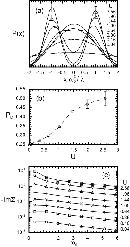
FIG. 1.: Results for the dispersionless model with $\omega_{0}=0.5$ at $\beta=8$; (a) the probability function of the boson fields $x$, (b) the probability of the double occupancy, and (c) the imaginary part of the self-energy for fermion as a function of Matsubara frequency. In (a), the typical errorbars are shown at the peaks of the distributions. The lines in (b) and (c) are guides to eye.

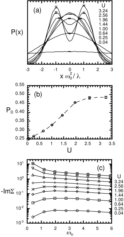
FIG. 2.: Results for the dispersionless model with $\omega_{0}=2$.

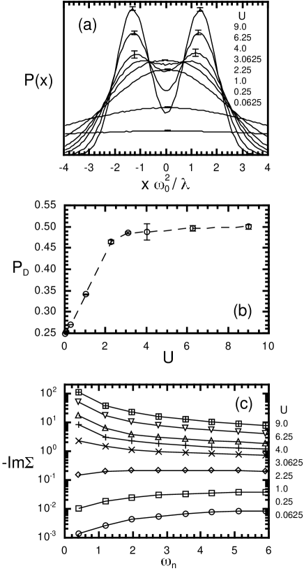
FIG. 3.: Results for the dispersionless model with $\omega_{0}=8$.

FIG. 4.: Results for the dispersive boson model in the weak coupling regime with $\omega_{0}=0.5$ and $U=0.16$ ($\lambda=0.2$) at $\beta=8$; (a) the bare impurity Green’s function for boson as a function of Matsubara frequency, (b) the imaginary part of the self-energy for fermion, and (c) the probability of the double occupancy as a function of the width of the boson dispersion. The lines are guides to eye.

FIG. 5.: Results for the dispersive boson model in the atomic regime with $\omega_{0}=8$ and $U=9$ ($\lambda=24$) at $\beta=8$; (a) the bare impurity Green’s function for boson at zero Matsubara frequency and (b) the imaginary part of the self-energy for fermion at the smallest Matsubara frequency. The lines are guides to eye.

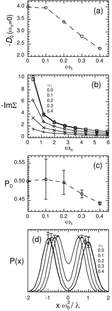
FIG. 6.: Results for the dispersive boson model with $\omega_{0}=0.5$ and $U=2.56$ ($\lambda=0.8$) at $\beta=8$; (a) the bare impurity Green’s function for boson at zero Matsubara frequency, (b) the imaginary part of the self-energy for fermion, (c) the probability of the double occupancy, and (d) the probability function of the boson fields $x$. The lines in (a)-(c) are guides to eye. In (d), the typical errorbars are shown at the peaks of the distributions.

FIG. 7.: Crossover in the intermediate coupling region with $\omega_{0}=0.5$ and $U=0.64$ ($\lambda=0.4$) at $\beta=8$; (a) the bare impurity Green’s function for boson at zero Matsubara frequency, (b) the imaginary part of the self-energy for fermion, and (c) the probability of the double occupancy. The lines are guides to eye.

FIG. 8.: The effective frequency of boson in the case of $\omega_{0}=0.5$ and $U=0.64$ at $\beta=8$. The line is a guide to eye.

FIG. 9.: The softening of the effective boson frequency for (a) $\omega_{0}=0.5$ and (b) $\omega_{0}=2.0$ at $\beta=8$. The lines are guides to eye.

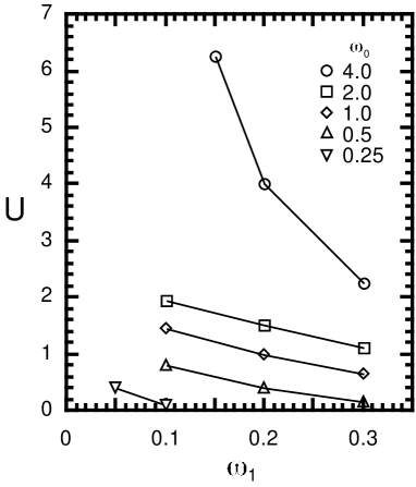
FIG. 10.: The phase diagram of the crossover for various values of $\omega_{0}$. The boundaries are determined by the complete softening of the effective boson frequency. The lines are guides to eye.

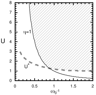
FIG. 11.: Schematic phase diagram for the dispersionless case. The critical value for the formation of the small-polaron state $U^{*}$ is shown as the dotted gray line. The solid line indicates the boundary $\eta=1$. The hatched area is the strong fluctuation region. See the text for details.

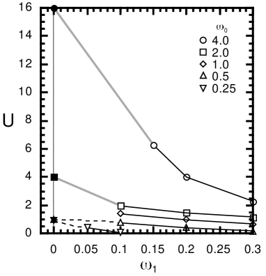
FIG. 12.: The values of $U$ and $\omega_{1}$ at which the crossover from the weak-fluctuation to the strong-fluctuation regime takes place. Notice that these values extrapolate smoothly to the values of $U$ at $\eta=1$ for $\omega_{0}=4$ and $2$ (anti-adiabatic regime) and to the $U^{*}$ for $\omega_{0}=0.5$ and $0.25$ (adiabatic regime) in the limit of $\omega_{1}=0$. See the text for details.

REFERENCES

- [1] G. D. Mahan, in Many Particle Physics, (Plenum Publishing, New York, 1981), and references therein.
- [2] J. Hubbard, Phys. Rev. Lett. 3, 77 (1959).
- [3] R. L. Stratonovich, Sov. Phys. Dokl. 2, 416 (1957).
- [4] A. B. Migdal, Zh. Eksp. Teor. Fiz. 34, 1438 (1958) [Sov. Phys. JETP 7, 996 (1958)].
- [5] T. Holstein, Ann. Phys. 8, 325 (1959).
- [6] T. Holstein, Ann. Phys. 8, 343 (1959).
- [7] A. Georges, G. Kotliar, W. Krauth, and M. J. Rozenberg, Rev. Mod. Phys. 68, 13 (1996), and references therein.
- [8] Q. Si, J. L. Smith, and K. Ingersent, cond-mat/9905006.
- [9] R. Chitra and G. Kotliar, cond-mat/9903180.
- [10] J. Robin, A. Romano, and J. Ranninger, cond-mat/9808252.
- [11] A. P. Ramirez, P. Schiffer, S.-W. Cheong, W. Bao, T. T. M. Palstra, P. L. Gammel, D. J. Bishop, and B. Zegarski, Phys. Rev. Lett. 76, 3188 (1996).
- [12] C. H. Chen, S.-W. Cheong, and H. Y. Hwang, J. Appl. Phys. 81, 4326 (1997).
- [13] S. Mori, C. H. Chen, and S.-W. Cheong, Nature (London) 392, 473 (1998).
- [14] M. T. Fernández-Díaz, J. L. Martínez, J. M. Alonso, and E. Herrero, Phys. Rev. B 59, 1277 (1999).
- [15] J. E. Hirsch and E. Fradkin, Phys. Rev. Lett. 49, 402 (1982).
- [16] J. E. Hirsch and E. Fradkin, Phys. Rev. B 27, 4302 (1983).
- [17] R. T. Scaletter, N. E. Bickers, and D. J. Scalapino, Phys. Rev. B 40, 197 (1989).
- [18] R. M. Noack, D. J. Scalapino, and R. T. Scaletter, Phys. Rev. Lett. 66, 778 (1991).
- [19] J. K. Freericks, M. Jarrell, and, D. J. Scalapino, Phys. Rev. B 48, 6302 (1993).
- [20] A. J. Millis, R. Mueller, and B. I. Shraiman, Phys. Rev. B 54, 5389 (1996).
- [21] J. E. Hirsch and R. M. Fye, Phys. Rev. Lett. 56, 2521 (1986).
- [22] K. Takegahara, J. Phys. Soc. Jpn. 62, 1736 (1992).
- [23] R. Micnus, J. Ranninger, and S. Robaszkiewics, Rev. Mod. Phys. 62, 113 (1990), and references therein.
- [24] P. G. J. van Dongen, Mod. Phys. Lett. B 5, 861 (1991).
- [25] P. G. J. van Dongen, Phys. Rev. B 45, 2267 (1992).
- [26] D. Feinberg, S. Ciuchi, and F. de Pasquale, Int. J. Mod. Phys. B 4, 1317 (1990).
- [27] M. Imada, A. Fujimori, and Y. Tokura, Rev. Mod. Phys. 70, 1039 (1998), and references therein.