The neutron resonance: modeling photoemission and tunneling data in the superconducting state of Bi₂Sr₂CaCu₂O_8+δ

Abstract

Motivated by neutron scattering data, we develop a model of electrons interacting with a magnetic resonance and use it to analyze angle resolved photoemission (ARPES) and tunneling data in the superconducting state of Bi₂Sr₂CaCu₂O_8+δ. We not only can explain the peak-dip-hump structure observed near the $(\pi,0)$ point, and its particle-hole asymmetry as seen in SIN tunneling spectra, but also its evolution throughout the Brillouin zone, including a velocity ‘kink’ near the d-wave node.

Recent advances in the momentum resolution of ARPES spectroscopy have led to a detailed mapping of the spectral lineshape in the high-T_c superconductor Bi₂Sr₂CaCu₂O_8+δ (BSCCO) throughout the Brillouin zone.[1, 2] In contrast to normal state data where well defined excitations do not exist, quasiparticle peaks were identified below $T_{c}$ along the entire Fermi surface.[3] Moreover, it has been known for some time that near the $(\pi,0)$ ($M$) point of the zone, the spectral function shows an anomalous lineshape, the so called ‘peak-dip-hump’ structure.[4, 5] The new data indicate a) near the d-wave node of the superconducting gap, the dispersion shows a characteristic ‘kink’ feature: for $|\omega|<\omega_{kink}$, the spectra exhibit sharp peaks with a weaker dispersion; above this, broad peaks with a stronger dispersion;[1, 2] b) away from the node, the dispersion kink develops into a ‘break’; the two resulting branches are separated by an energy gap, and overlap in momentum space; c) towards $M$, the break evolves into a pronounced spectral ‘dip’ separating the almost dispersionless quasiparticle branch from the weakly dispersing high energy branch (the ‘hump’); d) the kink, break, and dip features all occur at the same energy, independent of position in the zone.[1]

Features similar to the ARPES spectrum near the $M$ point were earlier observed in tunneling spectroscopy.[6] Experimental SIN junctions on BSCCO show a characteristic asymmetry, with a more pronounced dip-hump structure on the occupied side.[7] On the other hand, SIS junctions reveal a strong dip-hump feature on both bias sides.[8]

There have been several theoretical treatments which assigned the anomalous ARPES lineshape near the $M$ point of the zone to the coupling between spin fluctuations and electrons.[9, 10, 11, 12] Here, we are able to explain features a)-d) of the ARPES data, as well as the SIN tunneling asymmetry, in terms of the combined effect of A) the flat electronic dispersion near the $M$ point of the zone and B) coupling of the fermionic degrees of freedom to a bosonic mode which is sharp in energy and peaked in momentum near $\vec{Q}=(\pi,\pi)$. Our main result is that the anomalous features in the dispersion and lineshape for all points in the zone have the same origin.

A resonance mode with these characteristics is observed in inelastic neutron scattering experiments in bilayer cuprates in the superconducting state.[13, 14] The neutron resonance lies below a gapped continuum, the latter having a signal typically a factor of 30 less than the maximum at $\vec{Q}$ at the mode energy.[15] In order to extract the essential physics, we concentrate on the mode part and neglect the continuum. The latter contributes mainly to additional damping at higher energies. We treat the mode in a semi-phenomenological way, taking the relevant parameters from experiment. We then calculate the resulting electronic self energy to second order in the coupling constant. From the self energy we directly obtain the spectral function measured by ARPES, which we then use to calculate the tunneling conductance.

The retarded self energy on the real energy axis is given by[16]

$$\hat{\Sigma}^{R}=-\frac{ig^{2}}{2\mu_{B}^{2}}\hat{\tau}_{3}\left(\hat{G}^{K}*\chi^{R}+\hat{G}^{R}*\chi^{K}\right)\hat{\tau}_{3}$$ (1)

with $A*B(\vec{k},\epsilon)\equiv\sum_{\vec{q}}\int_{-\infty}^{\infty}\frac{d\omega}{2\pi}A(\vec{k}-\vec{q},\epsilon-\omega)B(\vec{q},\omega)$, $\hat{\tau}_{i}$ Pauli matrices in particle-hole space, and $g$ the effective coupling constant. The Keldysh ($K$) components are given in terms of retarded ($R$) and advanced ($A$) functions by $\hat{G}^{K}=(\hat{G}^{R}-\hat{G}^{A})(1-2f)$ and $\chi^{K}=(\chi^{R}-\chi^{A})(1+2b)$, with the usual Bose ($b$) and Fermi ($f$) distribution functions.

The model for the mode is based on measurements of the spin susceptibility from inelastic neutron scattering experiments.[14] The mode energy will be denoted by $\Omega$ and its energy width is assumed to be irrelevant for the self energy. This assumption will be confirmed later. This leads to the following model for the mode part of the susceptibility

$$\chi^{R/A}(\vec{q},\omega)=-f(\vec{q})\left(\frac{1}{\omega-\Omega\pm i\delta}-\frac{1}{\omega+\Omega\pm i\delta}\right)$$ (2)

Here $f(\vec{q})$ describes the momentum dependence of the mode and is assumed to be enhanced at the $(\pi,\pi)$ point. Using the correlation length $\xi$ we write it as

$$f(\vec{q})=\frac{\chi_{\vec{Q}}\xi^{-2}}{\xi^{-2}+4(\cos^{2}\frac{q_{x}}{2}+\cos^{2}\frac{q_{y}}{2})}$$ (3)

Experimentally the energy integrated susceptibility at the $(\pi,\pi)$ wavevector, $\pi\chi_{\vec{Q}}$, was determined to be $0.95\mu_{B}^{2}$ per plane for BSCCO,[14] leading to $\chi_{\vec{Q}}=0.3\mu_{B}^{2}$. For the correlation length, we take a conservative estimate of $\xi=2a$. This corresponds to a full width half maximum of $0.26$Å^-1, as observed in YBCO, but somewhat smaller than that estimated for BSCCO ($0.52$Å^-1)[14] which we feel is somewhat broad. The mode energy was chosen to be $\Omega=39$ meV, which represents the reported values between 35 and 43 meV.[14]

Though $\chi$ is ‘renormalized’, we use a bare $\hat{G}$ in Eq. 1. This is the same approximation as in Ref. [17], where it was shown that this is better than using renormalized $\hat{G}$ with vertex corrections neglected. This is unlike the electron-phonon problem, where Migdal’s theorem applies. We take the success of explaining the experimental features as strong support of this approximation.

The bare Green’s functions with normal state dispersion $\xi_{\vec{k}}$, gap function $\Delta_{\vec{k}}$, and excitation energy $E_{\vec{k}}=\sqrt{\xi_{\vec{k}}^{2}+\Delta_{\vec{k}}^{2}}$ are

$$\hat{G}^{R/A}(\vec{k},\epsilon)=\frac{\hat{\alpha}_{\vec{k}}}{\epsilon-E_{\vec{k}}\pm i\Gamma}+\frac{\hat{\beta}_{\vec{k}}}{\epsilon+E_{\vec{k}}\pm i\Gamma}$$ (4)

where $\alpha_{11}=(1+\xi_{\vec{k}}/E_{\vec{k}})/2$, $\beta_{11}=(1-\xi_{\vec{k}}/E_{\vec{k}})/2$, $\alpha_{12}=-\beta_{12}=-\Delta_{\vec{k}}/2E_{\vec{k}}$, etc. For the normal state dispersion we use a six-parameter tight binding fit.[18] We neglect bilayer splitting, as experiments suggest it is absent in BSCCO.[5] A characteristic feature of this dispersion is a flat band with a saddlepoint at $M$ with energy $\xi_{M}=-$34 meV. The superconducting gap function is taken to be the d-wave $\Delta_{\vec{k}}=\Delta_{0}(\cos k_{x}-\cos k_{y})/2$ with a maximal gap value of $\Delta_{0}=35$ meV. We have chosen $\Gamma=5$ meV as an intrinsic lifetime broadening. The coupling constant relevant for our model is $g^{2}\chi_{\vec{Q}}$, chosen to be 0.125 $\mbox{eV}^{2}\mu_{B}^{2}$. Given a value $\chi_{\vec{Q}}=0.3\mu_{B}^{2}$, this corresponds to $g=0.65$ eV, the same value as used in previous spin fluctuation work.[19] We performed the $\omega$-integration in Eq. 1 analytically and the correlation product in momentum space via fast Fourier transform, using $256\times 256$ points in the Brillouin zone.

In Fig. 1 we show the renormalization function $Z(\epsilon)=1-\Sigma_{0}(\epsilon)/\epsilon$, where $\Sigma_{0}$ is the $\hat{\tau}_{0}$ component of the $\hat{\Sigma}$ matrix. Since the $\vec{q}$ integral in Eq. 1 is dominated by the regions around the $M$ point where the band is flat and close to the chemical potential, there are features in the imaginary part of the self-energy connected with the two extremal energies $\Delta_{0}$ and $E_{M}=\sqrt{\xi_{M}^{2}+\Delta_{0}^{2}}$. These features do not show dispersion, but a change in magnitude with position in the zone which is determined by the momentum width of the mode. This is the central result of this paper. More generally, the imaginary part of the self energy is enhanced between the values

FIG. 1.: Renormalization function $Z(\epsilon)$ at the $M$=$(\pi,0)$ point (solid line) and at the node $(0.36\pi,0.36\pi)$ (dashed line) for $T=40$K.

$\epsilon_{1}=\Delta_{0}+\Omega$ and $\epsilon_{2}=E_{M}+\Omega$. For $\xi_{M}$ approaching the chemical potential, $E_{M}$ approaches $\Delta_{0}$ resulting in a peak-like feature in the self energy. For our case, $\epsilon_{1}=74$ meV and $\epsilon_{2}=88$ meV. Because the spectral weight of the mode is maximal near $\vec{Q}=(\pi,\pi)$, the $M$ points of the zone, which are connected by $\vec{Q}$, benefit mostly. This results in stronger features in the self energy near the $M$ points compared to e.g. the nodal points. The peaked structure in the imaginary part of the self energy results (via Kramers-Kronig relations) in an enhancement of the real part of the renormalization function for $|\epsilon|<\epsilon_{1}$, and a reduction of it for $|\epsilon|>\epsilon_{2}$, as shown in Fig. 1. This leads to a renormalization of the low-energy dispersion of the spectra compared to the high energy part. Since the experimental energy width of the neutron resonance is smaller than the variation in energy of typical features in the self energy, this confirms our assumption that the energy width of the mode is not relevant.

The spectral function is obtained by

$$A(\vec{k},\epsilon)=-2\mbox{Im}\left[\left(\hat{G}^{R}(\vec{k},\epsilon)^{-1}-\hat{\Sigma}^{R}(\vec{k},\epsilon)\right)^{-1}\right]_{11}$$ (5)

In Fig. 2 we show the spectral functions for momentum cuts through the $M$ point towards $Y=(\pi,\pi)$ ($MY$ cut), and parallel to $MY$ through the nodal point. Due to particle-hole coherence factors, there are quasiparticle peaks at $M$ on both sides of the chemical potential. On the negative energy side, the peak is more pronounced since $\xi_{M}$ is negative, and a strong dip feature is present. The asymmetry of the dip feature is a combined effect of the $\hat{\tau}_{3}$ component of $\hat{\Sigma}$, which introduces particle-hole asymmetry, and the inherent particle-hole asymmetry of the band structure near the $M$ point. Going from $M$ towards the Fermi surface (Fig. 2, bottom), the hump feature quickly loses weight as observed in ARPES.[1]

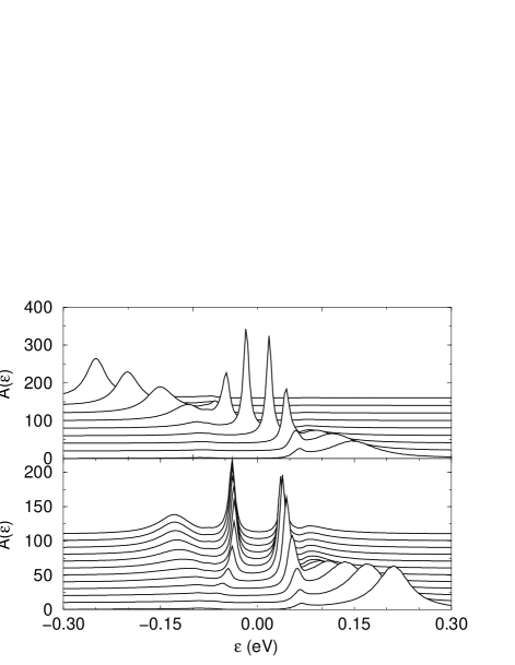
FIG. 2.: Spectral function $A(\vec{k},\epsilon)$ for $T=40$K. Top panel: for $\vec{k}$ points along the cut parallel to $MY$ through the order parameter node, from $(0.20\pi,0.36\pi)$ to $(0.51\pi,0.36\pi)$. Bottom panel: for $\vec{k}$ points along the $MY$ cut from $(0,\pi)$ to $(0.43\pi,\pi)$.

In the top panel of Fig. 2 we show spectra for a cut parallel to $MY$ through the order parameter node at the Fermi surface. Near the node there is only one peak crossing the chemical potential. The dip-hump features are very weak near the node and are presumably overshadowed by the additional lifetime effects due to the continuum part of the spin susceptibility. Note the much broader peaks for higher energies, $|\epsilon|>80$ meV, compared to the sharper peaks near the chemical potential, as observed in ARPES experiments.[1, 2, 3]

In Fig. 3 we present our results for the dispersion obtained from the maxima of the occupied part of the spectral function, $A(\vec{k},\epsilon)f(\epsilon)$. Near the $M$ point we observe an almost dispersionless strong peak feature at roughly the gap energy $-\Delta_{0}$, and a weaker hump feature at slightly below $-\epsilon_{2}$, consistent with experimental finding c). The peak feature, which without interaction with the mode would be at $E_{M}$, is pushed towards the chemical potential, thus ending up close to $\Delta_{0}$ for not too small coupling constants. The position of the hump feature is strongly dependent on the coupling constant. We adjusted $g$ to reproduce the experimental value of about -130 meV for the hump feature at $M$; this choice also results in the weak dispersion of the hump feature as observed in experiment.[1] As one goes away from $M$, the dispersion of the hump extents further below $-\epsilon_{2}$ and the peak starts to show dispersion, until a characteristic break in the dispersion with a jump at $\sim$-80 meV develops. This is exactly the experimental finding in point b). Note the stability of the characteristic -80 meV energy value for the break/dip feature throughout the zone. This is a result of the dominance of the region near $M$ in the $\vec{q}$ sum in Eq. 1, which sets the energy scale. Thus we confirm point d) of the experimental findings.

FIG. 3.: Calculated dispersion at $T=40$K obtained from the maxima of the occupied part of the spectral function for cuts along $k_{x}$ for fixed $k_{y}$ as indicated. Momenta are in units of $\pi$. The size of the symbols represents the peak intensity. The coupling constant is $g=0.65$ eV except in panel 1, where we show for comparison with panel 2 results for $g=0.39$ eV. Note striking similarity of this plot to the data of Ref. [1].

As the nodal point is approached, the self energy becomes weaker due to the momentum dependence of the mode. The sudden change in the linewidth for a cut parallel to $MY$ through the node (panel 2 of Fig. 3), as discussed in Fig. 2, occurs around -80 meV, in accordance with point a). We still observe a weak break feature, which will be smeared out by additional lifetime broadening from the continuum part of the susceptibility. This weak break is also reduced for a smaller coupling (panel 1), or if the Lorentzian in Eq. 3 is replaced by a Gaussian. Note that in accordance with experiments, the velocity near the nodal point is reduced compared to that for higher binding energies, causing a velocity ‘kink’.

Knowing the spectral function throughout the zone, we are able to calculate the tunneling spectra given a tunneling matrix element $T_{\vec{k}\vec{p}}$. From the SIN tunneling current $I(V)$ one obtains the differential conductance, $dI/dV$. As usual we neglect the energy dependence of the SIN matrix element $|M_{\vec{k}}|^{2}=2e\sum_{\vec{p}}|T_{\vec{k}\vec{p}}|^{2}A_{N}(\vec{p},\epsilon)$, where $A_{N}$ is the spectral function of the normal metal. The SIN tunneling current is then given by

$$I(V)=\sum_{\vec{k}}|M_{\vec{k}}|^{2}\int_{-\infty}^{\infty}\frac{d\epsilon}{2\pi}A(\vec{k},\epsilon)\left\{f(\epsilon)-f(\epsilon+eV)\right\}$$ (6)

In the top panels of Fig. 4, we show results for the SIN $dI/dV$ for several coupling strengths. We model the tunneling matrix element for two extreme cases: for incoherent tunneling we assume a constant $|M_{\vec{k}}|^{2}=M_{0}^{2}$, whereas for coherent tunneling we use $|M_{\vec{k}}|^{2}=\frac{1}{4}M_{1}^{2}(\cos k_{x}-\cos k_{y})^{2}$.[20]

FIG. 4.: Differential tunneling conductance for SIN (top) and SIS (bottom) tunnel junctions for $T=40$K. Units are $eM_{i}^{2}$ for SIN and $2e^{2}T_{i}^{2}$ for SIS. Left for isotropic tunneling ($i$=0), right for coherent tunneling ($i$=1). Curves are for $g$=0.39 eV (dotted), 0.65 eV (full line), and 0.90 eV (dashed).

In both cases, we observe a clear asymmetry with a dip-hump structure on the negative bias side and a very weak feature on the positive side of the spectrum, as in experiment [7]. The pronounced asymmetry is a result of the shallow band near the $M$ point, $\xi_{M}\sim-\Omega$, which enhances the coupling to the resonance mode for populated states. Note that the hump position is strongly dependent on the coupling constant in contrast to the position of the dip minimum. The asymmetry in the peak height on either side of the spectrum is sensitive to the coupling constant too. In weak coupling the negative bias peak is higher due to the Van Hove singularity at the $M$ point. For stronger coupling the pronounced dip at negative bias reduces the height of the coherence peak on this side and shifts the hump to higher energies. For $g$=$0.65$ eV (full lines in Fig. 4) the peaks at positive and negative bias have roughly the same height, as in experiment [7].

For an SIS junction, the single particle tunneling current is given in terms of the spectral functions by

$$I(V)=2e\sum_{\vec{k}\vec{p}}|T_{\vec{k}\vec{p}}|^{2}\int_{-\infty}^{\infty}\frac{d\epsilon}{2\pi}A(\vec{k},\epsilon)A(\vec{p},\epsilon+eV)$$ (7)

$$\times\left\{f(\epsilon)-f(\epsilon+eV)\right\}$$ (8)

Again we show results for incoherent tunneling ($|T_{\vec{k}\vec{p}}|^{2}=T_{0}^{2}$) and for coherent tunneling with conserved parallel momentum, $|T_{\vec{k}\vec{p}}|^{2}=\frac{1}{16}T_{1}^{2}(\cos k_{x}-\cos k_{y})^{4}\delta(\vec{k}_{||}-\vec{p}_{||})$.[20] We show the SIS $dI/dV$ in the bottom panels of Fig. 4. Our theoretical SIS curves for incoherent tunneling resemble very closely the experimental results for BSCCO,[8] unlike for coherent tunneling which exhibits negative $dI/dV$ regions due to the strong anisotropy of $T_{\vec{k}\vec{p}}$. Note that the dip-hump feature is strong on both sides for an SIS junction in contrast to the SIN results.

In conclusion, we have shown that the momentum dispersion of the ARPES spectra, as detailed in recent experiments, can be explained by a simple model which has as components A) a flat band region near the chemical potential in the normal state dispersion near the $(\pi,0)$ point of the zone; B) a nearly dispersionless bosonic mode which is peaked in momentum near the $(\pi,\pi)$ point, and which interacts with the fermionic degrees of freedom. The theoretical tunneling spectra obtained with the same parameter set are consistent with the experimental findings of an asymmetry of the peak-dip-hump structure in SIN tunneling spectra.

The authors would like to thank A. Kaminski and J.C. Campuzano for discussions concerning their photoemission data, and J. Zasadzinski concerning tunneling data. This work was supported by the U.S. Dept. of Energy, Basic Energy Sciences, under Contract No. W-31-109-ENG-38.

REFERENCES

- [1] A. Kaminski, et al., cond-mat/0004482 (2000).
- [2] P.V. Bogdanov, et al., cond-mat/0004349 (2000).
- [3] A. Kaminski, et al., Phys. Rev. Lett. 84, 1788 (2000).
- [4] D.S. Dessau, et al., Phys. Rev. Lett. 66, 2160 (1991).
- [5] H. Ding, et al., Phys. Rev. Lett. 76, 1533 (1996).
- [6] Q. Huang, et al., Phys. Rev. B 40, 9366 (1989).
- [7] Ch. Renner and Ø. Fischer, Phys. Rev. B 51, 9208 (1995).
- [8] D. Mandrus, et al., Nature (London) 351, 460 (1991).
- [9] T. Dahm, Phys. Rev. B 53, 14051 (1996); T. Dahm, D. Manske, and L. Tewordt, ibid. 54, 602 (1996).
- [10] Z.X. Shen and J.R. Schrieffer, Phys. Rev. Lett. 78, 1771 (1997).
- [11] M.R. Norman, et al., Phys. Rev. Lett. 79, 3506 (1997); M.R. Norman and H. Ding, Phys. Rev. B 57, R11089 (1998).
- [12] A. Abanov and A.V. Chubukov, Phys. Rev. Lett. 83, 1652 (1999) and Phys. Rev. B 61, R8241 (2000).
- [13] J. Rossat-Mignot, et al., Physica C 185-189, 86 (1991); H.A. Mook, et al., Phys. Rev. Lett. 70, 3490 (1993); H.F. Fong, et al., ibid. 75, 316 (1995).
- [14] H.F. Fong, et al., Nature (London) 398, 588 (1999); M. Boehm, et al., unpublished.
- [15] P. Bourges, in The gap symmetry and fluctuations in high superconductors, ed. J. Bok, et al. (Plenum, New York, 1998), p. 349.
- [16] J. Rammer and H. Smith, Rev. Mod. Phys. 58, 323 (1986).
- [17] Y.M. Vilk and A.-M.S. Tremblay, J. Phys. France 7, 1309 (1997).
- [18] M.R. Norman, et al., Phys. Rev. B 52, 615 (1995); parameters used here are (eV): =0.0989, =-0.5908, =0.0962, =-0.1306, =-0.0507, =0.0939.
- [19] P. Monthoux and D. Pines, Phys. Rev. B 49, 4261 (1994).
- [20] S. Chakravarty, et al., Science 261, 337 (1993).