Resistivity of a Metal between the Boltzmann Transport Regime and the Anderson Transition

Abstract

We study the transport properties of a finite three dimensional disordered conductor, for both weak and strong scattering on impurities, employing the real-space Green function technique and related Landauer-type formula. The dirty metal is described by a nearest neighbor tight-binding Hamiltonian with a single s-orbital per site and random on-site potential (Anderson model). We compute exactly the zero-temperature conductance of a finite-size sample placed between two semi-infinite disorder-free leads. The resistivity is found from the coefficient of linear scaling of the disorder-averaged resistance with sample length. This “quantum” resistivity is compared to the semiclassical Boltzmann expression computed in both Born approximation and multiple scattering approximation.

Ever since Anderson’s seminal paper, [1] a prime model for the theories of the disorder induced metal-insulator, or localization-delocalization [2] (LD), transition in non-interacting electron systems has been the tight-binding Hamiltonian (TBH) on a hypercubic lattice

$$\hat{H}=\sum_{\bf m}\varepsilon_{\bf m}|{\bf m}\rangle\langle{\bf m}|+t\sum_{\langle{\bf m},{\bf n}\rangle}|{\bf m}\rangle\langle{\bf n}|,$$ (1)

with nearest neighbor hopping matrix element $t$ between s-orbitals $\langle{\bf r}|{\bf m}\rangle=\psi({\bf r}-{\bf m})$ on adjacent atoms located at sites ${\bf m}$ of the lattice. The disorder is simulated by taking random on-site potential such that $\varepsilon_{\bf m}$ is uniformly distributed in the interval [-W/2,W/2]. This is commonly called the “Anderson model”. There are many numerical studies [3] of the LD transition, which occurs in three-dimensions (3D) for a half-filled band at the critical disorder strength [4] $W_{c}\approx 16.5t$. Experiments on real metals with strong scattering or strong correlations often yield resistivities which are hard to analyze. Theory gives guidance in two extreme regimes: (a) the semiclassical case where quasiparticles with definite ${\bf k}$ vector justify a Boltzmann approach and “weak localization” (WL) correction, [5] and (b) a scaling regime [6] near the LD transition to “strong localization”. Lacking a complete theory it is often assumed that the two limits join smoothly with nothing between. Experiments, however, are very often in neither extreme limit. The middle is wide and needs more attention.

Here we give a 3D numerical analysis focused not on the transition itself but instead on the resistivity for $1<W/t<W_{c}/t$; specifically we ask how rapidly does the resistivity $\rho(W)$ deviate from the values predicted by the usual Boltzmann theory valid when $W\ll t$. It has long been assumed that “Ioffe-Regel condition” [7] $\ell\sim 1/k_{F}\sim a$ ($\ell$ being the mean free path, and $a$ being the lattice constant) gives the criterion for sufficient disorder to drive the metal into an Anderson insulator. Figure 1 shows that this is wrong. By $W/t\sim 4$, where $\ell$ is close to $a$, there is little sign of a divergence away from the semiclassical extrapolation, and the LD transition is postponed to much larger values of $W/t$.

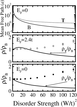
FIG. 1.: Resistivity $\rho$ at $E_{F}=0$ (lower panel) and $E_{F}=2.4t$ (middle panel), from a sample of cross section $A=225\,a^{2}$, normalized to the semiclassical Boltzmann resistivity $\rho_{\text{B}}$ calculated in the Born approximation. Also plotted are the ratios of $\rho_{\text{B}}$ to the Boltzmann resistivity $\rho_{\bf T}$ obtained using a ${\bf T}$-matrix for multiple scattering on a single impurity. The upper panel shows putative mean free paths obtained from $\rho_{\text{B}}$ (labeled by B) or $\rho_{\bf T}$ (labeled by T). Error bars at small $W/t$ are smaller than the size of the dot.

A cleaner discussion is possible using Kubo theory, which does not define $\ell$, but allows a definition of the diffusivity $D_{i}$ of an eigenstate $|i\rangle$, as shown below in Eq. (3). In the semiclassical regime, $D_{i}\rightarrow D_{k}=v_{k}\ell_{k}/3$. The diffusivity $D_{k}$ diminishes as $(W/t)^{-2}$ in Boltzmann theory. As $\ell/a$ approaches a minimum value ($\sim 1$), $D_{i}$ decreases toward $D_{\text{min}}=ta^{2}/\hbar$, which can be regarded as a minimum metallic diffusivity below which localization sets in. But there is a wide range of $W/t$ over which $D_{i}\lesssim D_{\text{min}}$ and yet the Boltzmann scaling $D\sim(t/W)^{2}$ is approximately right. In this regime single particle eigenstates $|i\rangle$ are neither ballistically propagating nor are they localized. There is a third category: intrinsically diffusive. [12] A wave packet built from such states has zero range of ballistic motion but an infinite range of diffusive propagation. Such states are found not only in a narrow crossover regime but over a wide range of parameters physically accessible in real materials and mathematically accessible in models like the Anderson model. In this regime, there is not a simple scaling parameter nor a universal behavior. But the behavior is quite insensitive to a changes in Fermi energy $E_{F}$ or $k_{B}T$, and scales smoothly with $W/t$.

The traditional tool for computation of $\rho$ has been the Kubo formula, [8] originally derived for a system in the thermodynamic limit. In a basis of exact single particle electron state $|i\rangle$ of energy $\epsilon_{i}$, this can be written as

$$\sigma=\frac{1}{\rho}=\frac{e^{2}}{\Omega}\sum_{i}\left(-\frac{\partial f}{\partial\epsilon_{i}}\right)D_{i}=e^{2}N(E_{F})\bar{D},$$ (2)

where $\Omega$ is the sample volume, $f$ is the equilibrium Fermi-Dirac distribution, $N(E_{F})$ the density of states at $E_{F}$, $\bar{D}$ the mean diffusivity, and state diffusivity is given by

$$D_{i}=\pi\hbar\sum_{j}|\langle i|\hat{v}_{x}|j\rangle|^{2}\delta(\epsilon_{i}-\epsilon_{j})$$ (3)

where $\hat{\bf v}$ is the velocity operator. These formulas, while correct, are hard to use numerically. [9] Thanks to the recent advances in mesoscopic physics, [10] it is now apparent that the Landauer scattering approach [11] (or equivalent “mesoscopic” Kubo reformulation for the finite-size systems [13]) provides superior numerical efficiency when computing the transport properties of finite disordered conductors. It relates the conductance of a sample to its quantum-mechanical transmission properties. This formalism emphasizes the importance of taking into account the interfaces between the sample and the rest of the circuit. [14] Transport in the sample is phase-coherent (i.e. effectively occurring at zero temperature); the dissipation and thus thermalization of electrons (necessary for the establishment of steady state) takes place in other parts of the circuit.

Our principal result for the (quantum) resistivity of Anderson model, using Landauer-type approach, is shown on Fig. 1 for two different Fermi energies $E_{F}=0$ (half-filled band) and $E_{F}=2.4t$ (approximately 70% filled band but falling somewhat as $W$, and thus the band-width, increases). The linearized Boltzmann equation $-e{\bf E}\cdot{\bf v}_{\bf k}\partial f/\partial\epsilon_{\bf k}=(dF_{\bf k}/dt)_{\text{scatt}}$ serves as a reference theory. Here $\epsilon_{\bf k}$ is the energy band for $W=0$, namely $\epsilon_{\bf k}=2t\sum\cos k_{\alpha}$, $\hbar v_{k\alpha}$ is $\partial\epsilon/\partial k_{\alpha}$, and $F_{\bf k}$ is the non-equilibrium distribution. The collision integral is

$$\left(\frac{dF}{dt}\right)_{\text{scatt}}=-\frac{2\pi}{\hbar}\sum_{{\bf k}^{\prime}}|V_{{\bf kk}^{\prime}}|^{2}(F_{\bf k}-F_{{\bf k}^{\prime}})\delta(\epsilon_{\bf k}-\epsilon_{\bf k^{\prime}}).$$ (4)

The mean squared matrix element of the random potential $|V_{{\bf kk}^{\prime}}|^{2}$, in Born approximation, is $\overline{\varepsilon^{2}_{\bf m}}=W^{2}/12$, where $\overline{(\ldots)}$ denotes average over probability distribution $P(\varepsilon_{\bf m})=(1/W)\theta(W/2-|\varepsilon_{\bf m}|)$. This equation assumes that quasiparticles propagate with mean free path $\ell>a$ between isolated collision events. The equation is exactly solvable, yielding (for $k_{B}T\ll t$) $1/\rho_{\text{B}}=e^{2}\tau(n/m)_{\text{eff}}$, with $(n/m)_{\text{eff}}=\sum v_{kx}^{2}\delta(\epsilon_{k}-E_{F})/\Omega$, and $\hbar/\tau=2\pi N(E_{F})W^{2}/12$. We have evaluated $(n/m)_{\text{eff}}$ and $N(E_{F})$ numerically. To within factors of order one, the Boltzmann-Born answer for the semiclassical resistivity is $\rho_{\text{B}}=(\pi\hbar a/e^{2})(W/4t)^{2}$. When $W=3t$ and $a=3{\text{\AA}}$, $\rho_{\text{B}}$ is $125\,\mu\Omega$cm, typical of dirty transition metal alloys, and close to the largest resistivity normally seen in dirty “good” metals. Figure 1 plots $\rho/\rho_{\text{B}}$ versus $(W/t)^{2}$. Even for $W=10t$ there is less than a factor of 2 deviation from the (unwarranted) extrapolation of the Boltzmann theory into the regime $W>t$. Boltzmann theory can be “improved” by including multiple scattering from single impurities, that is, replacing the impurity potential by the ${\bf T}$-matrix ${\bf T}_{\bf m}(z)=\varepsilon_{\bf m}/(1-\varepsilon_{\bf m}g(z))$ where $g(z)=(1/N_{s})\sum(z-\epsilon_{\bf k})^{-1}$ is the free particle Green function ($N_{s}$ is the number of lattice sites). To next order the mean square ${\bf T}$-matrix is

$$\overline{|{\bf T}_{\bf m}(z)|^{2}}=\frac{W^{2}}{12}\left(1+\frac{3W^{2}}{20t^{2}}(gg^{*}+gg+g^{*}g^{*})+\ldots\right),$$ (5)

where the first term is the Born approximation and the coefficient of the correction ($\sim{\mathcal{O}}(W^{4})$) changes sign from negative to positive as $E_{F}$ moves from 0 to $2.4t$. As shown on Fig. 1, the resistivity does not behave like $\overline{|{\bf T}_{\bf m}(z)|^{2}}$; multiple scattering with interference from pairs of impurities is at least equally important, and the “exact” $\rho(W)$ is less sensitive to details like $E_{F}$ than is the ${\bf T}$-matrix approximation. The rest of the paper presents the method of calculation and describes a bit of mesoscopic physics of very dirty metals.

The central linear transport quantity in the mesoscopic view, [2] as well as in the scaling theory of localization, [6] is conductance $G$ rather than conductivity $\sigma(L)=L^{2-d}G(L)$ (the bulk conductivity is an intensive material constant defined only in the thermodynamic limit, $\sigma=\lim_{L\rightarrow\infty}L^{2-d}G(L)$). We use a Landauer-type formula to get the exact quantum conductance $G$ of finite samples with disorder configurations chosen by a random number generator. Finite-size samples permit exact solutions for any strength of disorder. Similar to other recent works, [15, 16] the bulk resistivity is extracted from the disorder-averaged resistance $\langle R\rangle$ by finding the linear (Ohmic) scaling of $\langle R\rangle$ versus the length of the sample $L$ at fixed cross section $A$ (Fig. 2). Two kinds of errors [16] may arise: (a) The transition from the Ohmic regime to the localized regime occurs for length of the sample $L\sim\xi$ which happens when [17] $G={\mathcal{O}}(2e^{2}/h)$. If $L$ is made large enough, $G$ will always diminish to this magnitude. Therefore, we avoid using the sample sizes with too small $G$. (b) Finite-size boundary conditions and non-specular reflection [18] cause density of states and scattering properties of the sample to be slightly altered as compared to the true bulk. We expect these effects to be small for our samples where $\ell$ is smaller than the transverse size $\sqrt{A}$.

A two probe measuring configuration is used for computation. The sample is placed between two disorder-free ($\varepsilon_{\bf m}=0$) semi-infinite leads connected to macroscopic reservoirs which inject thermalized electrons at electrochemical potential $\mu_{L}$ (from the left) or $\mu_{R}$ (from the right) into the system. The electrochemical potential difference $eV=\mu_{L}-\mu_{R}$ is measured between the reservoirs. The leads have the same cross section as the sample. The hopping parameter in the lead and the one which couples the lead to the sample are equal to the hopping parameter in the sample. Thus, extra scattering (and resistance) at the sample-lead interface is avoided but transport at Fermi energies $|E_{F}|$ greater than the clean-metal band edge $|E_{b}|=6t$ cannot be studied. [9] Hard wall boundary conditions are used in the $\hat{y}$ and $\hat{z}$ directions. The sample is modeled on a cubic lattice with $N\times N_{y}\times N_{z}$ sites, where $N_{y}=N_{z}=15$ and lengths $L=Na$ are taken from the set $N\in\{5,10,15,20\}$.

The linear conductance is calculated using an expression obtained from the Keldysh technique [19]

$$G=\frac{4e^{2}}{\pi\hbar}\,\text{Tr}\left(\text{Im}\,\hat{\Sigma}_{L}\,\hat{G}^{r}_{1N}\,\text{Im}\,\hat{\Sigma}_{R}\,\hat{G}^{a}_{N1}\right).$$ (6)

Here $\text{Im}\,\hat{\Sigma}_{L,R}=(\hat{\Sigma}_{L,R}^{r}-\hat{\Sigma}_{L,R}^{a})/2i$ are self-energy matrices ($r$-retarded, $a$-advanced) which describe the coupling of the sample to the leads, and $\hat{G}^{r}_{1N}$, $\hat{G}^{a}_{N1}$ are Green function matrices connecting the layer $1$ and $N$ of the sample: $\hat{G}^{r,a}=(E-\hat{H}-\hat{\Sigma}^{r,a})^{-1}$ ($\hat{G}^{a}=[\hat{G}^{r}]^{\dagger}$), with $\hat{\Sigma}^{r}=\hat{\Sigma}_{L}^{r}+\hat{\Sigma}_{R}^{r}$ ($\hat{\Sigma}^{a}=[\hat{\Sigma}^{r}]^{\dagger})$. The self-energy matrices introduced by the leads are non-zero only on the end layers of the sample adjacent to the leads. They are given [10] by $\hat{\Sigma}^{r}_{L,R}({\bf n},{\bf m})=t^{2}\hat{g}_{L,R}^{r}({\bf n}_{S},{\bf m}_{S})$ with $\hat{g}_{L,R}^{r}({\bf n}_{S},{\bf m}_{S})$ being the surface Green function [13] of the bare semi-infinite lead between the sites ${\bf n}_{S}$ and ${\bf m}_{S}$ in the end atomic layer of the lead (adjacent to the corresponding sites ${\bf n}$ and ${\bf m}$ inside the conductor). Positive definiteness of the operators $-2\,\text{Im}\,\hat{\Sigma}_{L,R}$ makes it possible to find their square root and recast the expression under the trace of Eq. (6) as a Hermitian operator. The expression (6) then looks like the Landauer formula involving the transmission matrix ${\bf t}$

$$G = \frac{e^{2}}{\pi\hbar}\,\text{Tr}\,({\bf tt}^{{\dagger}})=\frac{e^{2}}{\pi\hbar}\sum_{n=1}^{N_{y}N_{z}}T_{n},$$ (7)

$${\bf t} = 2\sqrt{-\text{Im}\,\hat{\Sigma}_{L}}\,\hat{G}^{r}_{1N}\sqrt{-\text{Im}\,\hat{\Sigma}_{R}},$$ (8)

or transmission eigenvalues $T_{n}$ when the trace is evaluated in a basis which diagonalizes ${\bf tt}^{{\dagger}}$.

For the case of two probe geometry the average transmission in the semiclassical transport regime ($a<\ell\ll L\ll\xi$) is given by [10] $\langle T\rangle=\ell_{0}/(\ell_{0}+L)$, with $\ell_{0}$ being of the order of $\ell$.

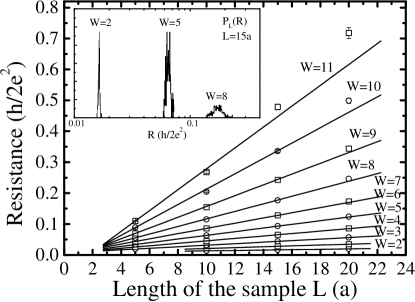
FIG. 2.: Linear fit $\langle R\rangle=C_{1}+\rho\,L/A$, ($A=225\,a^{2}$) for the disorder-averaged resistance $\langle R\rangle$ in the band center $E_{F}=0$ and different disorder strengths $W$. The intercept $C_{1}$ is decreasing with increasing $W$ (i.e. it is not determined just by the contact resistance $\pi\hbar/147e^{2}$) and becomes negative for $W\gtrsim 7t$. The inset shows examples of the distribution of resistances $P_{L}(R)$ (for $L=15a$) versus $\log R$. The distribution broadens either by increasing $W$ or the length of the sample (the units on the $y$-axis are arbitrary and different for each distribution).

Thus, the semiclassical limit [20] of the Landauer formula for conductance $\langle G\rangle=(e^{2}/\pi\hbar)\,M\langle T\rangle$ (measured between points deep inside the reservoirs) in the case of not too strong scattering should have the form

$$\langle G\rangle^{-1}=R_{C}+\rho\frac{L}{A}.$$ (9)

It describes the (classical) series addition of two resistors. The “contact” resistance [21] $R_{C}=\pi\hbar/e^{2}M$ is non-zero, even in the case of ballistic transport when the second term containing the resistivity $\rho=(\pi\hbar/e^{2})\,A/\ell_{0}M$ vanishes. Here $M\sim k_{F}^{2}A$ is the number of propagating transverse modes at $E_{F}$, also referred to as “channels”. A ballistic conductor with a finite cross section can carry only finite currents (the voltage drop occurs at the lead-reservoir interface). Using this simple analysis for guidance, we plot average resistances (taken over $N_{\text{conf}}=200$ realization of disorder) versus $L$ in Fig. 2, and fit with the linear function

$$\langle R\rangle=C_{1}+C_{2}L,\ C_{2}=\rho/A.$$ (10)

The resistivity $\rho$ on Fig. 1 is obtained from the fitted value of $C_{2}$. For very small values of $W$ the constant $C_{1}$ is approximately equal to $R_{C}=\pi\hbar/e^{2}M$ (where $M=147$ is the number of open channels in the band center). To our surprise, $C_{1}$ diminishes steadily with increasing $W$, and even turns negative around $W\gtrsim 7t$.

The quantum conductance $G$ fluctuates from sample to sample exhibiting universal conductance fluctuations [22] (UCF) $\Delta G=\sqrt{\text{Var}\,G}\simeq e^{2}/\pi\hbar$ in the semiclassical transport regime $G\gg e^{2}/\pi\hbar$. The inset on Fig. 2 shows the distribution of resistance [23] $P_{L}(R)$ for our numerically generated impurity ensemble. The error bars, used as weights in the fit (10), are computed as $\delta\langle R\rangle=\sqrt{\text{Var}R/N_{\text{conf}}}$. We find that $\Delta G$ is indeed independent of the size $L$ (of cubic samples), but decreases systematically by a factor $\approx 3$ as $W$ increases to the critical value $W_{c}$ (Fig. 3). On the other hand, $\Delta R$, being similar to $\Delta G/G^{2}$, depends on sample size. As $W$ approaches $W_{c}$, $G$ gets smaller until (for our finite samples) $\Delta G/G\sim 1$. At this point the distribution of resistances $R=1/G$ becomes very broad and $\langle R\rangle$ begins to rise above $1/\langle G\rangle$. For $L=15$ this happens when $W\gtrsim 12t$. At large $W$ the conductance of long samples ($N=20$) becomes close to $e^{2}/\pi\hbar$ and deviations from Ohmic scaling are expected. Therefore, we do not use these points in the fitting procedure when $W\gtrsim 10t$ (keeping the conductance [16] of the fitted samples $G>2e^{2}/\pi\hbar$).

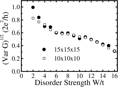
FIG. 3.: The conductance fluctuations ($\Delta G=\sqrt{\text{Var}\,G}$ at $E_{F}=0$) from weak to strong scattering regime in the disordered cubic samples $10\times 10\times 10$ and $15\times 15\times 15$.

We do not have a complete explanation for the deviation of $C_{1}$ (10) from the quantum point contact resistance $R_{C}$. In the semiclassical regime $G\gg e^{2}/\pi\hbar$ there are corrections to the Ohmic scaling $G\propto L^{d-2}$. The Diffuson-Cooperon diagrammatic perturbation theory gives a (negative) WL correction [5]

$$\sigma(L)=\sigma+\frac{e^{2}}{\pi^{2}\hbar 2\sqrt{2}}\frac{1}{L}-\frac{e^{2}}{\pi^{3}\hbar}\frac{1}{\ell_{0}^{\prime}},$$ (11)

where $\ell_{0}^{\prime}$ is a length of order $\ell$ (its precise value does not lead to observable consequences in the experiments studying WL, as long as it is unaffected by the temperature and the magnetic field). The positive $1/L$ term in Eq. 11 provides a possible picture for our finding that $C_{1}$in Eq. (10) goes negative as $W$ increases. However, this picture is an extrapolation from the semiclassical into the “middle” regime of intrinsically diffusive states, and therefore should be given little weight. The negative values of $C_{1}$ is better regarded as a new numerical result from the mesoscopic dirty metal theory.

It is interesting to note that in many $d$-band intermetallic compounds, $\rho$ “saturates” at a constant value [24] rather than following the semiclassical extrapolation, that is, increasing linearly with $T$ at high $T$. High $T_{c}$ materials and doped C₆₀ metals, on the other hand, do not saturate. [24] Within Boltzmann theory, the static disorder measured by $(W/t)^{2}$ plays the same role as thermal disorder or squared lattice displacement $\propto k_{B}T$. Our numerical results thus can be described as “failing to saturate.” Similar failure was seen in high $T$ Monte Carlo studies by Gunnarsson and Han. [25]

We thank I. L. Aleiner for interesting discussions and challenging questions. Suggestions provided by J. A. Vergés are acknowledged. This work was supported in part by NSF grant no. DMR 9725037.

REFERENCES

- [1] P. W. Anderson, Phys. Rev. 109, 1492 (1958).
- [2] M. Janssen, Phys. Rep. 295, 1 (1998).
- [3] B. Kramer and A. MacKinnon, Rep. Prog. Phys. 56, 1469 (1993).
- [4] K. Slevin, T. Ohtsuki, and T. Kawarabayashi, Phys. Rev. Lett, 84 3915 (2000).
- [5] L. P. Gor’kov, A. I. Larkin, D. E. Khmel’nitskii, Pis’ma Zh. Eksp. Teor. Fiz. 30, 248 (1979) [JETP Lett. 30, 228 (1979)].
- [6] E. Abrahams, P. W. Anderson, D. C. Licciardello, and T. V. Ramakrishnan, Phys. Rev. Lett. 42, 673 (1979).
- [7] A. F. Ioffe and A. R. Regel, Progr. Semicon. 4, 237 (1960).
- [8] R. Kubo, J. Phys. Soc. Jpn. 12, 570 (1957).
- [9] B. K. Nikolić and P. B. Allen, in preparation.
- [10] S. Datta, Electronic transport in mesoscopic systems (Cambridge University Press, Cambridge, 1995).
- [11] R. Landauer, IBM J. Res. Develop. 1, 223 (1957); Phil. Mag. 21, 863 (1970).
- [12] P. B. Allen, J. L. Feldman, J. Fabian, and F. Wooten, Phil. Mag. B 79, 1715 (1999).
- [13] J. A. Vergés, Comp. Phys. Comm. 118, 71 (1999).
- [14] Y. Imry and R. Landauer, Rev. Mod. Phys. 71, S306 (1999).
- [15] R. Kahnt, J. Phys. Condens. Matter 7, 1543 (1995).
- [16] T. N. Todorov, Phys. Rev. B 54, 5801 (1996).
- [17] D. J. Thouless, Phys. Rev. Lett 39, 1167 (1977).
- [18] E. H. Sondheimer, Adv. Phys. 1, 1 (1952).
- [19] C. Caroli, R. Combescot, P. Nozieres, and D. Saint-James, J. Phys C 4, 916 (1971).
- [20] H. U. Baranger, D. P. DiVincenzo, R. A. Jalabert, and A. D. Stone, Phys. Rev. B 44, 10 637 (1991).
- [21] Yu. V. Sharvin, Zh. Eksp. Teor. Fiz. 48, 984 (1965) [Sov. Phys. JETP 21, 655 (1965)].
- [22] B. L. Al’tshuler, Pis’ma Zh. Eksp. Teor. Fiz. 41 530 (1985) [JEPT Lett. 41, 648 (1985)]; P. A. Lee and A. D. Stone, Phys. Rev. Lett. 55, 1622 (1985).
- [23] A. Cohen, Y. Roth, and B. Shapiro, Phys. Rev. B 38, 12 125 (1988).
- [24] P.B. Allen, Comm. on Cond. Mat. Phys. 15, 327 (1992).
- [25] O. Gunnarsson and J. E. Han, Nature 405, 1027 (2000).