An exact-diagonalization study of rare events in disordered conductors

Abstract

We determine the statistical properties of wave functions in disordered quantum systems by exact diagonalization of one-, two- and quasi-one dimensional tight-binding Hamiltonians. In the quasi-one dimensional case we find that the tails of the distribution of wave-function amplitudes are described by the non-linear $\sigma$-model. In two dimensions, the tails of the distribution function are consistent with a recent prediction based on a direct optimal fluctuation method.

It is well established that disordered quantum systems in the metallic regime (i.e., in the limit of weak disorder) and highly excited classically chaotic quantum systems exhibit universal quantum fluctuations that can be described by random matrix theory (RMT): statistical properties, on the scale of the mean level spacing, of eigenvalues, eigenfunctions, and matrix elements are universal, i.e., they do not depend on the microscopic details of the systems under consideration [1, 2, 3, 4, 5].

However, in ballistic, classically chaotic quantum systems, non-hyperbolic phase-space structures may lead to deviations from universal RMT statistics [3]. Similarly fluctuations in disordered, classically diffusive quantum systems may deviate considerably from the RMT predictions due to increased localization. This effect is naturally very significant in the tails of distribution functions [6] (corresponding to rare events) of wave-function amplitudes [7, 8, 9, 10, 11, 12, 13], of the local density of states [7, 12], of inverse participation ratios [12, 13] and of NMR line shapes [7]. In all of these cases (with the exception of Ref. [7] which deals with one-dimensional (1D) systems), the distribution functions have been calculated using the non-linear $\sigma$-model (NLSM). Very recently, this approach has been extended to ballistic systems [14, 15] (see also [16, 17, 18]).

In Ref. [19] a direct optimal fluctuation method [20] was used to calculate the tails of distributions of current relaxation times and wave-function amplitudes; and predictions differing from [8, 9, 10, 11, 12, 13] were put forward. This led the authors of [19] to question the suitability of the NLSM to describe rare events in disordered conductors.

It is thus of great interest to test the predictions of [7, 8, 9, 10, 11, 12, 13] and [19] against results of independent calculations. In this letter, we have determined distribution functions of wave-function amplitudes by exact diagonalization of 1D, 2D and quasi-1D tight-binding Hamiltonians; in this case rare events correspond to unusually high splashes of wave-function amplitudes. We note that wave-function amplitude distributions can be measured in micro-wave experiments [21, 22].

We use the Anderson model of localization [23] which is a tight-binding model on a $d$-dimensional hyper-cubic lattice

$$\widehat{H}=\sum_{{\mathchoice{{\hbox{\boldmath$\displaystyle r$}}}{{\hbox{\boldmath$\textstyle r$}}}{{\hbox{\boldmath$\scriptstyle r$}}}{{\hbox{\boldmath$\scriptscriptstyle r$}}}},{\mathchoice{{\hbox{\boldmath$\displaystyle r$}}}{{\hbox{\boldmath$\textstyle r$}}}{{\hbox{\boldmath$\scriptstyle r$}}}{{\hbox{\boldmath$\scriptscriptstyle r$}}}}^{\prime}}t^{\phantom{\dagger}}_{{\mathchoice{{\hbox{\boldmath$\displaystyle r$}}}{{\hbox{\boldmath$\textstyle r$}}}{{\hbox{\boldmath$\scriptstyle r$}}}{{\hbox{\boldmath$\scriptscriptstyle r$}}}}{\mathchoice{{\hbox{\boldmath$\displaystyle r$}}}{{\hbox{\boldmath$\textstyle r$}}}{{\hbox{\boldmath$\scriptstyle r$}}}{{\hbox{\boldmath$\scriptscriptstyle r$}}}}^{\prime}}c_{\mathchoice{{\hbox{\boldmath$\displaystyle r$}}}{{\hbox{\boldmath$\textstyle r$}}}{{\hbox{\boldmath$\scriptstyle r$}}}{{\hbox{\boldmath$\scriptscriptstyle r$}}}}^{\dagger}\ c^{\phantom{\dagger}}_{{\mathchoice{{\hbox{\boldmath$\displaystyle r$}}}{{\hbox{\boldmath$\textstyle r$}}}{{\hbox{\boldmath$\scriptstyle r$}}}{{\hbox{\boldmath$\scriptscriptstyle r$}}}}^{\prime}}+\sum_{\mathchoice{{\hbox{\boldmath$\displaystyle r$}}}{{\hbox{\boldmath$\textstyle r$}}}{{\hbox{\boldmath$\scriptstyle r$}}}{{\hbox{\boldmath$\scriptscriptstyle r$}}}}{\upsilon}^{\phantom{\dagger}}_{\mathchoice{{\hbox{\boldmath$\displaystyle r$}}}{{\hbox{\boldmath$\textstyle r$}}}{{\hbox{\boldmath$\scriptstyle r$}}}{{\hbox{\boldmath$\scriptscriptstyle r$}}}}c_{\mathchoice{{\hbox{\boldmath$\displaystyle r$}}}{{\hbox{\boldmath$\textstyle r$}}}{{\hbox{\boldmath$\scriptstyle r$}}}{{\hbox{\boldmath$\scriptscriptstyle r$}}}}^{\dagger}c^{\phantom{\dagger}}_{\mathchoice{{\hbox{\boldmath$\displaystyle r$}}}{{\hbox{\boldmath$\textstyle r$}}}{{\hbox{\boldmath$\scriptstyle r$}}}{{\hbox{\boldmath$\scriptscriptstyle r$}}}}\,.$$ (1)

Here ${\mathchoice{{\hbox{\boldmath$\displaystyle r$}}}{{\hbox{\boldmath$\textstyle r$}}}{{\hbox{\boldmath$\scriptstyle r$}}}{{\hbox{\boldmath$\scriptscriptstyle r$}}}}=(x,y,\ldots)$ denotes sites on the lattice, $c_{\mathchoice{{\hbox{\boldmath$\displaystyle r$}}}{{\hbox{\boldmath$\textstyle r$}}}{{\hbox{\boldmath$\scriptstyle r$}}}{{\hbox{\boldmath$\scriptscriptstyle r$}}}}^{\dagger}$ and $c_{\mathchoice{{\hbox{\boldmath$\displaystyle r$}}}{{\hbox{\boldmath$\textstyle r$}}}{{\hbox{\boldmath$\scriptstyle r$}}}{{\hbox{\boldmath$\scriptscriptstyle r$}}}}$ are the usual creation and annihilation operators, the hopping amplitudes are $t_{{\mathchoice{{\hbox{\boldmath$\displaystyle r$}}}{{\hbox{\boldmath$\textstyle r$}}}{{\hbox{\boldmath$\scriptstyle r$}}}{{\hbox{\boldmath$\scriptscriptstyle r$}}}}{\mathchoice{{\hbox{\boldmath$\displaystyle r$}}}{{\hbox{\boldmath$\textstyle r$}}}{{\hbox{\boldmath$\scriptstyle r$}}}{{\hbox{\boldmath$\scriptscriptstyle r$}}}}^{\prime}}=1$ for nearest neighbour sites and zero otherwise. The on-site potential $\upsilon_{\mathchoice{{\hbox{\boldmath$\displaystyle r$}}}{{\hbox{\boldmath$\textstyle r$}}}{{\hbox{\boldmath$\scriptstyle r$}}}{{\hbox{\boldmath$\scriptscriptstyle r$}}}}$ is taken to be uncorrelated white noise, with zero mean and variance $\langle\upsilon_{\mathchoice{{\hbox{\boldmath$\displaystyle r$}}}{{\hbox{\boldmath$\textstyle r$}}}{{\hbox{\boldmath$\scriptstyle r$}}}{{\hbox{\boldmath$\scriptscriptstyle r$}}}}\upsilon_{{\mathchoice{{\hbox{\boldmath$\displaystyle r$}}}{{\hbox{\boldmath$\textstyle r$}}}{{\hbox{\boldmath$\scriptstyle r$}}}{{\hbox{\boldmath$\scriptscriptstyle r$}}}}^{\prime}}\rangle=\delta_{{\mathchoice{{\hbox{\boldmath$\displaystyle r$}}}{{\hbox{\boldmath$\textstyle r$}}}{{\hbox{\boldmath$\scriptstyle r$}}}{{\hbox{\boldmath$\scriptscriptstyle r$}}}}{\mathchoice{{\hbox{\boldmath$\displaystyle r$}}}{{\hbox{\boldmath$\textstyle r$}}}{{\hbox{\boldmath$\scriptstyle r$}}}{{\hbox{\boldmath$\scriptscriptstyle r$}}}}^{\prime}}W^{2}/12$. The parameter $W$ characterizes the disorder strength. As is well-known (see for instance [24, 25]), the eigenvalues $E_{j}$ and eigenfunctions $\psi_{j}({\mathchoice{{\hbox{\boldmath$\displaystyle r$}}}{{\hbox{\boldmath$\textstyle r$}}}{{\hbox{\boldmath$\scriptstyle r$}}}{{\hbox{\boldmath$\scriptscriptstyle r$}}}})$ of this Hamiltonian, in the metallic regime, exhibit fluctuations described by RMT. In this case, Dyson’s Gaussian orthogonal ensemble [1] is appropriate. When the matrix elements $t_{{\mathchoice{{\hbox{\boldmath$\displaystyle r$}}}{{\hbox{\boldmath$\textstyle r$}}}{{\hbox{\boldmath$\scriptstyle r$}}}{{\hbox{\boldmath$\scriptscriptstyle r$}}}}{\mathchoice{{\hbox{\boldmath$\displaystyle r$}}}{{\hbox{\boldmath$\textstyle r$}}}{{\hbox{\boldmath$\scriptstyle r$}}}{{\hbox{\boldmath$\scriptscriptstyle r$}}}}^{\prime}}$ of (1) are given an appropriate complex phase factor, Dyson’s unitary ensemble [1] applies. We refer to these two cases by assigning, as usual, the parameter $\beta=1$ to the former and $\beta=2$ to the latter. The metallic regime is characterized by $g\gg 1$ where $g=2\pi\nu VDL^{-2}$ is the dimensionless conductance (we take $\hbar=1$). Here $\nu=1/(V\Delta)$, $\Delta$ is the mean level spacing and $V$ the volume. $D=v_{\rm F}^{2}\tau/d$ is the diffusion constant, $\tau$ the mean free time and $v_{\rm F}$ the Fermi velocity. Four length scales are important: the lattice spacing $a$, the linear extension $L$, the localization length $\xi$ and the mean free path $\ell=v_{\rm F}\tau$.

By diagonalizing the Hamiltonian $\widehat{H}$ using a modified Lanczos algorithm [26], we have determined the distribution function

$$f_{\beta}(E,{\mathchoice{{\hbox{\boldmath$\displaystyle r$}}}{{\hbox{\boldmath$\textstyle r$}}}{{\hbox{\boldmath$\scriptstyle r$}}}{{\hbox{\boldmath$\scriptscriptstyle r$}}}};t)=\Delta\Big{\langle}\sum_{j}\!\delta(t\!-\!|\psi_{j}(\mathchoice{{\hbox{\boldmath$\displaystyle r$}}}{{\hbox{\boldmath$\textstyle r$}}}{{\hbox{\boldmath$\scriptstyle r$}}}{{\hbox{\boldmath$\scriptscriptstyle r$}}})|^{2}V)g_{\eta}(E\!-\!E_{j})\Big{\rangle}_{W}\,.$$ (2)

Here $\langle\cdots\rangle_{W}$ denotes an average over disorder realisations. The wave functions are normalized so that $\langle|\psi_{j}({\mathchoice{{\hbox{\boldmath$\displaystyle r$}}}{{\hbox{\boldmath$\textstyle r$}}}{{\hbox{\boldmath$\scriptstyle r$}}}{{\hbox{\boldmath$\scriptscriptstyle r$}}}})|^{2}\rangle_{W}=V^{-1}$ and $g_{\eta}(E)$ is a window function of width $\eta$, centered around $E=0$ and normalized to unity. In the following we describe the results of our calculations and compare them to the predictions of Refs. [8, 9, 10, 11, 12, 13, 19].

1D case. The eigenstates in a disordered chain are localized with localization length $\xi=4\ell$. According to Ref. [7] the distribution of wave-function amplitudes in a disordered chain of length $L$ is [27]

$$f(E;t)\simeq\frac{\xi}{Lt}\exp\Big{(}-\frac{t\,\xi}{L}\Big{)}$$ (3)

for $L\gg\ell$, independent of $x$ and $\beta$. Our results for $\langle f(E,x;t)\rangle_{x}$ ($\langle\cdots\rangle_{x}$ denotes an average over the $x$ coordinate) in Fig. 1 show very good agreement with Eq. (3) for large $L/\xi$. The deviations at small $t$ for $L/\xi=4.76$ are due to the fact that Eq. (3) is only valid asymptotically for large $L$. It does not take into account that in a system of finite length $L$, the smallest amplitude of a normalized, exponentially decaying wave function is of the order of $t_{\rm c}\simeq(L/\xi)\,\exp(-L/\xi)$. This cut-off is shown in Fig. 1.

Quasi-1D case. In this case, as was shown in Refs. [8, 9], the NLSM can be solved exactly for the distribution function $f_{\beta}(E,x;t)$, using a transfer matrix approach [28]. The result is [8, 9, 12, 13]

$$f_{1}(E,x;t)=\frac{2\sqrt{2}}{\pi\sqrt{t}}\frac{{\rm d}^{2}}{{\rm d}t^{2}}\int_{0}^{\infty}\!\frac{{\rm d}z}{\sqrt{z}}\,Y(z+t/2)\,,$$ (4)

$$f_{2}(E,x;t)=\frac{{\rm d}^{2}}{{\rm d}t^{2}}Y(t)\,.$$ (5)

Here $Y(z)={\cal W}(z\xi/L,x/\xi)\,{\cal W}(z\xi/L,(L-x)/\xi)$ and ${\cal W}(z,\tau)$ obeys the differential equation

$$\frac{\partial}{\partial\tau}{\cal W}(z,\tau)=\Big{(}z^{2}\frac{\partial^{2}}{\partial z^{2}}-z\Big{)}{\cal W}(z,\tau)$$ (6)

with initial condition ${\cal W}(z,0)=1$. The function ${\cal W}(z,t)$ may be determined in terms of an eigenfunction expansion of the operator $z^{2}\partial_{z}^{2}-z$ [9, 12, 13]. The change of the body and the tails of distribution $f_{\beta}(E,x;t)$ due to increasing localization may thus be parameterized by a single parameter which we define to be $X\equiv(\beta/2)L/\xi$. Here $\xi\equiv\beta\pi\nu DS$ where $S$ is the cross-section of the wire. Thus $X$ does not depend on $\beta$. In the metallic regime (where $X\rightarrow 0$) $Y(z)\simeq\exp(-z)$ which leads to the usual RMT results $f^{(0)}_{1}(t)=\exp(-t/2)/\sqrt{2\pi t}$ and $f^{(0)}_{2}(t)=\exp(-t)$. The former distribution ($\beta=1$) is often referred to as the Porter-Thomas distribution [2]. For increasing localization (finite but still small $X$), the ${\cal O}(X)$-corrections to the body of the distribution function $f^{(0)}_{\beta}$ are obtained by expanding $Y\simeq\exp(-t)[1+\beta^{-1}t^{2}P(x,x;0)]$ where $P(x,x^{\prime};\omega)$ is the one-dimensional diffusion propagator. The result is $f_{\beta}(E,x;t)=f^{(0)}_{\beta}(t)[1+\delta f_{\beta}(E,x;t)]$ with

$$\delta f_{\beta}(E,x;t)\! \simeq \!P(x,x;0)\!\left\{\begin{array}[]{ll}3/4\!-\!3t/2\!+\!t^{2}/4&\!\mbox{for$\,\beta\!=\!1$}\,,\\ 1\!-\!2t\!+\!t^{2}/2&\!\mbox{for$\,\beta\!=\!2$}\,,\end{array}\right.$$ (9)

valid for $t\ll X^{-1/2}$. In the tails ($t\gg X^{-1}>1$) of $f_{\beta}(E,x;t)$, Eqs. (4) and (5) simplify to [9]

$$f_{\beta}(E,x;t)\simeq A_{\beta}(x,X)\exp(-2\beta\sqrt{t/X})\,.$$ (10)

This result may also be obtained within a saddle-point approximation to the NLSM [10]. The prefactors $A_{\beta}(x,X)$ for $\beta=1,2$ are given in [9, 10].

According to Refs. [5, 28] and [8, 9, 10, 11, 12, 13] the NLSM applies provided the following conditions are satisfied:

$$1\ll k_{\rm F}\ell\ll k_{\rm F}^{2}S\ll k_{\rm F}L$$ (11)

where $k_{\rm F}$ is the Fermi wave vector and $S$ is the cross section of the wire. The first condition ensures that disorder is sufficiently weak. The second condition implies that apart from the sample geometry, all other properties are essentially 3D [28]. Due to the third condition the return probability is dominated by diffusive contributions [13]. When $k_{\rm F}={\cal O}(a^{-1})$, Eq. (11) corresponds to $1\ll\ell/a\ll M\ll L/a$, where $M=k_{\rm F}^{2}S$ is the number of channels. Furthermore, in the metallic regime, one must have $\ell\ll L\ll\xi$. Since $\xi\simeq M\ell$, this implies

$$1\ll L/\ell\ll M\,.$$ (12)

In a finite system, the conditions (11) and (12) are not easily met simultaneously. We have performed exact diagonalizations for $128\times 4\times 4$ and $128\times 8\times 8$ lattices, using open boundary conditions (BC) in the longitudinal direction. In this case, $P(x,x;0)=2X\,[1/3-x(L\!-\!x)/L^{2}]$.

The results of our calculations are summarized in Figs. 2 and 3. Figure 2 shows $\langle\delta f_{\beta}(E,x;t)\rangle_{x}$ in comparison with Eqs. (4),(5) and (9). We observe very good agreement. The value of $P\equiv\langle P(x,x;0)\rangle_{x}$ should be independent of $\beta$. As can be seen in Fig. 2, the value of $P$ does somewhat change with $\beta$, albeit weakly. For narrower wires ($128\times 4\times 4$) we have observed that the ratio $P_{1}/P_{2}$ (determined by fitting $P\equiv P_{\beta}$ independently for $\beta=1,2$) becomes very small for small values of $W$ (corresponding to $X\stackrel{{\scriptstyle<}}{{\sim}}0.1$) while it approaches unity for large values of $W$. A possible explanation for this deviation would be that for small $M$ and small $X$, the condition (11) is no longer satisfied since $\ell/a\stackrel{{\scriptstyle>}}{{\sim}}M$. Surprisingly, the form of the deviations is still very well described by Eq. (9) (not shown).

Figure 3 shows the tails of $f_{\beta}(E,x;t)$ for weak disorder ($X\stackrel{{\scriptstyle<}}{{\sim}}1$) in comparison with Eqs. (4), (5) and (10). Since for very small values of $X$ the tails decay so fast that we cannot reliably calculate them, we decreased the wire cross section and increased the value of $W$ in Fig. 3, thus increasing $X$. The quoted values of $X$ were obtained by fitting Eqs. (4) and (5). The values thus determined differ somewhat between $\beta=1$ and $2$ (see Fig. 3) and this difference depends on the choice of $E,\eta$ and $W$.

In summary we conclude that non-universal deviations from RMT statistics in quasi-1D wires are very well described by a NLSM not only in the body (see Fig. 2) but notably also in the tails (see Fig. 3) of the distribution $f_{\beta}(E,x;t)$.

2D case. In this case, according to Ref. [11], corrections to $f^{(0)}_{\beta}$ are still given by Eq. (9), but now $P=\langle P({\mathchoice{{\hbox{\boldmath$\displaystyle r$}}}{{\hbox{\boldmath$\textstyle r$}}}{{\hbox{\boldmath$\scriptstyle r$}}}{{\hbox{\boldmath$\scriptscriptstyle r$}}}},{\mathchoice{{\hbox{\boldmath$\displaystyle r$}}}{{\hbox{\boldmath$\textstyle r$}}}{{\hbox{\boldmath$\scriptstyle r$}}}{{\hbox{\boldmath$\scriptscriptstyle r$}}}};0)\rangle_{\mathchoice{{\hbox{\boldmath$\displaystyle r$}}}{{\hbox{\boldmath$\textstyle r$}}}{{\hbox{\boldmath$\scriptstyle r$}}}{{\hbox{\boldmath$\scriptscriptstyle r$}}}}$ where $P({\mathchoice{{\hbox{\boldmath$\displaystyle r$}}}{{\hbox{\boldmath$\textstyle r$}}}{{\hbox{\boldmath$\scriptstyle r$}}}{{\hbox{\boldmath$\scriptscriptstyle r$}}}},{\mathchoice{{\hbox{\boldmath$\displaystyle r$}}}{{\hbox{\boldmath$\textstyle r$}}}{{\hbox{\boldmath$\scriptstyle r$}}}{{\hbox{\boldmath$\scriptscriptstyle r$}}}}^{\prime};\omega)$ is the 2D diffusion propagator. For the tails of the distributions, the result of the NLSM is within a saddle-point approximation [10, 13]

$$f_{\beta}(E,{\mathchoice{{\hbox{\boldmath$\displaystyle r$}}}{{\hbox{\boldmath$\textstyle r$}}}{{\hbox{\boldmath$\scriptstyle r$}}}{{\hbox{\boldmath$\scriptscriptstyle r$}}}};t)\simeq\exp\big{[}-C_{\beta}(\mbox{ln}t)^{2}\big{]}$$ (13)

with

$$C_{\beta}=\beta\pi g/[4\,\mbox{ln}(L/\ell)]\,.$$ (14)

Note that according to (14) the decay in the tails of Eq. (13) depends on $\beta$, as in the quasi-1D case [Eq. (10)].

Recently, in Ref. [19] a different approach (a direct optimal fluctuation method [20]) was used to calculate the tails of $f_{\beta}(E,{\mathchoice{{\hbox{\boldmath$\displaystyle r$}}}{{\hbox{\boldmath$\textstyle r$}}}{{\hbox{\boldmath$\scriptstyle r$}}}{{\hbox{\boldmath$\scriptscriptstyle r$}}}};t)$. According to Ref. [19], the tails of the distribution function are given by Eq. (13) but with $C_{\beta}$ replaced by

$$C=\pi g/[2\,\mbox{ln}(L/r_{0})]$$ (15)

[with $r_{0}={\cal O}(k_{\rm F}^{-1})$] which differs in two respects from the prediction of the NLSM: First, $\ell$ in $C_{\beta}$ is replaced by $r_{0}$ in (15). Second, there is no $\beta$-dependence.

We have diagonalized the Hamiltonian (1) on a $100\times 100$ lattice. Figure 4 shows corrections to $f_{\beta}^{(0)}$ for weak disorder. We find that the form of the deviations is very well described by Eq. (9). However, the values of $P_{\beta}$ obtained for $\beta=1,2$ differ by a factor $<1/2$. A possible explanation for this deviation might be the following [13]: In the ballistic regime, $P$ is no longer given by the diffusion propagator but may be dominated by a single-scattering expression which involves an additional factor $\beta/2$ and thus $P_{1}/P_{2}<1$. It would be tempting to deduce from this that in our case ballistic effects are important. However, this does not explain $P_{1}/P_{2}<1/2$. Numerical results [29] (albeit for rather small systems) indicate that in 3D, $P_{1}/P_{2}\simeq 1/2$ for the parameters chosen in [29].

Figure 5 shows the tails of the distribution functions. The tails are consistent with an $\exp[-C(\ln t)^{2}]$ decay as predicted by Eq. (13). We have thus verified that corrections to RMT distributions in 2D systems do give rise to log-normal tails. Our results suggest that the prefactor in the exponent does not depend on $\beta$. This result is consistent with Eq. (15). We have independently calculated the dimensionless conductance $g$ using the usual linear response expression. We find that $g$ is independent of $\beta$ and $g\propto W^{-2}$, as expected (inset of Fig. 5).

The inset of Fig. 5 shows that $C$ increases with decreasing disorder strength, as it should, albeit slower than $W^{-2}$. The increase of $C$ for decreasing $W$ is underestimated, because for weak disorder, the tails of the distributions have not reached the asymptotic regime.

In summary we have reported on a study of rare events in disordered conductors, by diagonalizing the tight-binding Hamiltonian (1) and analyzing the probability of rare splashes of high wave-function amplitudes. Our 1D results agree with those of [7]. In the quasi-1D case, we have compared our data to an exact solution [8, 9] of the NLSM, and to a saddle-point approximation [10]. We observe very good agreement between our results and those of the calculations based on the NLSM and thus conclude that the NLSM provides a quantitative description of rare events in quasi-1D disordered conductors. In 2D systems, corrections to the body of the distribution functions are well described by results based on the NLSM, with a modified prefactor $P_{\beta}$. Moreover, we could verify that the tails of the distribution function in the vicinity of the metallic regime are log-normal. Thus our numerical investigations, which are complementary to the analytical predictions, corroborate the overall picture suggested in Refs. [8, 9, 10, 11, 12, 13] for quasi-1D and 2D systems. The coefficient describing the tails of wave-function distributions in 2D systems turns out to be independent of $\beta$ for the parameters considered in this paper, as opposed to the quasi-1D case. This is consistent with the prediction of the direct optimal fluctuation method (Ref. [19]).

Acknowledgment. This work was supported by the DFG under project C5/SFB393.

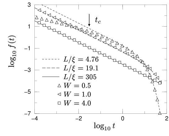
FIG. 1.: $\langle f(E,x;t)\rangle_{x}$ for a chain of length $L/a=2000$ with periodic boundary conditions, $E=0$ and $\eta=0.2$. The lines are determined from Eq. (3). The arrow indicates $t_{\rm c}$ for $L/\xi=4.76$.

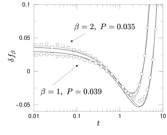
FIG. 2.: $\langle\delta f_{\beta}(E,x;t)\rangle_{x}$ for a $128\times 8\times 8$ lattice with $E=-1.7$, $\eta=0.01$, and $W=1.0$. For $\beta=1$ ($\circ$) and $\beta=2$ ($\Box$), these results are compared to Eqs. (4),(5) ( ) and Eq. (9) ( ).

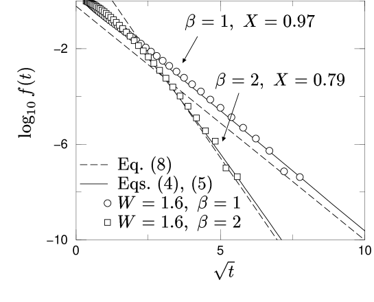
FIG. 3.: $f_{\beta}(E,x;t)$ for a $128\times 4\times 4$ lattice; for $X\stackrel{{\scriptstyle<}}{{\sim}}1$, $x\simeq L/2$, $W=1.6$, $E=-1.7$, $\eta=0.01$ and $\beta=1,2$ compared to Eqs. (4), (5) and (10).

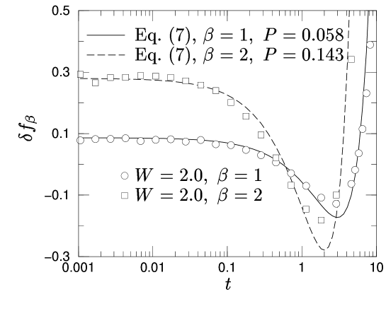
FIG. 4.: $\langle\delta f_{\beta}(E,{\mathchoice{{\hbox{\boldmath$\displaystyle r$}}}{{\hbox{\boldmath$\textstyle r$}}}{{\hbox{\boldmath$\scriptstyle r$}}}{{\hbox{\boldmath$\scriptscriptstyle r$}}}};t)\rangle_{{\mathchoice{{\hbox{\boldmath$\displaystyle r$}}}{{\hbox{\boldmath$\textstyle r$}}}{{\hbox{\boldmath$\scriptstyle r$}}}{{\hbox{\boldmath$\scriptscriptstyle r$}}}}}$ for a $100\times 100$ lattice with periodic BC, for $E=-1.6$ and $\eta=0.005$.

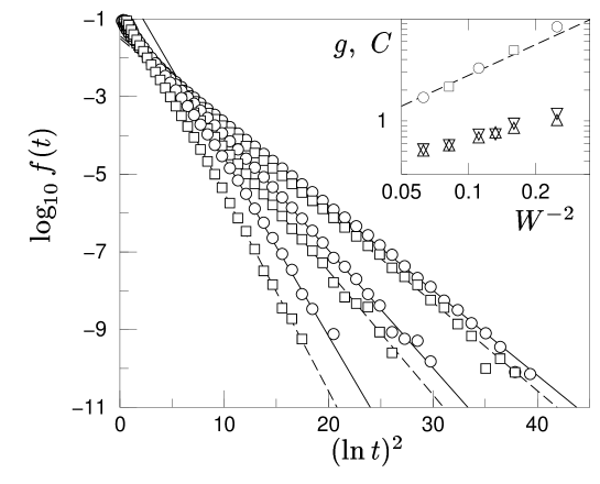
FIG. 5.: Tails of $\langle f_{\beta}(E,{\mathchoice{{\hbox{\boldmath$\displaystyle r$}}}{{\hbox{\boldmath$\textstyle r$}}}{{\hbox{\boldmath$\scriptstyle r$}}}{{\hbox{\boldmath$\scriptscriptstyle r$}}}};t)\rangle_{{\mathchoice{{\hbox{\boldmath$\displaystyle r$}}}{{\hbox{\boldmath$\textstyle r$}}}{{\hbox{\boldmath$\scriptstyle r$}}}{{\hbox{\boldmath$\scriptscriptstyle r$}}}}}$ for the same system as in Fig. 4, for $W=2,3$ and $4$, for $\beta=1$ ($\circ$) and $\beta=2$ ($\Box$). The lines show Eq. (11). The inset shows the fitted values of $C$ versus $W^{-2}$, for $\beta=1$ ($\bigtriangleup$) and $2$ ($\bigtriangledown$) and the dimensionless conductance $g$ for $\beta=1$ ($\circ$) and $2$ ($\Box$). The dashed line indicates $W^{-2}$ behaviour.

REFERENCES

[1] M. L. Mehta, Random Matrices and the Statistical Theory of Energy
Levels, Academic Press, New York, 1991.
[2] C. E. Porter, in: Statistical Theories of Spectra,
ed: C. E. Porter, Academic Press, New York, 1965, p. 1.
[3] M. Berry, in: Chaos and Quantum Physics,
eds.: M. J. Giannoni, A. Voros and J. Zinn–Justin,
North–Holland, Amsterdam, 1991, p. 201; M. Wilkinson,
J. Phys. A: Math. Gen. 21, 1173, (1988).
[4] F. Haake, Quantum Signatures of Chaos, Springer, Heidelberg, 1991.
[5] K. B. Efetov, Adv. Phys. 32, 53 (1983);
Supersymmetry in Disorder and Chaos,
Cambridge University Press, Cambridge, 1997.
[6] B.L. Altshuler, V. E. Kravtsov and I. V. Lerner, in:
Mesoscopic Phenomena in Solids, eds. B.L. Altshuler,
P. A. Lee and R. A. Webb, North-Holland, Amsterdam, 1991.
[8] A. D. Mirlin and Y. V. Fyodorov,
J. Phys. A: Math. Gen. 26, L551 (1993).
[9] Y. V. Fyodorov and A. Mirlin,
Int. J. Mod. Phys. B 8, 3795 (1994).
[10] V. I. Fal’ko and K. B. Efetov,
Europhys. Lett. 32, 627 (1995);
Phys. Rev. B 52, 17413 (1995).
[11] Y. V. Fyodorov and A. D. Mirlin,
Phys. Rev. B 51, 13403 (1995).
[12] A. D. Mirlin, J. Math. Phys. 38, 1888 (1997).
[13] A. D. Mirlin, Phys. Rep. 326, 259 (2000).
[14] B. Muzykantskii and D. E. Khmelnitskii,
JETP Lett. 62, 76 (1995).
[15] O. Agam, B. L. Altshuler and A. V. Andreev,
Phys. Rev. Lett. 75, 4389 (1995).
[16] E. Bogomolny and J. P. Keating, Phys. Rev. Lett.
77, 1472 (1996).
[17] R. Prange,
Phys. Rev. Lett. 77, 2447 (1996).
[18] B. Mehlig and M. Wilkinson, cond-mat/9905412.
[19] I. E. Smolyarenko and B. L. Altshuler,
Phys. Rev. B 55, 10451 (1997).
[20] J. Zittartz and J. S. Langer,
Phys. Rev.. 148, 741 (1966).
[21] A. Kudrolli, V. Kidambi and Sridhar,
Phys. Rev. Lett. 76, 822 (1995);
P. Pradhan and S. Sridhar, cond-mat/0003503 (2000).
[22] U. Kuhl, PhD dissertation, University of Marburg (1998);
U. Kuhl and H.-J. Stöckmann, Physica E, in press.
[23] P. W. Anderson, Phys. Rev. 109, 1492 (1958).
[24] E. Hofstetter and M. Schreiber,
Phys. Rev. B 48, 16979 (1993).
[25] K. Müller, B. Mehlig, F. Milde and M. Schreiber,
Phys. Rev. Lett. 78, 215 (1997).
[26] J. Cullum and R. A. Willoughby,
Lanczos Algorithms for Large Symmetric
Eigenvalue Computations, Birkhäuser, Boston, 1985.
[27] Here is defined so that a typical wavefunction
decays according to ) away
from the localization center .
With this choice of , one has
to second order in .
[28] K. B. Efetov and A. I. Larkin, Sov. Phys. JETP 58,
444 (1983).
[29] V. Uski, B. Mehlig, R.A. Römer, M. Schreiber,
Physica B, in press.
FIG. 1.:
for a chain of length with periodic boundary conditions,
and . The lines
are determined from Eq. (3).
The arrow indicates for .
FIG. 2.:
for a lattice
with , , and . For
() and (),
these results are compared to Eqs. (4),(5)
() and Eq. (9)
().
FIG. 3.:
for a
lattice; for ,
, , ,
and compared to Eqs. (4), (5)
and (10).
FIG. 4.:
for a
lattice with periodic BC,
for and .
FIG. 5.:
Tails of
for the same system as in Fig. 4,
for and , for
() and ().
The lines show Eq. (11). The inset shows the fitted values of
versus , for ()
and ()
and the dimensionless conductance for
() and ().
The dashed line indicates behaviour.