Abstract

We introduce a nonextensive entropic measure $S_{\chi}$ that grows like $N^{\chi}$, where $N$ is the size of the system under consideration. This kind of nonextensivity arises in a natural way in some $N$-body systems endowed with long-range interactions described by $r^{-\alpha}$ interparticle potentials. The power law (weakly nonextensive) behavior exhibited by $S_{\chi}$ is intermediate between (1) the linear (extensive) regime characterizing the standard Boltzmann-Gibbs entropy and the (2) the exponential law (strongly nonextensive) behavior associated with the Tsallis generalized $q$-entropies. The functional $S_{\chi}$ is parametrized by the real number $\chi\in[1,2]$ in such a way that the standard logarithmic entropy is recovered when $\chi=1$ . We study the mathematical properties of the new entropy, showing that the basic requirements for a well behaved entropy functional are verified, i.e., $S_{\chi}$ possesses the usual properties of positivity, equiprobability, concavity and irreversibility and verifies Khinchin axioms except the one related to additivity since $S_{\chi}$ is nonextensive. For $1<\chi<2$, the entropy $S_{\chi}$ becomes superadditive in the thermodynamic limit. The present formalism is illustrated by a numerical study of the thermodynamic scaling laws of a ferromagnetic Ising model with long-range interactions.

Keywords: entropy, nonextensivity, long-range interactions.

PACS: 05.20.-y;05.20.Gg;02.70.Lq;75.10.HK;05.70.Ce

1. Introduction

There is nowadays an intense research activity on the mathematical properties and physical applications of new versions of the Maximum Entropy Principle based on generalized or alternative entropic functionals [1, 2, 3, 4, 5, 6, 7, 8, 9, 10, 11, 12, 13, 14, 15, 16, 17, 18]. This line of inquiry has been greatly stimulated by the work of Tsallis, who showed that it is possible to build up a mathematically consistent and physically meaningful generalization of the standard Boltzmann-Gibbs-Jaynes thermostatistical formalism on the basis of a nonextensive entropic measure [1]. The main motivation behind Tsallis proposal is that there are important physical scenarios, such as self-gravitating systems [19, 20], electron-plasma two dimensional turbulence[21], among many others, which are characterized by a nonextensive behavior: due to the long range of the relevant interactions some of the thermodynamic variables usually regarded as additive, such as the internal energy, lose their extensive character. This suggests that a nonextensive (non-additive) entropy functional might be appropriate for their thermostatistical description. The Jaynes MaxEnt approach to Statistical Mechanics [22, 23] suggests in a natural way the possibility of incorporating alternative entropy functionals to the variational principle. The new entropy functional introduced by Tsallis has the form [1]

$$S_{q}=\frac{1}{q-1}\left(1-\sum_{i=1}^{w}p_{i}^{q}\ \right),$$ (1)

where $(p_{i},\,\,\,i=1,\ldots,w)$ are the microstate probabilities describing the system under consideration and the entropic index $q$ is any real number. The standard Boltzmann-Gibbs entropy $S=-\sum_{i=1}^{w}p_{i}\ln p_{i}$ is recovered in the limit $q\rightarrow 1$. The measure $S_{q}$ is nonextensive: The entropy of a composite system $A\oplus B$ constituted by two subsystems $A$ and $B$, independent in the sense that $p^{(A\oplus B)}_{ij}=p^{(A)}_{i}p^{(B)}_{j}$, verifies the Tsallis’ $q$-additive relation

$$S_{q}(A\oplus B)=S_{q}(A)+S_{q}(B)+(1-q)S_{q}(A)S_{q}(B).$$ (2)

We see from the above equation that the Tsallis’ parameter $q$ can be regarded as a measure of the degree of nonextensivity. Many relevant mathematical properties of the standard thermostatistics are verified by the Tsallis’ generalized formalism or can be appropriately generalized [1, 18]. Self-gravitating systems constituted the first physical problem discussed within Tsallis’ nonextensive thermostatistics [20] and Tsallis’ theory has recently been applied to other physical problems [24, 25, 26, 27, 28, 29]. One of the main consequences of the intensive effort devoted in recent years to the study of Tsallis theory is that there is now a growing consensus that there are many problems in statistical physics, biology, economics, and other areas, where a generalization of the standard approach based on Boltzmann-Gibbs-Jaynes extensive entropy might be useful. A comprehensive bibliography on the current research literature on Tsallis’ theory and the statistical physics of nonextensive systems can be found in [30, 31].

Inspired on Tsallis’ pioneering proposal, various nonextensive entropic measures endowed with interesting properties have been recently advanced [6, 7, 8, 9, 10, 11, 12]. Moreover, it has been proved that some physically relevant mathematical properties are shared by large families of entropic measures [3, 4]. The aim of the present work is to explore the possibility of developing a thermostatistical formalism based on a nonadditive entropic functional characterized by a degree of nonextensivity weaker than the one exhibited by Tsallis measure. As we shall see, Tsallis entropy varies exponentially with the size of the system under consideration. The new measure introduced here only scales as a power of the size of the system. That is to say, our proposal is tantamount of considering a nonextensive regime intermediate between (1) the standard extensive one associated with Boltzmann-Gibbs entropy, and (2) the exponentially nonextensive one described by Tsallis formalism.

There is an important physical motivation for introducing an entropy endowed with power law nonextensivity. Systems with long range interactions constitute the physical scenarios where the need of a generalization of the standard thermostatistical formalism can be more clearly appreciated. Consider a system of $N$ particles in a $d$-dimensional (one particle) configuration space. If the dependence of the interparticle potential with the interparticle distance $r$ is given by $r^{-\alpha}$, it can be shown that the system’s energy levels scale as [32]

$$N\tilde{N}\,=\,N\,\,\frac{N^{1-\alpha/d}\,-\,\alpha/d}{1\,-\,\alpha/d}.$$ (3)

Hence, for large $N$, the internal energy scales as a power of the size of the system. That is,

$$E\,\sim\,N^{2-\alpha/d}$$ (4)

In the case of extensive systems governed by short-range interactions, the internal energy $E$ and the the entropy $S$ scale in the same way: they both grow linearly with $N$. On the other hand, the temperature $T$ is an intensive variable and does not change with $N$. How can these scaling laws be generalized to the non-extensive setting? A possible path towards the alluded generalization starts with the Helmholtz free energy,

$$F\,=\,E\,-\,TS.$$ (5)

From the above expression it seems reasonable to expect both $E$ and $TS$ to scale in the same fashion [32]. The only way to fulfill this expectation, if the standard extensive entropy is used, is to require that the temperature scales as [32, 33]

$$T\,\sim\tilde{N}\,\sim\,N^{1-\alpha/d},$$ (6)

losing its intensive character.

It would be very appealing to have, within the nonextensive scenario, an entropy $S_{\chi}$ endowed with the same scaling law as the one exhibited by the energy. If, as it occurs for extensive systems, the entropy and the energy behave in the same way, the temperature would still be an intensive quantity. What we need in order to have a thermostatistical formalism with these nice properties is an entropy functional with power law nonextensivity, scaling as

$$S_{\chi}\,\sim\,N^{\chi}\,\sim\,N^{2-\alpha/d}.$$ (7)

From the above discussion it is clear that we are going to assume that the exponent $\chi$ appearing in the entropic scaling law is related with $d$ and $\alpha$ by

$$\chi\,=\,2\,-\,\alpha/d,$$ (8)

so that the physically motivated range of vales for $\chi$ is

$$1\,\leq\,\chi\,\leq 2.$$ (9)

The purpose of this work is to study the basic properties of a possible candidate for a weakly-nonextensive thermostatistics, and to consider its application to a magnetic system with long-range interactions. The paper is organized as follows. In Section II the exponential behavior of Tsallis entropy is analyzed and a power–law weakly nonextensive entropy is introduced. The basic mathematical properties of the new measure are studied in Section III. Two state systems are considered in Section IV. In Section V the weakly nonextensive entropy is applied to a ferromagnetic Ising model with long-range interactions. Finally, some conclusions are drawn in Section VI.

2. Exponential Vs. Power Law Nonextensivity

Tsallis Entropy and Exponential Nonextensivity

The nonextensive behavior of Tsallis functional, encapsulated in equation (2), is the most important single property distinguishing Tsallis measure from the standard additive logarithmic entropy. An important consequence of relation (2) that has not been fully appreciated in the literature is that Tsallis entropy may varies exponentially with the size of the system. In order to clarify the above assertion let us consider a system consisting of $N$ independent two-state subsystems. For simplicity we also assume that the system is described by an equiprobability distribution. That is, each of the $w=2^{N}$ possible microstate of the system has probability $1/w$. The associated Tsallis measure adopts then the value $S_{q}^{equiprob.}\,=\,\frac{1-w^{1-q}}{q-1}$, so that, for $q<1$ and large $N$,

$$S_{q}\,\sim\,\frac{1}{1-q}\,\,2^{(1-q)N}.$$ (10)

If $q>1$ the $q$-entropy tends to the constant limit value $\frac{1}{q-1}$ as $N\rightarrow\infty$. We are going to consider only the $q<1$ regime. In that case the $q$-entropy exhibits an exponential behavior as a function of the size $N$ of the system. In general, the entropy $S_{q}(N)$ of a composite system $A=\oplus_{j=1}^{N}A^{(j)}$ consisting on $N$ identical and independent subsystems $\{A^{(j)},\,\,j=1,\ldots N\}$, is given by

$$S_{q}(N)\,=\,\frac{1}{q-1}\,\left\{1\,-\,[1+(1-q)S_{q}(1)]^{N}\right\},$$ (11)

where $S_{q}(1)$ stands for the individual entropy of each constituent subsystem $A^{(j)}$. Notice that in order to obtain the above expression it is not necessary to assume that each subsystem $A^{(j)}$ is described by an equiprobability distribution.

Power Law Nonextensive Entropy

We believe that it is worth exploring the possibility of a thermostatistical formalism based on a nonextensive entropy $S_{\chi}$ growing as a power $N^{\chi}$ of the size of the system, instead of growing exponentially. In accord with the physical arguments discussed in the Introduction (see equations (8-9)), we shall restrict our considerations to values of $\chi\in[1,2]$ . Let us assume that the functional $S_{\chi}$ associated with a given discrete probability distribution $\{p_{i},\;i=1,\ldots,w\}$ is given by

$$S_{\chi}=\sum_{i=1}^{w}\phi_{\chi}(p_{i}),$$ (12)

$\phi_{\chi}(p_{i})$ being an appropriate function of the individual microstate probabilities $p_{i}$. In order to find a suitable expression for the function $\phi_{\chi}(z)$ it is enough to consider again the equiprobability distribution associated with a collection of $N$ identical independent two state subsystems. In that case we have $w=2^{N}$ and

$$S_{\chi}\, = \,w\,\phi_{\chi}(1/w)$$ (13)

$$= \,2^{N}\phi_{\chi}(2^{-N})$$ (14)

$$\sim N^{\chi},$$ (15)

which implies

$$\phi_{\chi}(2^{-N})\,\sim\,2^{-N}N^{\chi}.$$ (16)

The simplest choice for a function $\phi_{\chi}(z)$ complying with the above relation is

$$\phi_{\chi}(z)\,=\,z(-\ln z)^{\chi}.$$ (17)

Unfortunately, this function is not adequate for our purposes. Its second derivative $d^{2}\phi_{\chi}/dz^{2}$ lacks a definite sign within the relevant range of values of $z$ and $\chi$, leading thus to an entropy functional without a definite concavity. However, since we are only interested in the large $N$ asymptotic regime, any function $\phi_{\chi}(z)$ behaving like (17) in the limit $z\rightarrow 0$ would do. As we shall see, the function

$$\phi_{\chi}(z)\,=\,\frac{1}{2}\,\left[z(-\ln z)^{\chi}+z(-\ln z)^{1/\chi}\right]$$ (18)

leads to the measure

$$S_{\chi}\,=\,\frac{1}{2}\,\sum_{i=1}^{w}\,\left[p_{i}(-\ln p_{i})^{\chi}+p_{i}(-\ln p_{i})^{1/\chi}\right],$$ (19)

which complies with all the basic properties of a well behaved entropy. It is clear that in the case $\chi=1$ the standard entropy $S_{1}=-{\displaystyle\sum_{i=1}^{w}}p_{i}\ln{p_{i}}$ is recovered.

The optimization of $S_{\chi}$ under the constraints imposed by normalization,

$$\sum_{i=1}^{w}p_{i}\;=\;1,$$ (20)

and the mean values

$$\;\;\;\;\;\;\;\;\;\;\langle{\cal A}^{(r)}\rangle\;\equiv\;\sum_{i=1}^{w}p_{i}{\cal A}^{(r)}_{i}\;=\;{\cal A}_{\chi}^{(r)}\;\;\;\;\;\;\;\;\;(r=1,\ldots,R)$$ (21)

of a given set $\{{\cal A}^{(r)}\}$ of observable leads to the variational problem

$$\delta\left\{S_{\chi}\,-\,\sum_{r=1}^{R}\beta_{r}\langle{\cal A}^{(r)}\rangle\,-\,\alpha\,\sum_{i=1}^{w}p_{i}\right\}\,=\,0,$$ (22)

whose solution is of the form

$$p_{i}=F\left(\alpha+\sum_{r=1}^{R}\beta_{r}{\cal A}_{i}^{(r)}\right)\;\;\;\;\;\;\;i=1,\dots,w.$$ (23)

Here $\alpha$ and $\{\beta_{r}\}$ are appropriate Lagrange multipliers and $F(z)$ is the inverse function of

$$\phi_{\chi}^{\prime}(z)\,=\,\frac{1}{2}\left\{(-\ln z)^{\chi}+(-\ln z)^{\frac{1}{\chi}}-\chi(-\ln z)^{\chi-1}-\frac{1}{\chi}(-\ln z)^{\frac{1}{\chi}-1}\right\},$$ (24)

which verifies the relation

$$F[\phi_{\chi}^{\prime}(z)]\,=\,\phi_{\chi}^{\prime}[F(z)]\,=\,z.$$ (25)

The function $F(z)$ is well defined because the second derivative of $s_{\chi}(z)$ is negative,

$$\frac{{\rm d}^{2}s_{\chi}}{{\rm d}z^{2}}\; = \;\frac{1}{2z}\left[\chi(\chi-1)(-\ln z)^{\chi-2}\,+\frac{1}{\chi}\left(\frac{1}{\chi}-1\right)(-\ln z)^{\frac{1}{\chi}-2}\,\right.$$ (27)

$$\,-\left.\chi(-\ln z)^{\chi-1}\,+\frac{1}{\chi}(-\ln z)^{\frac{1}{\chi}-1}\right]$$

$$< 0,$$ (28)

for $0<z<1$, and $1<\chi<2$. Actually, $s^{\prime\prime}_{\chi}(z)$ has a definite (negative) sign within the larger interval $[1/\chi_{c},\chi_{c}]$, where $\chi_{c}\approx 2.1762$. This can be appreciated in Fig. 1, where the real roots of $s^{\prime\prime}_{\chi}(z)=0$ are depicted as a function of $\chi$. We see that there are no real roots $\chi\in[1/\chi_{c},\chi_{c}]$.

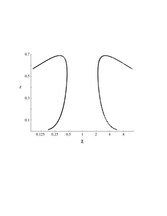
FIG. 1.: The real roots of $s^{\prime\prime}_{\chi}(z)=0$ as a function of $\chi$. There are no real roots within the interval $[1/\chi_{c},\chi_{c}]$, where $\chi_{c}\approx 2.1762$.

It is important to realize that the lack of a simple analytical expression for the function $F(z)$ does not constitute a serious conceptual problem, nor does it pose any practical difficulty for the numerical treatment of problems involving the MaxEnt distributions (23). The form of the function $F(z)$ is shown in Fig. 2.

FIG. 2.: The function $F(z)$ defined by the equations (24-25) for $\chi=1.0,1.25,1.5,1.75,2.0$.

The canonical ensemble probability distribution associated with the entropy $S_{\chi}$,

$$p_{i}\,=\,F(\alpha\,+\,\beta\epsilon_{i}),$$ (29)

is obtained when the $S_{\chi}$ is extremalized under the constraints of normalization and the mean value of the energy,

$$\langle U\rangle\,=\,\sum_{i}p_{i}\epsilon_{i},$$ (30)

where $\epsilon_{i}$ stands for the energy of the microstate $i$. The Lagrange multiplier $\beta$ appearing in (29) is the one associated with the energy constraint and corresponds, within the present thermostatistical formalism, to the inverse temperature. That is, taking Boltzmann constant $k=1$, we have $\beta=1/T$.

3. Main Properties of the New Entropy

3.1 Khinchin axioms

Khinchin proposed a set of four axioms[34], which are usually regarded as reasonable requirements for a well behaved information measure. Our entropy measure $S_{\chi}$ verifies the first three of them:
(i) $\;\;\;\;\;S_{\chi}=S_{\chi}(p_{1},\ldots,p_{w})$,
i.e., the entropy is a function of the probabilities $p_{i}$ only.
(ii) $\;\;\;\;S_{\chi}(p_{1},\ldots,p_{w})\;\leq\;S_{\chi}(\frac{1}{w},\ldots,\frac{1}{w})\;\equiv\;S_{\chi}^{equipr.}(w)$,
i.e., $S_{\chi}$ adopts its extreme at equiprobability (this property will be proved in subsection 3.2).
(iii) $\;\;\;S_{\chi}(p_{1},\ldots,p_{w})\;=\;S_{\chi}(p_{1},\ldots,p_{w},0)$,
this property, known as expansibility, is clearly verified since $\phi_{\chi}(0)=0$.
(iv)   The fourth Khinchin axiom concerns the behavior of the entropy of a composite system in connection to the entropies of the subsystems. We will comment on this axiom later.

3.2 General mathematical properties

Let us now consider the properties related to positivity, certainty, concavity, equiprobability, additivity and irreversibility, which are some of the most important features characterizing an information or entropic measure [1, 8, 12, 13].

3.2.1 Positivity

It is plain from equation (18) that $\phi_{\chi}(0)=\phi_{\chi}(1)=0$ and also that $\phi_{\chi}(p)\geq 0$ for $p\in[0,1]$. This implies the positivity condition

$$S_{\chi}\geq 0.$$ (31)

3.2.2 Certainty

The equality symbol in Eq. (31) holds only at certainty, i.e.,

$$S_{\chi}(1,0,\ldots,0)\;=\;0.$$ (32)

Indeed, $S_{\chi}$ vanishes if and only if we have certainty.

3.2.3 Concavity

Considering $(p_{1},\ldots,p_{w})$ as independent variables, the second partial derivatives of $S_{\chi}$ are

$$\frac{\partial^{2}S_{\chi}}{\partial p_{j}\partial p_{k}}\;=\;\frac{\partial^{2}S_{\chi}}{\partial^{2}p_{j}}\,\delta_{jk}\;<0\;\;\;\;\;\;\;\;\;\mbox{for}\;\;\;0<p_{j}<1.$$ (33)

Expression (33) guarantees definite concavity over probability space (see, for instance, [23]).

3.2.4 Equiprobability

The probability distribution that extremizes $S_{\chi}$ under the normalization constraint is

$$p_{i}\,=\,F(\alpha)\,=\,1/w$$ (34)

Therefore, since $S_{\chi}$ has negative concavity, it is maximal at equiprobability. A well behaved entropy should also be, at equiprobability, a monotonically increasing function of the number of states $w$. For large $w$ we have $S_{\chi}(w)\sim(\ln w)^{\chi}$. Therefore, for large values of $w$, $S_{\chi}^{equipr.}(w)$ is an increasing function of $w$.

3.2.5 Nonextensivity

The nonextensive behavior of the entropy $S\chi$ is determined by the relation of the entropy of a composite system with the individual entropies of its constituent subsystems. Let us consider systems $A$ and $B$ with associated probabilities $\{a_{i},\;i=1,\ldots,w_{A}\}$ and $\{b_{j},\;j=1,\ldots,w_{B}\}$, respectively. If systems $A$ and $B$ are independent, i.e., the composite system $A\oplus B$ has associated probabilities $\{a_{i}b_{j};\;i=1,\ldots,w_{A};\;j=1,\ldots,w_{B}\}$, then the entropy $S_{\chi}(A\oplus B)$ of the composite system minus the sum of the entropies of its subsystems,

$$\Delta S_{\chi}(A,B)\,\equiv\,S_{\chi}(A\oplus B)-S_{\chi}(A)-S_{\chi}(B)$$ (35)

is the quantity characterizing the nonextensive features of the measure $S_{\chi}$. When $\Delta S_{\chi}(A,B)>0$($\Delta S_{\chi}(A,B)<0$) we have superaditivity (subadditivity). From the examination of particular examples we conclude that $\Delta S_{\chi}(A,B)$ does not have always the same sign. However, the region of probability space where $\Delta S_{\chi}(A,B)$ is positive is much larger than the region where that quantity is negative. Furthermore, if we consider $N$ identical subsystems (instead of just two of them), the region of probability space corresponding to subadditive behavior tends to vanish as $N$ grows. consequently, the entropy $S_{\chi}$ becomes superextensive in the thermodynamic limit. Particular examples illustrating these features of the measure $S_{\chi}$ are provided in Section IV. Moreover, in Section V we are going to consider the nonextensivity of $S_{\chi}$ in connection with the thermodynamic properties of an Ising model endowed with long–range interactions.

3.2.6 Irreversibility

One of the most important roles played by entropic functionals within theoretical physics is to characterize the “arrow of time”. When they verify an $H$-theorem, they provide a quantitative measure of macroscopic irreversibility. We will now show, for some simple systems, that the present measure $S_{\chi}$ satisfies an $H$-theorem, i.e., its time derivative has a definite sign.

Let us calculate the time derivative of $S_{\chi}$

$$\frac{{\rm d}S_{\chi}}{{\rm d}t}\;=\;\sum_{i=1}^{w}\,\frac{{\rm d}p_{i}}{{\rm d}t}s^{\prime}_{\chi}(p_{i}),$$ (36)

for a system whose probabilities $p_{i}$ evolve according to the master equation

$$\frac{{\rm d}p_{i}}{{\rm d}t}\;=\;\sum_{j=1}^{w}[P_{ji}p_{j}-P_{ij}p_{i}],$$ (37)

where $P_{ij}$ is the transition probability per unit time between microscopic configurations $i$ and $j$. Assuming a system with a uniform equilibrium distribution and detailed balance, i.e., $P_{ij}=P_{ji}$, we obtain from (36)

$$\frac{{\rm d}S_{\chi}}{{\rm d}t}\;=\;\frac{1}{2}\sum_{i=1}^{w}\sum_{j=1}^{w}\,P_{ij}\,(p_{i}-p_{j})\biggl{(}s^{\prime}_{\chi}(p_{j})\,-\,s^{\prime}_{\chi}(p_{i})\biggr{)}.$$ (38)

Since $s_{\chi}^{\prime\prime}(p_{i})<0$, the quantities $(p_{i}-p_{j})$ and $(s^{\prime}_{\chi}(p_{j})\,-\,s^{\prime}_{\chi}(p_{i}))$ have the same sign. Then we obtain

$$\frac{{\rm d}S_{\chi}}{{\rm d}t}\;\geq\;0.$$ (39)

The equality holds for equiprobability, i.e., at equilibrium, while in any other cases the entropy $S_{\chi}$ increases with time. Therefore, $S_{\chi}$ exhibits irreversibility.

3.2.7 Jaynes thermodynamic relations

It is noteworthy that, within the present MaxEnt formalism, the usual thermodynamical relations involving the entropy, the relevant mean values, and the associated Lagrange multipliers, i.e.,

$$\frac{\partial S_{\chi}}{\partial\langle{\cal A}^{(r)}\rangle}\;=\;\beta_{r}$$ (40)

are verified. Hence, our formalism exhibits the usual thermodynamical Legendre transform structure. Actually, this property is verified by a wide family of entropy functionals[3, 4]. A particular important example of (40) is furnished by the canonical ensemble thermodynamic relation

$$\frac{\partial S_{\chi}}{\partial\langle U\rangle}\;=\;\beta\;=\;\frac{1}{T}.$$ (41)

4. Two-state systems

In order to illustrate some of the above properties, we consider a two-state system (with associated probabilities $\{p,1-p\}$). In this case, $S_{\chi}$ only depends on the variable $p$. In fact, from its definition, we have

$$S_{\chi}(p)\,=\,\frac{1}{2} \left[p(-\ln p)^{\chi}+p(-\ln p)^{\frac{1}{\chi}}\right.$$ (43)

$$+\,\left.(1-p)(-\ln(1-p))^{\chi}+(1-p)(-\ln(1-p))^{\frac{1}{\chi}}\right],$$

FIG. 3.: Entropy $S_{\chi}$ for a two-state system ($w=2$) as a function of $p$ for different values of $\chi$ indicated on the figure.

The shape of $S_{\chi}(p)$ for different values of $\chi$ is shown in Fig. 3, which exhibits the positivity and concavity of $S_{\chi}$. In fact, from expression (43), the first derivative of $S_{\chi}(p)$ vanishes at $p=1/2$ and ${\rm d}^{2}S_{\chi}/{\rm d}p^{2}<0\;\;\forall p\in[0,1]$. Since the second derivative is always negative, $S_{\chi}(p)$ is maximal at equiprobability. Moreover, as shown in the general case, taking into account the concavity of $S_{\chi}$ and that $S_{\chi}$ vanishes at the certainty, then $S_{\chi}$ is positive for all $p$.

The non-additivity of $S_{\chi}$ is illustrated in Fig. 4 for two independent two-state systems $A$ (with probabilities $p$ and $1-p$) and $B$ (with probabilities $q$ and $1-q$), through the plot of the relative difference

$$(\Delta S_{\chi})_{rel.}=[S_{\chi}(A\oplus B)-(S_{\chi}(A)+S_{\chi}(B))]/S_{\chi}(A\oplus B)$$ (44)

as a function of $p$ and $q$. For most values of $p$ and $q$ the nonextensive measure $S_{\chi}$ behaves in a superadditive fashion. Only for values lying in a small region near the edges of the $(p,q)-$square does $S_{\chi}$ become subextensive.

                                                    

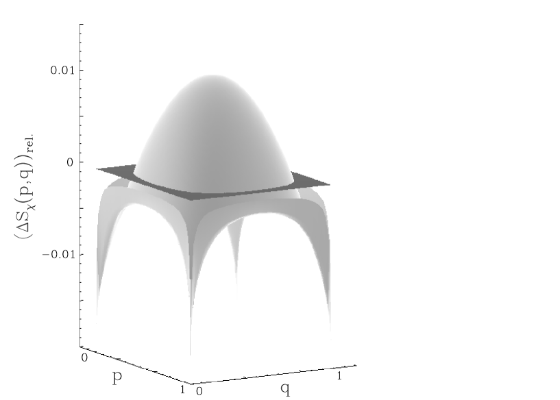
FIG. 4.: The subadditivity and superaditivity of $S_{\chi}$. The quantity $(\Delta S_{\chi})_{rel.}$ as a function of $p$ and $q$, for a composite system constituted by the independent two-state subsystems $A$ (with associated probabilities $\{q,1-q\}$), and $B$ (with associated probabilities $\{p,1-p\}$).

The nonextensive behavior of $S_{\chi}$ in the thermodynamic limit can be illustrate by recourse to a system constituted by $N$ two-state subsystem. Let us first assume that each one of the subsystems is described by the same probabilities $p$ and $(1-p)$. Consequently, the entropy associated with the composite system is

$$S_{\chi}(N)=\frac{1}{2^{N}}\sum_{k=0}^{N}\left(\begin{array}[]{c}N\\ k\end{array}\right)p^{k}(1-p)^{N-k}\left[\left(-\ln(p^{k}\,(1-p)^{N-k}\right)^{\chi}+\left(-\ln(p^{k}\,(1-p)^{N-k}\right)^{\frac{1}{\chi}}\right]$$ (45)

It can be shown after some algebra that, for $0<p<1$,

$$[-\ln(1-p)]^{\chi}N^{\chi}\,<\,S_{\chi}(N)\,<\,[-\ln p]^{\chi}N^{\chi}+[-\ln p]^{1/\chi}N^{1/\chi}.$$ (46)

Hence, for any given value of $p\in(0,1/2)$ there exist an $M$ such that

$$N>M\,\Longrightarrow\,S_{\chi}(N)>NS_{\chi}(1),$$ (47)

which means that $S\chi$ becomes superadditive for large enough values of $N$. This is shown in Fig. 5a , where the quantity

$$(\Delta S_{\chi})_{rel.}\,=\,[S_{\chi}(N)\,-\,NS_{\chi}(1)]/S_{\chi}(N)$$ (48)

is depicted for different values of $N$. In a similar way, Fig. 5b shows the behavior of $(\Delta S_{\chi})_{rel.}$ as a function of $p$ for a composite system consisting of $N-1$ two-state subsystems each with probabilities $\{\frac{1}{2},\frac{1}{2}\}$ along with one extra subsystem with probabilities $p$ and $(1-p)$.

FIG. 5.: The superaditivity of $S_{\chi}$ in the thermodynamic limit. (a) The quantity $(\Delta S_{\chi})_{rel.}$ associated with a system constituted by $N$ identical two-state subsystems with probabilities $p$ and $(1-p)$, as a function of $p$ and for different values of $N$. (b) $(\Delta S_{\chi})_{rel.}$ as a function of $p$ for a system constituted by $N-1$ identical two-state subsystems with probabilities $\{\frac{1}{2},\frac{1}{2}\}$ along with one extra two-state subsystem with probabilities $p$ and $(1-p)$.

5. Ferromagnetic Ising Model with Long-Range Interactions

In this section we apply the canonical thermostatistics associated with the entropy $S_{\chi}$ to an $N$-body system described by an $r^{-\alpha}$ interparticle potential. The energy of this kind of systems scales as a power of the number of particles [32]. The consideration of systems exhibiting this power-law nonextensivity constituted our main motivation for introducing the measure $S_{\chi}$. As argued in Section I, an entropy endowed with the same non-extensive behavior as the one associated with the energy may lead to a thermostatistical description preserving the intensive character of the temperature. In order to illustrate these ideas we are going to study a long-range Ising model described by the Hamiltonian

$${\cal H}\,=\,J\,\sum_{i,j=1}^{N}\,\frac{1\,-\,S_{i}S_{j}}{r^{\alpha}_{ij}},\,\,\,\,\,\,\,\,\,\,\,(S_{i}=\pm 1,\forall i),$$ (49)

where $J$ is an appropriate coupling constant, and the sum runs over all the pairs of sites on a $d$-dimensional lattice with periodic boundary conditions and $r_{ij}$ stands for the distance between the sites $i$ and $j$. It is clear that the range of the interaction is determined by the value of the exponent $\alpha$. In particular, the standard (short-range) first-neighbors interaction is recovered in the limit $\alpha\rightarrow\infty$, while the mean field approximation is obtained when $\alpha=0$ (replacing $J$ by $J/N$). These extreme cases illustrate, respectively, the two possible thermodynamic behaviors that, according to the value of $\alpha$, are admitted by the system (49). On the one hand we have the extensive regime corresponding to $\alpha>d$. On the other hand we have the non-extensive regime associated with $\alpha<d$. In order to clarify this let us estimate the internal energy per particle at zero temperature. We have [32]

$$\frac{E}{N}\,\sim\,\int_{1}^{\infty}drr^{d-1}r^{-\alpha}.$$ (50)

It is easy to see that the above integral converges if $\alpha>d$ and diverges if $0\leq\alpha\leq d$. The following is a standard notation used in previous works:

$$\tilde{N}\equiv 1+\frac{1}{d}\int_{1}^{N^{1/d}}drr^{d-1}r^{-\alpha}=\frac{N^{1-\alpha/d}-\alpha/d}{1-\alpha/d},$$ (51)

Here we consider the non–extensive regime for the one–dimensional case $d=1$ and $\alpha=0.8$. We have performed numerical simulations by using a novel approach recently introduced [2] to study systems with long range interactions governed by generalized entropies as the one considered here. The method relies upon the calculation of the number of states, $\Omega(\epsilon_{k})$, with a given energy $\epsilon_{k}$.

Note that, the number of possible configurations and associated probabilities $p_{i}$ is in general very large, $W=2^{N}$ for Ising models for example. However the number of permitted energies or energy levels $K$ is not so large, because there is a large number of states $\Omega(\epsilon_{k})$ sharing the same energy $\epsilon_{k}$. We can rewrite the sums in Eqs. (19,30) taking into account the $K$ energy levels weighted by $\Omega(\epsilon_{k})$:

$$S_{\chi} = \frac{1}{2}\sum_{k=1}^{K}\Omega(\epsilon_{k})p(\epsilon_{k})[(-\ln(p(\epsilon_{k}))^{\chi}+(-\ln(p(\epsilon_{k}))^{1/\chi}],$$ (52)

$$<O> = \sum_{k=1}^{K}\Omega(\epsilon_{k})p(\epsilon_{k})O(\epsilon_{k}).$$ (53)

Hence, the knowledge of the number of states $\Omega(\epsilon_{k})$ allows, by the use of these expressions, the calculation of the entropy and any averages of interest.

To calculate the probabilities $p(\epsilon_{k})$ we use the definition $p(\epsilon_{k})=F(\alpha+\beta\epsilon_{k})$, where the function $F$ is compute numerically as the inverse function of $s_{\chi}^{\prime}(z)$ (See Fig. 2).

To compute the histogram $\Omega(\epsilon_{k})$, the “Histogram by Overlapping Windows (HOW)” method [35, 2, 36] is used. A naive way of computing the histogram consists in generating different system configurations randomly and counting how many times a configuration with energy $\epsilon_{k}$ appears. However, since the $\Omega(\epsilon_{k})$ values span too many orders of magnitude it is not possible to find in this way a histogram over all the energy levels. The HOW method avoids this problem by generating system configurations only in a restricted energy interval and estimating the relative weights $\Omega(\epsilon_{k})/\Omega(\epsilon_{l})$ of these energy levels from the number of times they appear in the sample. From the overlap between energy intervals, one gets the complete $\Omega(\epsilon_{k})$ function, apart from an irrelevant normalization factor. Details about the HOW method can be found in [35, 36].

Finally we note a particularity of this new formalism, which is that the determination of the $\alpha$ constant from the normalization condition $\sum_{i}^{w}p_{i}=1$, require to solve the following equation

$$\sum_{k=1}^{K}\Omega(\epsilon_{k})F(\alpha+\beta\epsilon_{k})=1,$$ (54)

where $\epsilon_{k}$,$\beta$,$\Omega(\epsilon_{k})$ are input data for the equation. This equation for $\alpha$ was solved numerically using a dicotomic searching method.

Using the described procedure we have calculated the dependence over the temperature $T$ of the internal energy $E(N,T)$, spontaneous magnetization $M(N,T)=\mid\sum_{i=1}^{N}s_{i}\mid$, entropy $S(N,T)$ and free energy $F(N,T)=E-TS$ for the $1$–dimensional long–range Ising model in the non–extensive regime $\alpha=0.8$ and the corresponding value $\chi=1.2$ in the Eq. (8).

This system has been recently studied within the standard Boltzmann–Gibbs thermostatistics [33], as well as within Tsallis non–extensive $q$–formalism [2]. In [33] it was numerically verified that the scaling laws of the main thermodynamical quantities associated with the Gibbs canonical ensemble are

$$E(N,T)/(N\tilde{N})\, = \,e(T/\tilde{N}),$$ (55)

$$M(N,T)/N\, = \,m(T/\tilde{N}),$$ (56)

$$S(N,T)/N\, = \,s(T/\tilde{N}),$$ (57)

$$F(N,T)/(N\tilde{N})\, = \,f(T/\tilde{N}),$$ (58)

Since the energy and the entropy scale in different ways, the temperature $T$ has to be scaled as $T/\tilde{N}$. A similar situation arises within Tsallis $q$-generalized formalism, the concomitant scaling laws being [2]

$$E_{q}(N,T)/(N\tilde{N})\, = \,e(TA^{E}_{q}(N)/(N\tilde{N})),$$ (59)

$$M_{q}(N,T)/N\, = \,m(TA^{E}_{q}(N)/(N\tilde{N})),$$ (60)

$$S_{q}(N,T)/(A_{q}(N))\, = \,s(TA^{S}_{q}(N)/(N\tilde{N})),$$ (61)

$$F_{q}(N,T)/(N\tilde{N})\, = \,f(TA_{q}(N)/(N\tilde{N})),$$ (62)

where [2]

$$A_{q}(N)\, = \,(2^{N(1-q)}-1)/(1-q),$$ (63)

$$A^{S}_{q}(N)\, = \,(2^{N|1-q|}-1)/|1-q|,$$ (64)

$$A^{E}_{q}(N)\, = \,A_{q}(N)^{2}/A^{S}_{q}(N).$$ (65)

The scaling laws corresponding to the generalized $\chi$-canonical ensemble associated to the weakly nonextensive entropy $S_{\chi}$ are,

$$E(N,T)/(N\tilde{N})\, = \,e(TR_{\chi}(N)),$$ (66)

$$M(N,T)/N\, = \,m(TR_{\chi}(N)),$$ (67)

$$S_{\chi}(N,T)/(N^{\chi}+N^{1/\chi})\, = \,s(TR_{\chi}(N)),$$ (68)

$$F(N,T)/(N\tilde{N})\, = \,f(TR_{\chi}(N)),$$ (69)

where

$$R_{\chi}(N)\,=\,\frac{N^{\chi}\,+\,N^{1/\chi}}{N^{\chi}-(2-\chi)N}.$$ (70)

It is plain from the above equation that

$$\lim_{N\rightarrow\infty}R_{\chi}(N)\,=\,1,$$ (71)

so that for large enough values of $N$ the scaling laws (66) become

$$E(N,T)/(N^{\chi})\, = \,e(T),$$ (72)

$$M(N,T)/N\, = \,m(T),$$ (73)

$$S(N,T)_{\chi}/(N^{\chi})\, = \,s(T),$$ (74)

$$F(N,T)/(N^{\chi})\, = \,f(T).$$ (75)

According to the above equations, the thermodynamic curves of the Ising models (49) computed with increasing $N$-values must collapse without the need of a temperature rescalation. Numerical evidence of this scaling behavior is provided by Figures (6,7). It must be realized, however, that the $N$-values used are not large enough to see a complete collapse of the curves depicted. In order to reach complete collapse we need $R_{\chi}(N)\approx 1$ (see the insert of Figure (6b)).

FIG. 6.: Plot of (a) the internal energy and (b) the magnetization as a function of the scaled temperature. In the insert of (b) we plot with solid line the behavior of the scaling factor $R_{\chi}(N)$ for all the $N$ values and by points for the actual simulated sizes $N=100,400,1000,2000,3000$. We use here $\chi=1.2$.

We plot in Fig. 6 the scaled curves for the internal energy and magnetization using the Eqs. (66). In the insert of that plot we see the asimptotical behavior for the scaling factor $R_{\chi}(N)$, and with points we indicate the sizes plotted $N=100,400,1000,2000,3000$. Unfortunately we would need very large sizes $N\sim 10^{8}$ to observe an actual scaling without any scale factor, that is $R_{\chi}\sim 1$. However from the Fig.6 one can see that there is an actual tendency to the collapse. In fact we expect that the final universal curves will resemble to those corresponding to $N=2000,3000$ and we see in the Fig. 6 a tendency towards a complete collapse.

FIG. 7.: Plot of the entropy $S_{\chi}$ as a function of the scaled temperature for the indicated system sizes. In the insert we plot the expected no scale temperature behavior.

Also in Fig.7 we show the collapse for the entropy in the main plot with the scaled relations Eqs. (66) and in the insert without scaling. In addition we can see in this plot the actual superadditive behavior of the new entropy in an interacting system instead of the simple $N$ independent two states systems of the last section.

6. Conclusions

We have shown that the entropy functional $S_{\chi}$ verifies the main properties usually regarded as essential requirements for physically meaningful entropy functionals [1, 8, 12, 13]. The entropy $S_{\chi}$ verifies the first three Khinchin axioms. The measure $S_{\chi}$ satisfies the requirements of positivity, equiprobability, concavity and irreversibility. The associated MaxEnt scheme also complies with Jaynes thermodynamic relations. The properties verified by $S_{\chi}$ suggest that it might be a useful measure for describing nonextensive physical phenomena as well as for other practical applications.

The entropic functional $S_{\chi}$ grows as a power $N^{\chi}$ of the size $N$ of the system and is thus characterized by a weak nonextensive behavior (as opposed to the strong, exponential nonextensivity exhibited by Tsallis measure). An attentive reader might think that a power law nonextensive measure can be obtained in a trivial way by just defining a new ”entropy” equal to $(S_{Boltzmann})^{\chi}$. However, this simple proposal would not lead to anything new. The probability distributions maximizing $(S_{Boltzmann})^{\chi}$ are the same exponential distributions that maximize $S_{Boltzmann}$. This means that the standard (extensive) thermostatistics would be obtained again. On the contrary, the entropic functional $S_{\chi}$ furnishes a nontrivial new thermostatistics that might be appropriate for dealing with some nonextensive systems. As an application of the thermostatistical formalism associated with $S_{\chi}$ we considered a ferromagnetic Ising model with long-range interactions. We studied numerically the concomitant scaling laws.

Tsallis thermostatistics, which have attracted a great deal of attention recently [24, 25, 26, 27, 28, 29, 30, 31], arise from a nonextensive entropic measure $S_{q}$ growing exponentially with the size of the system. Now, if there are in Nature extensive systems (that is, those successfully studied within standard statistical mechanics and described by Gibbs exponential distributions) as well as Tsallis’ strong (exponentially) nonextensive systems, it is not unreasonable to expect also the existence of systems exhibiting an intermediate (weak) power-law kind of nonextensivity.

Let us consider a family of dynamical systems characterized by a set of parameters $\lambda$. We assume that there is a certain region $\Sigma$ in $\lambda$-space such that the system’s thermodynamic behavior is extensive for $\lambda\in\Sigma$ and nonextensive otherwise. It would be very surprising if, as a continuous change in the parameters $\lambda$ is considered, the system abruptly jumps from an extensive regime to an exponentially nonextensive one. It would be physically more sensible if there is an ”onset of nonextensivity” boundary between the extensive and nonextensive regions in $\lambda$-space, characterized by a weak, power-law nonextensive regime. A suggestive analogy can be made here with the onset of chaos is nonlinear dynamics. Consider, for instance, the well known Logistic map. For values of the map’s parameter corresponding to chaotic behavior the concomitant Lyapunov exponent is positive and near trajectories diverge exponentially in time. However, critical values of the map parameter associated with a vanishing Lyapunov exponent still do exhibit a form of ”weak chaos”. In those critical situations, corresponding to the onset chaos, near trajectories do not diverge exponentially in time: They diverge in a power-law way [37, 38].

It would be important to gain a further clarification of the physical meaning of the parameter $\chi$, and to understand under what circumstances might Nature choose to maximize the functional $S_{\chi}$. The only way to attain such an understanding is by a detailed study of the dynamics of particular nonextensive systems endowed with long range interactions . We hope that our present contribution may stimulate further work within this line of inquiry.

Acknowledgements

A.R.P. acknowledges the AECI Scientific Cooperation Program (Spain), and the CONICET (Argentine Agency) for partial financial support. R. Toral and R. Salazar acknowledges the financial support from DGES, grants PB94-1167 and PB97-0141-C02-01.

REFERENCES

REFERENCES

- [1] C. Tsallis, J. Stat. Phys. 52 (1988) 479; C. Tsallis, R.S. Mendes, and A.R. Plastino, Physica A 261 (1998) 534; E.M.F. Curado and C. Tsallis, J. Phys. A 24 (1991) L69.
- [2] R. Salazar and R. Toral, Phys. Rev. Lett. 83 (1999) 4233.
- [3] A. Plastino and A.R. Plastino, Phys. Lett. A 226 (1997), 257
- [4] R. S. Mendes, Physica A 242 (1997), 299; E.M.F. Curado, Braz. J. Phys. 29 (1999) 36.
- [5] P.T. Landsberg, Braz. J. Phys. 29 (1999) 46.
- [6] P.T. Landsberg and V. Vedral, Phys. Lett. A 247 (1998) 211.
- [7] S. Abe, Phys. Lett. A 224, 326 (1997).
- [8] A.R.R. Papa J. Phys. A 31, 1 (1998).
- [9] E.P. Borges and I. Roditi, Phys. Lett. A 246, 399 (1998).
- [10] C. Anteneodo and A.R. Plastino, J. Phys. A 32, 1089 (1999).
- [11] A.K. Rajagopal and S. Abe, Phys. Rev. Lett. 83 (1999) 1711.
- [12] R. Rossignoli and N. Canosa Phys. Lett. A 264 (1999) 148.
- [13] K.S. Fa, J. Phys. A 31, 8159 (1998).
- [14] D. Holste, I. Grosse, and H. Herzel, J. Phys. A 31, 2551 (1998).
- [15] E.P. Borges, J. Phys. A 31, 5281 (1998); E.K. Lenzi, E.P. Borges, and R.S. Mendes, J. Phys. A 32, 8551 (1999).
- [16] A. Compte and D. Jou, J. Phys. A 29 (1996) 4321; A. Compte, D. Jou, and Y. Katayama, J. Phys. A 30 (1997) 1023.
- [17] L. Borland, Phys. Rev. E 57 (1998) 6634.
- [18] E.K. Lenzi, L.C. Malacarne and R.S. Mendes, Phys. Rev. Lett. 80 (1998) 218.
- [19] W.C. Saslaw, Gravitational Physics of Stellar and Galactic Systems, Cambridge University Press, Cambridge, 1985.
- [20] A. R. Plastino and A. Plastino, Phys. Lett. A 174 (1993) 384.
- [21] B.M.R. Boghosian, Phys. Rev. E 53 (1995) 4754.
- [22] E.T. Jaynes, in Statistical Physics, ed. W.K. Ford (Benjamin, New York, 1963); A. Katz, Statistical Mechanics, (Freeman, San Francisco, 1967).
- [23] C. Beck and F. Schlögl, Thermodynamics of Chaotic Systems: An Introduction (Cambridge University Press, Cambridge, 1993).
- [24] C. Tsallis, S.V.F. Levy, A.M.C. Souza and R. Maynard, Phys. Rev. Lett. 75 (1995) 3589; Erratum: 77 (1996) 5442.
- [25] M. L. Lyra and C. Tsallis, Phys. Rev. Lett. 80 (1998) 53; C. Anteneodo and C. Tsallis, Phys. Rev. Lett. 80 (1998) 5313.
- [26] M. Buiatti, P. Grigolini, and A. Montagnini, Phys. Rev. Lett. 82 (1999) 3383.
- [27] A.K. Rajagopal, R.S. Mendes, and E.K. Lenzi, Phys. Rev. Lett. 80 (1998) 3907.
- [28] D.B. Ion and M.L.D. Ion, Phys. Rev. Lett. 81 (1998) 5714.
- [29] M.L.D. Ion and D.B. Ion, Phys. Rev. Lett. 83 (1999) 463.
- [30] C. Tsallis, Physics World 10, 42 (July 97); an updated bibliography on Tsallis’ theory an its applications is available at http://tsallis.cat.cbpf.br/biblio.htm
- [31] Several review articles on Tsallis’ thermostatistics and its applications appeared in Braz. J. Phys. 29 (1999), Special Issue, Nonextensive Statistical Mechanics and Thermodynamics, eds. S.R.A. Salinas and C. Tsallis, which can be seen at http://sbf.if.usp.br/WWW_pages/Journals/BJP/Vol29/Num1/index.htm
- [32] C. Tsallis, Fractals 3, 541 (1995).
- [33] S.A. Cannas and F.A. Tamarit, Phys. Rev. B54, R12661 (1996).
- [34] A.I. Khinchin, Mathematical Foundations of Information Theory (Dover, New York, 1957).
- [35] G. Bhanot, R. Salvador, S. Black, P. Carter, and R. Toral. Phys. Rev. Lett., 59 (1987) 803.
- [36] R. Salazar, and R. Toral. Thermostatistics of extensive and Nonextensive Systems Using Generalized Entropies, (2000), preprint.
- [37] C. Tsallis, A.R. Plastino, and W.-M. Zheng. Chaos, Solitons and Fractals, 8 (1997) 885.
- [38] U.M.S. Costa, M.L. Lyra, A.R. Plastino and C. Tsallis. Phys. Rev. E, 56 (1997) 245.