Depletion potential in hard-sphere mixtures:
theory and applications

Abstract

We present a versatile density functional approach (DFT) for calculating the depletion potential in general fluid mixtures. In contrast to brute force DFT, our approach requires only the equilibrium density profile of the small particles before the big (test) particle is inserted. For a big particle near a planar wall or a cylinder or another fixed big particle the relevant density profiles are functions of a single variable, which avoids the numerical complications inherent in brute force DFT. We implement our approach for additive hard-sphere mixtures, comparing our results with computer simulations for the depletion potential of a big sphere of radius $R_{b}$ in a sea of small spheres of radius $R_{s}$ near i) a planar hard wall and ii) another big sphere. In both cases our results are accurate for size ratios $s=R_{s}/R_{b}$ as small as 0.1 and for packing fractions of the small spheres $\eta_{s}$ as large as 0.3; these are the most extreme situations for which reliable simulation data are currently available. Our approach satisfies several consistency requirements and the resulting depletion potentials incorporate the correct damped oscillatory decay at large separations of the big particles or of the big particle and the wall. By investigating the depletion potential for high size asymmetries we assess the regime of validity of the well-known Derjaguin approximation for hard-sphere mixtures and argue that this fails, even for very small size ratios $s$, for all but the smallest values of $\eta_{s}$ where it reduces to the Asakura-Oosawa potential. We provide an accurate parametrization of the depletion potential in hard-sphere fluids which should be useful for effective Hamiltonian studies of phase behavior and colloid structure. Our results for the depletion potential in a binary hard-sphere mixture, with size ratio $s=0.0755$ chosen to mimic a recent experiment on a colloid-colloid mixture, are compared with the experimental data. There is good overall agreement, in particular for the form of the oscillations, except at $\eta_{s}=0.42$, the highest value of packing fraction considered.

I Introduction

Two big colloidal particles immersed in a fluid of smaller colloidal particles or non-adsorbing polymers or micelles experience an attractive depletion force when the separation $h$ of the surfaces of the big particles is less than the diameter of the small ones. The expulsion or depletion of the small particles gives rise to anisotropy of the local pressure which results in the effective attractive force between the big ones. Asakura and Oosawa and, independently, Vrij used excluded volume arguments to determine the effective potential between two big hard spheres (modeling the colloids) assuming that the small particles or polymers form a mutually non-interacting fluid whose centers are excluded from the surfaces of the colloids by a distance $R_{s}$ [1]. The resulting depletion potential is attractive for $h<2R_{s}$ and is zero for $h\geq 2R_{s}$; it increases monotonically with $h$ from its value at contact, $h=0$, and is proportional to $\eta_{s}$, the packing fraction of the small particles [see, c.f., Eq. (14)]. Much attention has been paid to depletion induced attraction within colloid science since it provides an important driving force for phase separation and flocculation phenomena in mixtures of colloids and in colloid-polymer mixtures. From a statistical mechanics viewpoint depletion forces are of considerable interest since they arise from purely entropic effects because the bare interactions between the particles are hard-sphere-like. Formally, it is the integrating out of the degrees of freedom of the small particles which gives rise to the effective interaction between two big ones.

Although colloid-polymer mixtures can, under favorable circumstances, be modeled by a binary mixture of hard spheres and ideal, non-interacting polymers (we term this the Asakura-Oosawa model), for mixtures of colloids or colloids and micelles a more appropriate zeroth-order model is a binary hard-sphere mixture, i.e., the small particles are not interpenetrating but experience mutual hard-sphere repulsion. In this case it becomes a key question as to how the depletion potential between two big hard spheres is influenced by interactions between the small spheres. For high packing fractions $\eta_{s}$, one might suppose that the small spheres exhibit pronounced short-ranged correlations (layering) leading to significant changes in the depletion potential. This would, in turn, have repercussions for the phase behavior of the bulk mixture, making this significantly different from that of the Asakura-Oosawa model. Such considerations have prompted several recent theoretical investigations of phase behavior based on an effective one-component depletion potential description of model colloidal mixtures [2, 3, 4]. The crucial ingredient in such investigations is an accurate depletion potential.

Having a proper understanding of depletion potentials is not only relevant for bulk phase behavior; it is of intrinsic interest. In recent years a variety of experimental techniques have been developed which measure, directly or indirectly, the depletion potential between a colloidal particle, immersed in a sea of small colloids or polymers, and a fixed object such as a planar wall [5]. Video microscopy has also been used to determine depletion forces for a single big colloid in a solution of small colloids inside a vesicle – a system which resembles hard spheres inside a hard cavity [6]. Very recently Crocker et al. [7] measured the depletion potential between two big PMMA spheres immersed in a sea of small polystyrene spheres for a range of packing fractions of the latter (see, c.f. Sec V B). At low values of $\eta_{s}$ the measured depletion potential is well-described by the Asakura-Oosawa result but at higher packing fractions the potential exhibits a repulsive barrier and for $\eta_{s}\gtrsim 0.26$ the depletion potential is damped oscillatory with a wavelength that is of the order of the small particle diameter. As experiments grow in sophistication and in resolution it is likely that further details of depletion potentials will be revealed whose interpretation will require a reliable and versatile theoretical approach. Such an approach should be able to tackle experimental situations where $\eta_{s}$ is rather high and to treat general ‘confining’ geometries. The latter include a big particle near a planar wall or in a wedge or cavity, as well as the case of a big particle near another, fixed big particle. In this paper we describe such a theory for the depletion potential based on a density functional treatment (DFT) of a fluid mixture. Our treatment avoids the limitations of the virial expansion (in powers of $\eta_{s}$) and the uncontrolled nature of the Derjaguin approximation which are inherent in recent approaches [8, 9] to depletion forces in hard-sphere mixtures. It is less cumbersome than the alternative integral equation treatments [10, 11] and more easily adopted to different geometries. A key feature of our treatment is that it does not require the calculation of the total free energy of the inhomogeneous fluid or of the local density of the small particles in contact with the big particle [10, 12]. The method is much easier to implement than a direct minimization of the free energy functional which is numerically very demanding when any symmetry of the density profile of the small spheres is broken by the presence of the big particle.

The paper is arranged as follows: Subsection II A defines the depletion potential in an arbitrary mixture, showing how this is related to the one-body inhomogeneous direct correlation function of the big particles. In Subsec. II B we use this result to derive an explicit formula for the the depletion potential in the low-density limit, where the densities of all species approach zero. For the particular case of a binary hard-sphere mixture in this limit we recover the Asakura-Oosawa result. Subsection II C describes the general asymptotic behavior of the depletion potential for $h\to\infty$ while Subsec. II D describes the implementation of the theory for a binary hard-sphere mixture using the DFT of Rosenfeld [13]. In Section III we present several comparisons of our hard-sphere DFT results, for both sphere-sphere and (planar) wall-sphere depletion potentials, with those of computer simulation [14, 15]. Our theory performs well for all size ratios $s\equiv R_{s}/R_{b}$ and packing fractions $\eta_{s}$ for which simulation results are available. We show that the leading-order asymptotic result for the depletion potential provides an excellent account of the oscillations in the calculated potential not only at longest range but also at intermediate separations of the big spheres. Section IV is concerned with assessing the regime of validity of the well-known Derjaguin approximation which relates the force between two big objects to the integral of the solvation force, or excess pressure, of the small particles confined between two planar walls [see, c.f., Eq. (40)]. We argue that this approximation is not reliable for the hard-sphere mixture even when the size ratio $s$ is very small. In Subsec. V A we describe a simple but accurate parametrization of the depletion potential suitable for a big hard sphere near a planar hard wall and for the potential between two big hard spheres. Such a parametrized form should prove useful for effective Hamiltonian studies of phase behavior and colloid structure [2, 3, 4]. Subsection V B presents results for the depletion potential in a binary hard-sphere mixture where the size ratio is chosen to mimic the system considered in the experiments of Ref. [7]. We conclude in Sec.VI with a discussion and summary of our results.

II The depletion potential

A General theory

We consider a general mixture of $\nu$ components in which each species $i$ ($i=1,\dots,\nu$), characterized by its radius $R_{i}$, is coupled to a reservoir with chemical potential $\mu_{i}$ and is subject to an external potential $V_{i}({\bf r})$. The mixture at thermodynamic equilibrium can be described by the set of number density profiles $\{\rho_{i}({\bf r})\}$. For such a mixture we wish to calculate the depletion potential, or the depletion force, between an object fixed at position ${\bf r}_{1}$ and a second one fixed at ${\bf r}_{2}$. Without loss of generality the position ${\bf r}_{1}$ of the first object is chosen as the origin of the coordinate system. This fixed object then exerts an external potential on the particles constituting the mixture. The external potential can represent a planar hard wall [16] or a fixed particle of the mixture, or more generally, a curved surface [17] or soft planar walls [18]. If the depletion potential between two particles of the mixture is to be calculated either particle can be chosen to act as the external potential and this point will be addressed in more detail in a later section.

In the following the second object is a test particle of a species denoted as $b$. The grand potential of the mixture when the test particle is fixed at the position ${\bf r}_{b}$ in the presence of the fixed object exerting the external potential $V_{b}({\bf r})$ is denoted by $\Omega_{tb}({\bf r}_{b};\{\mu_{i}\};T)$. $W_{t}({\bf r}_{b})$, the quantity of interest here, is defined as the difference of grand potential between a configuration in which the test particle is in the vicinity of the fixed object and one in which the test particle is deep in the bulk, i.e., ${\bf r}_{b}\to\infty$:

$$W_{t}({\bf r}_{b})=\Omega_{tb}({\bf r}_{b};\{\mu_{i}\};T)-\Omega_{tb}({\bf r}_{b}\to\infty;\{\mu_{i}\};T).$$ (1)

In order to calculate this difference the test particle can be moved along any path from one configuration to the other. A particular path which simplifies the calculation is via the reservoir. This path can be divided into two steps. In the first step the test particle is removed from the bulk at ${\bf r}_{b}\to\infty$ and put into the reservoir. In the second step the test particle is taken from the reservoir and is inserted back into the mixture but now at ${\bf r}_{b}$. The formal means to describe particle insertion in a general mixture is the potential distribution theorem and we employ this in the grand ensemble [19].

The potential distribution theorem provides an expression for the partition function $\Xi_{tb}({\bf r}_{b};\{\mu_{i}\};T)$ of the mixture after a test particle of species $b$ is inserted at position ${\bf r}_{b}$ in terms of the partition function of the mixture $\widetilde{\Xi}(\{\mu_{i}\};T)$ and the number density profile $\rho_{b}({\bf r})$ of species $b$ before the particle insertion:

$$\Xi_{tb}({\bf r}_{b};\{\mu_{i}\};T)=\exp\left(\beta(V_{b}({\bf r}_{b})-\mu_{b})\right)\Lambda_{b}^{3}~{}\rho_{b}({\bf r}_{b})~{}\widetilde{\Xi}(\{\mu_{i}\};T),$$ (2)

with $\beta^{-1}=k_{B}T$ and $\Lambda_{b}$ the thermal wavelength of species $b$. Together with a well-known result from density functional theory (DFT) [20],

$$\Lambda_{b}^{3}~{}\rho_{b}({\bf r})=\exp\left(\beta(\mu_{b}-V_{b}({\bf r}))+c_{b}^{(1)}({\bf r};\{\mu_{i}\})\right),$$ (3)

it follows that the one-body direct correlation function $c_{b}^{(1)}$ of species $b$ can be written as

$$c_{b}^{(1)}({\bf r}_{b};\{\mu_{i}\}) = \ln\left(\Xi_{tb}({\bf r}_{b};\{\mu_{i}\};T)/\widetilde{\Xi}(\{\mu_{i}\};T)\right)$$ (4)

$$= \beta\widetilde{\Omega}(\{\mu_{i}\};T)-\beta\Omega_{tb}({\bf r}_{b};\{\mu_{i}\};T),$$ (5)

i.e., $-\beta c_{b}^{(1)}({\bf r}_{b};\{\mu_{i}\})$ describes the change in the grand potential of the whole system due to insertion of a test particle. The grand potential difference defined by Eq. (1) can now be expressed in terms of the difference of one-body direct correlation functions:

$$\beta W_{t}({\bf r}_{b})=c_{b}^{(1)}({\bf r}_{b}\to\infty;\{\mu_{i}\})-c_{b}^{(1)}({\bf r}_{b};\{\mu_{i}\}).$$ (6)

As the potential distribution theorem, Eq. (2), is a general result, valid for any number of components, for arbitrary densities of all components and, in fact, for any inter-particle potential function the same generality holds for Eq. (6). No approximations have been made so far. However, in order to use Eq. (6) to calculate $\beta W_{t}({\bf r})$ an explicit procedure that can treat a mixture must be applied. Simulations provide such a procedure as does density functional theory. We shall consider both here.

We emphasize that the direct correlation function entering Eq. (6) depends on the equilibrium density profiles before the test particle of species $b$ is inserted at position ${\bf r}_{b}$. This observation simplifies the calculation of $\beta W_{t}({\bf r})$ dramatically because the symmetry of the relevant density profiles $\{\rho_{i}({\bf r})\}$ is determined solely by the symmetry of the external potentials and therefore depends only on the nature of the object that is fixed at the origin. If this object is a structureless planar wall and in the absence of spontaneous symmetry breaking such as prefreezing or crystalline layer formation the density profiles of all species reduce to one-dimensional profiles $\{\rho_{i}(z)\}$ with $z$ the distance perpendicular to the wall. For a fixed spherical or cylindrical wall or particle the density profiles $\{\rho_{i}(r)\}$ depend only on the radial distance. Even if the fixed object is a wall of more general shape, so that there is no simple symmetry involved in the problem, calculating the density profiles before particle insertion is much easier than after insertion, when the broken symmetry due to the presence of the test particle leads to a more complex dependence of the profiles on the coordinates.

While Eq. (6) can be evaluated for arbitrary densities of species $b$ within the present DFT approach, a particular limit in which the density of species $b$ goes to zero is considered now. This dilute limit is especially important since it arises in the context of measuring depletion forces and in formal procedures for deriving effective Hamiltonians for big particles by integrating out the degrees of freedom of the small particles. For example, if in a binary mixture the degrees of freedom of the small particles are integrated out the resulting effective one-component fluid can be described by an effective Hamiltonian containing a volume term, to which only the small particles contribute, a one-body term, in which a single big particle in a ’sea’ of small particles contributes, a two-body term, a three-body term and so on [2]. For highly asymmetric mixtures the most important contributions come from the volume and the one- and two-body terms. This assumption is substantiated by the results of calculations of three-body contributions reported in Ref. [14] for a size ratio $s=0.1$. Three-body contributions also seem to be small for $s=0.2$ [21]. Note that the two-body term describes an effective pairwise interaction potential between two big particles which turns out to be precisely the depletion potential, i.e., $\beta W_{t}({\bf r})$ evaluated in the dilute limit [2].

In the grand ensemble the dilute limit can be obtained by taking the limit in which the chemical potential of species $b$, $\mu_{b}\to-\infty$, with the chemical potentials of all other species $\{\mu_{i\not=b}\}$ kept fixed. The depletion potential is then given by

$$\beta W({\bf r}) \equiv \lim_{\mu_{b}\to-\infty}\beta W_{t}({\bf r})$$ (7)

$$= c_{b}^{(1)}({\bf r}\to\infty;\{\mu_{i\not=b}\},\mu_{b}\to-\infty)-c_{b}^{(1)}({\bf r};\{\mu_{i\not=b}\},\mu_{b}\to-\infty),$$ (8)

which contains no explicit dependence on the external potentials that are present, i.e., the depletion potential depends only on the intrinsic change of the grand potential.

Although in the dilute limit both the density profile $\rho_{b}({\bf r})$ and the bulk density $\rho_{b}^{bulk}=\rho_{b}(\infty)$ of species $b$ vanish, the ratio stays finite and the depletion potential can also be obtained from the result

$$\beta W({\bf r})=-\lim_{\mu_{b}\to-\infty}\ln\left(\frac{\rho_{b}({\bf r})}{\rho_{b}(\infty)}\right)-V_{b}({\bf r})+V_{b}(\infty).$$ (9)

which takes a more familiar form if we re-write Eq. (9) as $p({\bf r})/p(\infty)=\exp[-\beta(W({\bf r})+V_{b}({\bf r}))]$, where $p({\bf r})$ is the probability density of finding the particle of species $b$ at a position ${\bf r}$ and we assume $V_{b}(\infty)=0$. This route to the depletion potential was employed successfully in a grand canonical Monte Carlo simulation of a big sphere in a sea of small hard spheres near a hard wall [16]. It is also the route used to obtain $W({\bf r})$ from experiment [18, 5, 6, 7]. Note that in the same limit $\mu_{b}\to-\infty$ the density profiles of all other species $\{\rho_{i\not=b}({\bf r})\}$ reduce to those of a $\nu-1$ component mixture.

B The low density limit

In order to implement the formal result in Eq. (7) a way of determining the direct correlation function $c_{b}^{(1)}$ is required. It is convenient to adopt a DFT perspective. In density functional theory the intrinsic Helmholtz free energy functional can be divided into an ideal gas contribution plus an excess over the ideal gas contribution. While the former is known exactly, in general, only approximations are available for the excess part [20]. One important exception is the excess free energy functional for a general mixture in the low density limit, i.e., in the limit of all densities going to zero. By means of a diagrammatic expansion it can be shown that the exact excess free energy functional in this limit is given by

$$\lim_{\{\mu_{i}\to-\infty\}}\beta{\cal F}_{ex}[\{\rho_{i}\}]=-\frac{1}{2}\sum_{i,j}\int{\mathrm{d}}^{3}r~{}\int{\mathrm{d}}^{3}r^{\prime}~{}\rho_{i}({\bf r})\rho_{j}({\bf r^{\prime}})f_{ij}({\bf r}-{\bf r}^{\prime}),$$ (10)

where $f_{ij}$ is the Mayer bond between a particle of species $i$ and one of species $j$.

For a binary mixture in the low density limit the depletion potential acting on a big particle $b$ can be calculated from Eq. (10) using the definition of the one-body direct correlation function given within density functional theory,

$$c_{b}^{(1)}({\bf r};\{\mu_{i}\})=-\beta\frac{\delta{\cal F}_{ex}[\{\rho_{i}\}]}{\delta\rho_{b}({\bf r})}~{},$$ (11)

and we obtain

$$\beta W({\bf r})=-\int{\mathrm{d}}^{3}r^{\prime}~{}(\rho_{s}({\bf r}^{\prime})-\rho_{s}(\infty))f_{bs}({\bf r}-{\bf r}^{\prime}),$$ (12)

where $s$ refers to the small particles. In the same limit the density profile of the small particles reduces to the density profile of an ideal gas in the external potential $V_{s}({\bf r})$, i.e., $\rho_{s}({\bf r})=\rho_{s}(\infty)\exp(-\beta V_{s}({\bf r}))$ and the depletion potential can be written as

$$\beta W({\bf r})=-\rho_{s}(\infty)\int{\mathrm{d}}^{3}r^{\prime}~{}(\exp[-\beta V_{s}({\bf r}^{\prime})]-1)f_{bs}({\bf r}-{\bf r}^{\prime}).$$ (13)

This result is more familiar for the case of a binary hard-sphere mixture with sphere radii $R_{b}$ and $R_{s}$ where $f_{bs}({\bf r}-{\bf r}^{\prime})=-\Theta((R_{b}+R_{s})-|{\bf r}-{\bf r}^{\prime}|)$, where $\Theta$ is the Heaviside function. Then Eq. (13) reduces to the well-known Asakura-Oosawa depletion potential [1]. As an example we consider the depletion potential between two big spheres; in this case $\exp[-\beta V_{s}(r)]-1=f_{bs}(r)$ and the sphere-sphere depletion potential can be expressed as [9]

$$\beta W_{bb}^{AO}(h) = -\rho_{s}(\infty)\pi(2R_{s}-h)\left\{R_{s}[R_{b}+\frac{2}{3}R_{s}]-\frac{h}{2}[R_{b}+\frac{R_{s}}{3}]-\frac{h^{2}}{12}\right\}~{}~{}\mbox{for }~{}h<2R_{s}$$ (14)

$$= 0~{}~{}\mbox{for }~{}h>2R_{s},$$ (15)

where $h$ is the separation between the surfaces of the big hard spheres. As a second example we consider a big sphere near a planar, structureless hard wall. The depletion potential is then

$$\beta W_{wb}^{AO}(h) = -2\rho_{s}(\infty)\pi(2R_{s}-h)\left\{R_{s}[R_{b}+\frac{R_{s}}{3}]-\frac{h}{2}[R_{b}-\frac{R_{s}}{3}]-\frac{h^{2}}{6}\right\}~{}~{}\mbox{for }~{}h<2R_{s}$$ (16)

$$= 0~{}~{}\mbox{for }~{}h>2R_{s},$$ (17)

where $h$ is the separation between the surface of the big hard sphere and the hard wall.

It is important to recognize that Eq. (13) provides the exact low density expression for the depletion potential even if the interactions between the species or between the wall and species $s$ are soft and possibly contain an attractive part so that the Mayer $f$ functions cannot be expressed in terms of the Heaviside function $\Theta$. In general there is also a direct interaction potential between two big particles, or between a single big particle and a wall, so that the total effective potential, after integrating out the degrees of freedom of the small particles, is the sum of the intrinsic contribution – the depletion potential – and the direct interaction potential $V_{b}({\bf r})$, i.e.,

$$\Phi_{tot}({\bf r})=W({\bf r})+V_{b}({\bf r}).$$ (18)

For example the total effective potential between two big hard spheres in the sea of small hard spheres is $\Phi_{tot}(r)=W(r)+V_{b}(r)$, with $V_{b}(r)$ the hard-sphere potential between the two big ones, and it is $\Phi_{tot}(r)$ which constitutes the effective pair potential in the effective one-component Hamiltonian for the big spheres [2].

It is instructive to note that the functional given by the r.h.s. of Eq. (10) generates the appropriate depletion potential for the original Asakura-Oosawa model [1] of a mixture of colloids and ideal, non-interacting polymers. This model binary mixture is specified by $f_{cc}$, $f_{cp}$, and $f_{pp}$, the Mayer $f$ functions describing the pairwise interactions between two colloids, between a colloid and a polymer, and between two polymers, respectively. $f_{pp}$ is set to zero in order to describe the ideal, non-interacting polymer coils. The resulting depletion potential is still given by Eq. (13) but this result now holds for all polymer densities $\rho_{s}(\infty)$ not just in the dilute limit $\rho_{s}(\infty)\to 0$, because the polymer is taken to be ideal. The total effective potential between two colloids is then given by Eq. (18), with the Asakura-Oosawa result (14) for $W(r)$, which may be employed in an effective Hamiltonian for the colloids [3].

C Asymptotic behavior

In the previous subsection we showed that for the case of hard spheres the depletion potential reduces in the low density limit to the Asakura-Oosawa result. Examination of Eqs. (14) and (16) shows that this potential is identically zero for separations $h$ between the spheres or between the sphere and the wall that are greater than 2$R_{s}\equiv\sigma_{s}$. Outside the low density limit of the small particles this is no longer valid. From the general theory of the asymptotic decay of correlations [22] it is known that for systems in which the interatomic forces are short-ranged, i.e., excluding power-law decay, the density profiles of both components of a binary mixture exhibit a common damped oscillatory form in the asymptotic regime, far from the wall or fixed particle, which is determined fully by the pole structure of the total pair correlation functions $h_{ij}(r)$ of the bulk mixture. The depletion potential is related to the density profile of species $b$ via Eq. (9) and therefore its asymptotic behavior should be related directly to that of this density profile. In order to understand this connection in more detail we first recall some arguments from Ref.[22].

A bulk binary mixture consisting of small particles of density $\rho_{s}^{bulk}$ and big particles of density $\rho_{b}^{bulk}$ is considered. The total correlation functions in the bulk, $h_{ij}(r)$, with $i,j=s,b$ are related to the radial distribution functions $g_{ij}(r)$ via $h_{ij}(r)=g_{ij}(r)-1$ and to the two-body direct correlation functions $c^{(2)}_{ij}(r)$ via the Ornstein-Zernike relation for mixtures. In Fourier space the latter can be expressed as

$$\hat{h}_{ij}(q)=\frac{\hat{N}_{ij}(q)}{\hat{D}(q)}$$ (19)

where $\hat{h}_{ij}(q)$ is the 3 dimensional Fourier transform of $h_{ij}(r)$, the numerator is given by

$$\begin{array}[]{lcl}\hat{N}_{aa}(q)&=&\hat{c}_{aa}^{(2)}(q)+\rho_{b}^{bulk}(\hat{c}^{(2)}_{ab}(q)^{2}-\hat{c}^{(2)}_{aa}(q)\hat{c}^{(2)}_{bb}(q)),\\ \hat{N}_{bb}(q)&=&\hat{c}_{bb}^{(2)}(q)+\rho_{a}^{bulk}(\hat{c}^{(2)}_{ba}(q)^{2}-\hat{c}^{(2)}_{aa}(q)\hat{c}^{(2)}_{bb}(q)),\\ \hat{N}_{ab}(q)&=&\hat{c}^{(2)}_{ab}(q),\end{array}$$ (20)

and

$$\hat{D}(q)=(1-\rho_{s}^{bulk}\hat{c}^{(2)}_{ss}(q))(1-\rho_{b}^{bulk}\hat{c}^{(2)}_{bb}(q))-\rho_{s}^{bulk}\rho_{b}^{bulk}\hat{c}^{(2)}_{sb}(q)^{2}$$ (21)

is a common denominator. The total correlation function in real space can be obtained by taking the inverse Fourier transform:

$$rh_{ij}(r)=\frac{1}{2\pi^{2}}\int\limits_{0}^{\infty}{\mathrm{d}}q~{}q\sin(qr)~{}\hat{h}_{ij}(q)$$ (22)

which can then be evaluated by means of the residue theorem. If $q_{n}$ denotes the $n$-th pole in the upper complex q half-plane and $R_{n}$ the corresponding residue of $q\hat{h}_{ij}(q)$, the total correlation function can be written as [22]:

$$rh_{ij}(r)=\frac{1}{2\pi}\sum_{n}e^{iq_{n}r}R_{n}.$$ (23)

From this equation it becomes clear that the asymptotic behavior of $h_{ij}(r)$ is dominated by the pole or poles $q_{n}$ with the smallest imaginary part, since this gives rise to the slowest exponential decay.

For all pairs $i,j=b,s$ the poles are determined by the condition $\hat{D}(q)=0$ [22]. For a binary mixture in the dilute limit of the big particles, i.e., $\rho_{b}^{bulk}\to 0$, the general theory of the asymptotic decay simplifies considerably and from Eq. (21) we see that the pole structure of all three total correlation functions can be obtained from the solutions of the equation

$$1-\rho_{s}^{bulk}\hat{c}^{(2)}_{ss}(q)=0,$$ (24)

with $\hat{c}^{(2)}_{ss}(q)$ referring to the fluid of pure $s$ at density $\rho_{s}^{bulk}$. In general there will be an infinite number of solutions of Eq. (24), but only the solution $q_{n}\equiv q=a_{1}+ia_{0}$ with the smallest imaginary part $a_{0}$ is important for the following. The asymptotic behavior of the radial distribution functions $\rho_{i}(r)/\rho_{i}^{bulk}$ of species $i$ around a fixed particle, which can be a small or a big one, can be ascertained and it follows that the density profiles exhibit asymptotic decay of the form

$$\rho_{i}(r)-\rho_{i}^{bulk}\sim\frac{A_{pi}}{r}\exp(-a_{0}r)\cos(a_{1}r-\Theta_{pi}),~{}~{}r\to\infty,$$ (25)

with a common characteristic inverse decay length $a_{0}^{-1}$ and wavelength of oscillations $2\pi/a_{1}$ for both species $i=s,b$. Remarkably, exactly the same inverse decay length and wavelength also characterize the asymptotic decay of the density profiles close to a planar wall. This is given by [22, 23]

$$\rho_{i}(z)-\rho_{i}^{bulk}\sim A_{wi}\exp(-a_{0}z)\cos(a_{1}z-\Theta_{wi}),~{}~{}z\to\infty,$$ (26)

for $i=s,b$. The amplitudes $A_{pi}$ and $A_{wi}$ and the phases $\Theta_{pi}$ and $\Theta_{wi}$ do depend on species $i$ and whether a particle or wall is the source of the external potential. Note that from Eq. (24) it follows that in the dilute limit for the big particles $a_{0}$ and $a_{1}$ are functions of the packing fraction of the small particles only; thus they do not depend on the size ratio.

The asymptotic behavior of the depletion potential can now be obtained from Eq. (9). Assuming that the external potential acting on the big spheres is of finite range the depletion potential between two big spheres has an asymptotic behavior of the form

$$\beta W(r) \sim -\ln\left(1+\frac{A_{pb}}{r}\exp(-a_{0}r)\cos(a_{1}r-\Theta_{pb})/\rho_{b}^{bulk}\right)$$ (27)

$$\sim -\frac{A_{pb}}{r}\exp(-a_{0}r)\cos(a_{1}r-\Theta_{pb})/\rho_{b}^{bulk},~{}~{}r\to\infty,$$ (28)

and that between a single big sphere and a planar wall takes the form

$$\beta W(z)\sim-A_{wb}\exp(-a_{0}z)\cos(a_{1}z-\Theta_{wb})/\rho_{b}^{bulk},~{}~{}z\to\infty.$$ (29)

We shall see later that our DFT results for the density profiles and the depletion potential conform with these asymptotic results at very large separations and, strikingly, at intermediate separations.

D A density functional approach for hard spheres

For the system of primary interest, namely the mixture of hard spheres, a very reliable DFT exists, namely the Rosenfeld fundamental measures functional [13]. While, in principle, this functional also can treat generally shaped convex hard particles [24], its application has been restricted to the particular cases of hard spheres and parallel hard cubes [25].

In the low density limit the Rosenfeld functional reduces to the exact excess free energy functional of Eq. (10). For arbitrary densities it has the following structure:

$${\cal F}_{ex}[\{\rho_{i}\}]=\int{\mathrm{d}}^{3}r~{}\Phi(\{n_{\alpha}({\bf r})\}),$$ (30)

where $\Phi$ is a function of a set of weighted densities $\{n_{\alpha}\}$ which are defined by

$$n_{\alpha}({\bf r})=\sum_{i=1}^{\nu}\int{\mathrm{d}}^{3}r^{\prime}\rho_{i}({\bf r}^{\prime})~{}\omega_{i}^{\alpha}({\bf r}-{\bf r}^{\prime}).$$ (31)

The weight functions $\omega_{i}^{\alpha}$ in Eq. (31) depend only on the geometrical features, the so-called fundamental measures, of species $i$. Explicit expressions for the weight functions of hard-sphere mixtures and for $\Phi$ can be found in Ref. [13] and in Ref. [26]. The Rosenfeld functional has the following properties: i) the free-energy of the homogeneous mixture is identical to that from Percus-Yevick or scaled-particle theory and ii) the pair direct correlation functions of the homogeneous hard-sphere mixture, generated by functional differentiation of ${\cal F}_{ex}$, are identical to those of Percus-Yevick theory. The index $\alpha$ labels 4 scalar plus 2 vector weights [13]. While the original functional given in Ref.[13] did not account for the freezing transition of pure hard spheres, more sophisticated extensions [26] do account for freezing; the weight functions remain the same but $\Phi$ is changed slightly. For the depletion potential problems under consideration the different versions give almost identical results for bulk packing fractions $\eta_{s}\lesssim 0.3$ [27]. At higher packing fractions the density profiles of the small spheres $\rho_{s}(z)$ close to a hard planar wall, or $\rho_{s}(r)$ close to a fixed particle, do display small deviations between the different versions of the Rosenfeld functional. Moreover, when calculating the depletion potential for size ratios of $s=0.1$ or smaller, these deviations are amplified and one observes slightly smaller amplitudes of oscillation for the more sophisticated versions of the theory. An example is given in Subsection V B (see, c.f., Fig. 11).

The one-body direct correlation function, defined within density functional theory by Eq. (11), can be written as

$$c_{b}^{(1)}({\bf r};\{\mu_{i}\})=-\sum\limits_{\alpha}\int{\mathrm{d}}^{3}r^{\prime}\left(\frac{\beta\partial\Phi(\{n_{\alpha}\})}{\partial n_{\alpha}}\right)_{{\bf r}^{\prime}}\omega_{b}^{\alpha}({\bf r}^{\prime}-{\bf r})$$ (32)

for the Rosenfeld functional. In the limit where all species have the same radius it is easy to check that the weighted densities $n_{\alpha}$ in Eq. (31), and hence $\Phi$, reduce to the corresponding quantities for the pure fluid and, since the weight functions $\omega_{b}^{\alpha}$ in Eq. (32) reduce to the weight functions of the pure system, $c_{b}^{(1)}$ reduces to the one-body direct correlation function of the pure ($s$) fluid. The depletion potential is then given by $\beta W(r)=-\ln(\rho_{s}(r)/\rho_{s}(\infty))$, which is the correct result [9].

Defining functions $\Psi^{\alpha}$ as

$$\Psi^{\alpha}({\bf r}^{\prime})\equiv\left(\frac{\beta\partial\Phi(\{n_{\alpha}\})}{\partial n_{\alpha}}\right)_{{\bf r}^{\prime}}-\left(\frac{\beta\partial\Phi(\{n_{\alpha}\})}{\partial n_{\alpha}}\right)_{\infty},$$ (33)

the grand potential difference in Eq. (6) can be written as a sum of convolutions of these functions with the weight functions of species $b$:

$$\beta W_{t}({\bf r})=\sum_{\alpha}\int{\mathrm{d}}^{3}r^{\prime}\Psi^{\alpha}({\bf r}^{\prime})~{}\omega_{b}^{\alpha}({\bf r}^{\prime}-{\bf r}).$$ (34)

This expression is valid for arbitrary densities. The dilute limit of species $b$ can now be taken, within the Rosenfeld functional, by considering the weighted densities Eq. (31) which in this case reduce to

$$n_{\alpha}^{dilute}({\bf r})=\sum_{i\not=b}\int{\mathrm{d}}^{3}r^{\prime}\rho_{i}({\bf r}^{\prime})~{}\omega_{i}^{\alpha}({\bf r}-{\bf r}^{\prime}),$$ (35)

where the set of density profiles $\{\rho_{i}({\bf r})\}$ that enter Eq. (35) is that of the $\nu-1$ component fluid, i.e., the one obtained after taking the limit. It follows that the Helmholtz free energy in Eq. (30) and, consequently, the functions $\Psi^{\alpha}$ in Eq. (33) are those of a $\nu-1$ component mixture. Species $b$ enters into the calculation of the depletion potential, i.e., the dilute limit of Eq. (34), only through its geometry, i.e., via the weight functions $\omega_{b}^{\alpha}$.

This feature of the theory becomes especially important if the number of components $\nu$ is small. In the particular case of a binary mixture, $\nu=2$, the minimization of the functional in the dilute limit reduces to the minimization of the functional of a pure fluid and the weighted densities depend only on the density profile $\rho_{s}({\bf r})$ of the small spheres:

$$n_{\alpha}^{dilute}({\bf r})=\int{\mathrm{d}}^{3}r^{\prime}\rho_{s}({\bf r}^{\prime})~{}\omega_{s}^{\alpha}({\bf r}-{\bf r}^{\prime}).$$ (36)

Although the direct approach of calculating the depletion potential via evaluating grand potential differences by brute force requires only a functional describing the pure fluid, the above considerations demonstrate that our present approach based on the one-body direct correlation function of the big spheres in a sea of small ones requires a functional that describes the binary mixture.

III Results from the DFT approach and assessment of their accuracy

In this section we examine the accuracy of some of the approximations inherent in the present DFT approach by comparing our DFT results for the depletion potential with those of simulations and with the predictions of the general asymptotic theory given in Subsection II C.

A Consistency check

We consider first the results of two separate routes to obtaining the dilute limit for the case of a binary hard-sphere mixture. In the first route both components of the mixture are treated on equal footing so that one calculates both $\rho_{b}({\bf r})$ and $\rho_{s}({\bf r})$ and obtains $W_{t}({\bf r})$ using Eq. (34). By requiring the chemical potential of the big spheres $\mu_{b}$ to become more and more negative, the bulk density $\rho_{b}(\infty)$ of this component approaches zero and the dilute limit is taken numerically. For all the mixtures we investigated, a bulk packing fraction of the big spheres of $\eta_{b}=10^{-4}$ was sufficiently small to ensure that the density profile of the small spheres is indistinguishable from that of a pure fluid at the same $\eta_{s}$. Moreover the convergence of $\rho_{s}({\bf r})$ and $W_{t}({\bf r})$ to their limiting values is rather fast; an explicit example is given in Fig. 1 of an earlier Letter [16]. Using the second route, employing the weighted densities of Eq. (36), the dilute limit is taken directly in the functional. In Fig. 1 depletion potentials corresponding to both routes are shown for a big hard sphere near a planar wall and a size ratio $s=R_{s}/R_{b}=0.1$. The bulk packing fraction of the small spheres is $\eta_{s}=0.3$. We find excellent agreement between the two sets of results. The same level of agreement is found for a wide range of size ratios $s$ and packing fractions $\eta_{s}$. From this we conclude that the limit can be taken directly in the functional, which makes the calculations significantly easier to perform, and all the results for the depletion potential we present subsequently will be based on this route.

B Comparison with simulation data

The results presented in Fig. 1 test the self-consistency of the two routes to the dilute limit within the given DFT approach. In order to test the accuracy of approximations introduced by employing the Rosenfeld functional the results of the present approach are compared with those of simulations. Fortunately some independent sets of simulation results for depletion potentials are available for both the sphere-sphere and the wall-sphere case. In Fig. 2 the depletion potentials between two big spheres in a sea of small spheres, at a size ratio of $s=0.1$ and various packing fractions up to $\eta_{s}=0.6\pi/6\approx 0.314$, obtained from the molecular dynamics simulations of Ref. [14] are compared with results of the present DFT approach. The agreement between the latter and the simulations is generally very good. At the higher packing fractions small deviations can be seen near contact and near the first minimum but the agreement is within the error bars of the simulations [28] which are not indicated here. We note that in Ref. [14] the depletion force was the quantity measured in the simulations and the depletion potential was calculated by integrating a smoothed force. For a higher packing fraction, $\eta_{s}=0.7\pi/6\approx 0.367$, the agreement between the depletion potential obtained in the simulations of Ref. [14] and our present result is poorer (not shown in Fig. 2), but for this large value of $\eta_{s}$ the error bars of the simulations are probably bigger than for small values of $\eta_{s}$ [28].

In Ref. [16] the depletion potential for a single big hard sphere near a planar hard wall calculated within DFT was compared with the results of two independent sets of simulations for a size ratio $s=0.2$ and a packing fraction $\eta_{s}=0.3$. Very good agreement was found. In Fig. 3 we present a comparison of our results with simulation results from Ref. [15] for size ratios $s=0.2$ (a) and $s=0.1$ (b), for various packing fractions of the small spheres up to $\eta_{s}=0.3$. The original simulation results did not oscillate around $W=0$ which led us to follow the procedure described in Ref. [16] and to shift the data by a small constant amount in order to match the contact values with those of our DFT result. We note that in the simulations of Ref. [15] the depletion force was measured and the depletion potential was obtained by integrating the force. Since the data for the force are available only for $h\leq h_{max}$, the integral depends on the cut-off $h_{max}$.We surmise that this cut-off dependence is responsible for $W(h)$ not oscillating around zero. The agreement between our DFT results and those of the shifted simulation data is very good. The differences probably lie within the error bars of the simulations, for all packing fractions when $s=0.2$, and for $\eta_{s}=0.1$ and $\eta_{s}=0.2$ when $s=0.1$. However, for $\eta_{s}=0.3$ and $s=0.1$ clear deviations remain between our results and those of the simulations. In this case the shifted simulation data for the depletion potential are close to the DFT results for $h<\sigma_{s}$ – the height and position of the first maximum are the same – but, in contrast to the DFT results, the simulation data do not oscillate around zero. Clearly some alternative procedure for interpreting the simulation data is required.

C Density profiles

In Fig. 4 the number density profiles of a binary hard-sphere mixture near a planar hard wall as obtained from DFT are shown for three size ratios. The packing fraction of the small spheres is $\eta_{s}=0.3$ and that of the big spheres is $\eta_{b}=10^{-4}$. The latter is sufficiently low that the density profiles of the small spheres, $\rho_{s}(z)$, shown in Fig. 4(a), are practically equal to that corresponding to pure small spheres. Therefore, they are indistinguishable for all size ratios. Because of the hard-body interaction between the small spheres and the wall the density profile $\rho_{s}(z)$ exhibits a discontinuous fall to zero at $z=\sigma_{s}/2$. The density profiles of the big spheres for size ratios $s=0.1$ (full line), 0.1333 (dotted line) and 0.2 (dashed line) are shown in Fig. 4(b). These density profiles do differ significantly for different size ratios. The hard-body interaction between the wall and the big spheres does not allow their centers to encroach closer than $z=\sigma_{b}/2$ and we find that the contact value is very different in all three cases (see caption to Fig. 4). We note that the wavelength of the oscillations in both $\rho_{s}(z)$ and $\rho_{b}(z)$ is approximately $\sigma_{s}$. In order to display the asymptotic behavior of these density profiles the logarithm of the difference between each density and its bulk value is shown in Fig. 5. For $z/\sigma_{s}\gtrsim 2$ these plots conform very closely to the asymptotic form given by Eq. (26). Straight lines joining the maxima have a common slope and the distance between adjacent maxima is the same in all cases. Only the amplitudes of the oscillations in $\rho_{b}(z)$ differ for different values of $s$. It follows that the decay length, $a_{0}^{-1}$, and the wavelength of the oscillation, $2\pi/a_{1}$, are the same for both density profiles, i.e., for the big and the small spheres, and are independent of the size ratio. We have confirmed that the same values for $a_{0}$ and $a_{1}$ are obtained from plots of the density profiles of the same binary mixture in the presence of a fixed big hard sphere, i.e., our results are consistent with Eq. (25). At high packing fractions of the small spheres, e.g., $\eta_{s}=0.42$, we can easily resolve up to 25 damped oscillations. At long range we find the calculated density profiles to be in excellent agreement with the predictions of the theory of asymptotic decay. As the amplitude of the 24th oscillation is smaller than the amplitude of the first one by a factor of approximately $5\times 10^{-6}$ this attests further to the high numerical accuracy of our results. In addition we confirmed numerically that the modifications of the Rosenfeld functional which we employed lead to the same asymptotic behavior of $W(h)$ as the original functional [27].

D Asymptotic behavior

The asymptotic behavior of the depletion potential calculated within DFT is shown in Fig. 6. For $z/\sigma_{s}\gtrsim 2$ our results conform very closely to Eq. (29): although the amplitude of the oscillations depends on $s$, $W(z)$ is characterized by the same, common decay length $a_{0}^{-1}$ and wavelength $2\pi/a_{1}$ which describe the density profiles of the mixture. The results displayed in Figs. 5 and 6 indicate that the asymptotic behavior of the density profiles and of the depletion potential set in at rather small distances from the wall. For wall-sphere surface separations of typically $z\sim 2\sigma_{s}$, or even smaller, the asymptotic formulae are already remarkably accurate. This is in keeping with the results of earlier studies of the bulk pairwise correlation functions of hard-sphere mixtures [22], where leading-order asymptotics were shown to be accurate down to second-nearest neighbor separations. We shall make use of this observation in a later section in which we develop an explicit parameterized form for the depletion potential.

As a final examination of the validity of the asymptotic analysis we calculated values of $a_{0}$ and $a_{1}$ from plots of (the logarithm of) the density profiles of the small spheres $\rho_{s}(z)$ near the planar hard wall (see Fig. 5) for a range of values for $\eta_{s}$ and various size ratios from $s=0.5$ to $s=0.1$. In accordance with the above statement the results for $a_{0}$ and $a_{1}$ do not depend on $s$ and are shown in Fig. 7 together with the values obtained using the Percus-Yevick result for $c_{ss}^{(2)}(r)$ in the pure fluid to solve Eq. (24) for the poles $q=a_{1}+ia_{0}$; we recall that the Rosenfeld hard-sphere functional generates the Percus-Yevick two-body direct correlation functions for a bulk mixture [13]. For small packing fractions $\eta_{s}$ the oscillations are damped very rapidly, i.e., the decay length $a_{0}^{-1}$ is small, so that the numerical determination of the wavelength from a density profile is quite difficult. Nevertheless, the level of agreement between the two sets of results is very good, for all values of $\eta_{s}$ that were considered, confirming that the DFT results are consistent with the general predictions for the asymptotic behavior.

Our approach predicts depletion potentials for both the wall-sphere and the sphere-sphere case which are in very good agreement with simulations for distances close to contact and which are consistent with predictions of the general theory of the asymptotic decay of correlations in hard-sphere mixtures for distances away from contact. From our comparisons we conclude that our approach yields accurate results in the whole range of distances, for packing fractions up to (at least) $\eta_{s}=0.3$ and for size ratios down to (at least) $s=0.1$. We emphasize that the full structure of the depletion potential, which is correctly described by the present approach, is not captured by the Asakura-Oosawa approximation or by a truncated virial expansion [8, 9].

E Large asymmetries

So far it is not apparent how well our present approach will fare for extreme asymmetries, i.e., for $s\ll 1$. The Rosenfeld functional, which is the density functional we apply for all of the calculations of the depletion potentials, is designed to treat a multi-component hard-sphere mixture with arbitrary inhomogeneities. Whilst its accuracy in describing the density profiles for a pure fluid [13] and for binary mixtures [29] at moderate packing fractions and moderate size ratios has been confirmed by comparison with simulation results, a highly asymmetric binary mixture has not yet been studied systematically using this functional. Thus it is not known for which size ratios the results calculated with this functional are accurate. We recall that the Percus-Yevick approximation becomes increasingly less accurate for bulk properties as $s\to 0$, but here we are interested, in particular, with the reliability of our approach for determining depletion potentials. The latter are obtained from density profiles, having taken the dilute limit of one of the species [see Eq. (9)].

In this context it is instructive to consider the depletion potential between a hard sphere of radius $R_{1}$ and one of radius $R_{2}$ in a sea of small hard spheres of radius $R_{s}$ at a packing fraction $\eta_{s}$. This system is formally a mixture of three components in which two are dilute. The radius ratio $R_{s}/R_{1}$ is chosen such that on the basis of our previous results we know that the Rosenfeld functional can treat a mixture of species 1 and $s$ accurately. On the other hand, the radius $R_{2}$ is chosen to be much bigger than $R_{s}$ and $R_{1}$. The depletion potential can be calculated in two different ways. In the first route, sphere $2$ (with large radius $R_{2}$) is fixed and enters into the calculation as an external potential for sphere 1 and species $s$. The density profile of the small spheres in the presence of this external potential can be calculated, and from it the depletion potential, using the theoretical approach described in Sec. II. Thus, in this calculation the Rosenfeld functional treats a mixture with a moderate size ratio $R_{s}/R_{1}$ exposed to an external potential. Therefore we expect these results to be very accurate. In the second route, the roles of spheres 1 and 2 are exchanged. The sphere of medium radius $R_{1}$ is fixed and acts as an external potential for the very large sphere 2 and the small species $s$. Now the Rosenfeld functional must treat a very asymmetric mixture. Of course, in an exact treatment of this problem it does not matter which sphere is fixed first as the depletion potential is simply the difference in the grand potential between a configuration in which spheres 1 and 2 are fixed and positioned close to each other and one in which both spheres are at infinite separation. The result of an exact treatment cannot depend upon which sphere is regarded as an external potential. However, it is not immediately obvious that the underlying symmetry is respected in an approximate DFT treatment. At first sight one way of calculation might appear to be less demanding on the theory than the other.

In Fig. 8 we show the depletion potential between the big spheres when sphere $2$ is fixed (solid line) and then with sphere $1$ fixed (symbols), for a packing fraction of the small spheres $\eta_{s}=0.3$, and $R_{1}=5R_{s}$. Two different values of $R_{2}$ are considered, namely $R_{s}/R_{2}=0.02$ (a) and $R_{s}/R_{1}=0.01$ (b). We find excellent agreement between the results of the two routes for both (a) and (b). Only very small differences between the curves can be ascertained and these occur for separations close to contact where numerics are most difficult. Note that the results in Figs. 8(a) and 8(b) lie very close to each other. This can be understood easily when $R_{2}$ is the fixed sphere. For cases (a) and (b), $R_{2}\gg R_{1}=5R_{s}$ and one is effectively in the planar-wall limit so that both sets of results lie close to those in Fig. 3(a), with $\eta_{s}=0.3$. From the results shown in Fig. 8 and further comparisons for other values of $\eta_{s}$ it is evident that the Rosenfeld functional does maintain the required symmetry between 1 and 2. It is important to understand this. In the low density limit, i.e., if the ternary mixture is considered with the density of the small spheres also approaching zero, the depletion potential can be expressed in terms of Mayer $f$ functions and the equivalence of the two routes can be verified directly. Starting from the functional given in Eq. (10) we follow the derivation of Eq. (13) and obtain

$$\beta W_{21}(r)=-\rho_{s}(\infty)\int{\mathrm{d}}^{3}r^{\prime}f_{2s}({\bf r}^{\prime})f_{s1}({\bf r}-{\bf r}^{\prime}),$$ (37)

for the depletion potential with sphere 2 fixed and

$$\beta W_{12}(r)=-\rho_{s}(\infty)\int{\mathrm{d}}^{3}r^{\prime}f_{1s}({\bf r}^{\prime})f_{s2}({\bf r}-{\bf r}^{\prime})$$ (38)

for that with sphere 1 fixed. Here $f_{1s}$ and $f_{2s}$ are the Mayer $f$ functions between a small sphere and sphere 1 and 2, respectively, and it is evident that $W_{21}(r)\equiv W_{12}(r)$. The Rosenfeld functional will reproduce this result for packing fractions $\eta_{s}\to 0$, since it reduces to Eq. (10) in this limit. For arbitrary values of $\eta_{s}$ it is necessary to reconsider the genesis of the functional and recognize that although the hard-sphere pairwise potentials $\Phi_{ij}(r)$ between species $i$ and $j$ do not enter explicitly, the functional does respect the equivalence of $\Phi_{ij}(r)$ and $\Phi_{ji}(r)$; the Mayer functions and the weight functions which were used in constructing the functional are symmetric w.r.t. $i$ and $j$. It is straightforward to show that the equivalence of $W_{21}(r)$ and $W_{12}(r)$ is guaranteed provided the functional respects this symmetry. Thus, the two sets of results shown in Fig. 8(a) should agree with each other, as should those shown in Fig. 8(b). That there are small discrepancies reflects only numerical inaccuracies rather than any fundamental shortcoming of the DFT approach. It is pleasing that what appear to be two distinct ways of calculating the depletion potential yield the same results, even for high degrees of asymmetry. Whether other functionals, not based on fundamental measure theory, will respect the symmetry requirements remains to be ascertained. Although the present calculations should be regarded as a further test of the internal consistency of our approach rather than a formal demonstration that it is accurate for extreme asymmetries, the results, when coupled with the excellent agreement between theory and simulations for $s=0.1$, do suggest that the approach should remain accurate for smaller size-ratios.

IV Derjaguin approximation

In the well-known Derjaguin approximation [30] the force between two large convex bodies is expressed in terms of the interaction energy of two parallel plates. This approximate mapping is valid in the limit where the minimal separation of surfaces $h$ is much smaller than the radii of curvature and was developed assuming the force between the surfaces can be calculated by integration over all interactions between pairs of points of the two bodies. Recently the Derjaguin approximation was implemented for the depletion force between two big hard spheres in a sea of small hard spheres, employing a truncated virial expansion to calculate the excess pressure of the small spheres between planar hard walls, and results were compared with simulation data for a size ratio $s=0.1$ [8]. There is, however, an important conceptual difference from earlier applications of the Derjaguin approximation as depletion effects are global effects arising from packing of the small spheres and it is not obvious that the original derivation remains applicable or what the regime of validity of the approximation should be. Some of its limitations were discussed in Ref. [9] where it was argued that the Derjaguin approximation should not be reliable for $s=0.1$ if the packing fraction $\eta_{s}\gtrsim 0.3$. Here we examine some of the key predictions of the Derjaguin approximation by making comparison with results of our DFT approach. From the arguments of Subsec. III E it is safe to assume that the present DFT approach remains reliable for rather large size ratios where the Derjaguin approximation might be expected to be valid.

There is an elegant scaling relation connecting the depletion force, $F(h)\equiv-\partial W(h)/\partial h$, between two big spheres, $F_{bb}(h)$, in a sea of small spheres with that between a single big sphere and a planar hard wall, $F_{wb}(h)$. In the limit of infinite asymmetry, $s\to 0$, the forces are equal except for a factor of $2$, i.e.,

$$2F_{bb}(h)=F_{wb}(h),$$ (39)

with $h$ the minimal separation of the surfaces of the two big objects. This scaling relation follows directly from the Derjaguin approximation and if it is found to be obeyed it is sometimes inferred [10, 11] that the Derjaguin approximation itself is valid. However, it was shown [9] that this scaling relation follows from geometrical considerations without introducing the explicit Derjaguin approximation. This can be illustrated by comparing the explicit Asakura-Oosawa depletion potentials [see Eqs. (14) and (16)]. In the limit $R_{b}\gg R_{s}$ both formulae reduce to $-\frac{\varepsilon}{2}\rho_{s}(\infty)\pi R_{b}(2R_{s}-h)^{2}$, for $h<2R_{s}$, where $\varepsilon=1$ corresponds to the sphere-sphere and $\varepsilon=2$ to the wall-sphere case. Thus, achieving the correct scaling property in Eq. (39) does not prove that the Derjaguin approximation,

$$F^{Derj}(h)=-\varepsilon\pi(R_{b}+R_{s})\int\limits_{h}^{\infty}{\mathrm{d}}L~{}f_{s}(L)$$ (40)

is accurate. Here $f_{s}(L)$ is the solvation force, or the excess pressure, for the small-sphere fluid confined between two planar parallel hard walls separated by a distance $L$ [9].

From our DFT calculations we find that the scaling relation is already well-obeyed at moderate size ratios. In Fig. 9 the scaled depletion force $\beta f^{*}_{bb}(h)=2\beta F_{bb}(h)R_{s}^{2}/(R_{b}+R_{s})$ between two big hard spheres (solid line) and that between a single big hard sphere and a planar hard wall ($\square$), $\beta f^{*}_{wb}(h)=\beta F_{wb}(h)R_{s}^{2}/(R_{b}+R_{s})$, in a sea of small hard spheres at a packing fraction of $\eta_{s}=0.3$ is shown for size ratios $s=0.1$ and 0.02. While small deviations from the scaling relation in Eq. (39) are visible close to contact for $s=0.1$, these deviations have almost disappeared for $s=0.05$ (not shown in the figure) and near perfect agreement is found for $s=0.02$. Note also that the scaled depletion forces corresponding to the different values of $s$ lie close to each other.

An explicit result of the Derjaguin approximation [Eq. (40)] is that the depletion force between two big spheres or between a big sphere and a planar wall can be written as [9]

$$F^{Derj}(h)=\varepsilon\pi(R_{b}+R_{s})(p(\eta_{s})(h-2R_{s})-\gamma(\eta_{s})),~{}~{}h<2R_{s},$$ (41)

where $p(\eta_{s})$ is the bulk pressure of the small spheres and $\gamma(\eta_{s})$ is twice the surface tension of the small-sphere fluid at a planar hard wall. The geometrical factor $\varepsilon$ is the same as in Eq. (40). Thus, for a given size ratio the slope of the depletion force predicted by the Derjaguin approximation is constant for $h<2R_{s}$ and depends only on the equation of state of the small spheres $p(\eta_{s})$. For the particular case of hard spheres we obtain:

$$\frac{{\mathrm{d}}\beta F^{Derj}(h)}{{\mathrm{d}}h}=\varepsilon(R_{b}+R_{s})\frac{3\eta_{s}}{4R_{s}^{3}}\frac{1+\eta_{s}+\eta_{s}^{2}-\eta_{s}^{3}}{(1-\eta_{s})^{3}},~{}~{}h<2R_{s},$$ (42)

where the quasi-exact Carnahan-Starling equation of state[31] was used.

However, the depletion forces calculated within the present approach show a qualitatively different behavior from that predicted by Eq. (42). It was found that even for small size ratios ($s\leq 0.05$), only in the limit $\eta_{s}\to 0$, in which the Asakura-Oosawa approximation becomes exact, there is agreement between the Derjaguin approximation and the results of our approach. The depletion force calculated at a packing fraction of $\eta_{s}=0.3$ does not have constant slope for $h<2R_{s}$ (see Fig. 9). This is in clear contradiction to Eq. (42). Simulation results [15] for the depletion force also exhibit non-constant slopes for $h<2R_{s}$.

Another prediction of the Derjaguin approximation in Eq. (41) is that the contact value $W(0)$ of the depletion potential can be expressed simply in terms of the equation of state $p(\eta_{s})$ and the surface tension $\gamma(\eta_{s})$. Using the Carnahan-Starling result for $p(\eta_{s})$ [31] and the scaled particle result for $\gamma(\eta_{s})$ [32] we obtain [9]:

$$\beta W^{Derj}(0)=-\frac{\varepsilon(R_{b}+R_{s})3\eta_{s}}{2R_{s}}\frac{1-2\eta_{s}-2\eta_{s}^{2}-\eta_{s}^{3}}{(1-\eta_{s})^{3}}$$ (43)

which becomes positive at high packing fractions of the small spheres [9]. Provided $\eta_{s}<0.2$ the contact values from Eq. (43) are in reasonable agreement with the results of our DFT approach for small values of $s$. However, the contact values obtained from Eq. (43) change sign at $\eta_{s}\approx 0.3532$, which is in complete contradiction to the results of the present approach where we find negative contact values for all packing fractions and all size ratios $s$ under consideration [33].

In Ref. [9] it was shown that a third-order virial expansion (in powers of $\eta_{s}$) for the depletion potential calculated within the Derjaguin approximation does not yield positive contact values. However, expansion to fourth or fifth-order shows a qualitatively different behavior from third order and already indicates the onset of positive $W(0)$. Thus, in keeping with Ref. [9] we conclude that the Derjaguin approximation is not very useful for the calculation of depletion forces. The good level of agreement, observed for $h<2R_{s}$, between the results of the third-order virial expansion [8] and those of simulation [14] for $s=0.1$ should be regarded fortuitous.

V Applications

A A parametrized form for the depletion potential of hard spheres

As mentioned in Subsec. II A, recent studies of correlation functions and phase equilibria of highly asymmetric binary mixtures have shown that it is very advantageous to map such mixtures onto effective one-component fluids [2, 3]. The effective pairwise potential between the big particles is then the bare pair potential between two big particles plus the depletion potential [see Eq. (18)]. Thus, in calculating the phase behavior of binary hard-sphere mixtures it is necessary to adopt a specific form for the depletion potential between two big hard spheres. Previous simulation studies [2] of binary mixtures have employed the simplified third-order virial expansion formula given by Götzelmann et al. [9] and the same potential has been used in a perturbation theory treatment of the phase behavior [3]. Although this formula is convenient for global investigations of phase behavior, as the depletion potential is given explicitly as a function of $\eta_{s}$, clearly it would be valuable to have a simple, parametrized form for the depletion potential that (i) is better founded than the formula provided by Götzelmann et al. and (ii) captures the correct intermediate and long-range oscillatory structure as well as the important short-range features. Note that in Refs. [2] and [3] the effective pair potential was set equal to zero for separations $h>2R_{s}$.

We have used depletion potentials calculated within the present DFT approach, for a single big sphere near a planar hard wall and for two big spheres, to develop a suitable parameterization scheme. Although this parameterization is fairly simple it yields rather accurate fits. The depletion potential close to contact is fitted by a polynomial and is continued by the known asymptotic behavior. In the following the variable $x$ measures the minimal distance from contact in units of the small sphere diameter $\sigma_{s}$, i.e., $x\equiv h/\sigma_{s}$. These parametrized depletion potentials $\bar{W}$ are also scaled: the actual potentials $W$ are recovered by multiplying by a factor of $\varepsilon(R_{b}+R_{s})/(2R_{s})$ with $\varepsilon=2$ for the wall-sphere and $\varepsilon=1$ for the sphere-sphere potential:

$$W=\frac{\varepsilon(R_{b}+R_{s})}{2R_{s}}\bar{W}.$$ (44)

Between contact at $x=0$ and the location $x_{0}$ of the first maximum the scaled depletion potential is fitted by a cubic polynomial:

$$\beta\bar{W}(x,\eta_{s})=a(\eta_{s})+b(\eta_{s})~{}x+c(\eta_{s})~{}x^{2}+d(\eta_{s})~{}x^{3},~{}~{}x<x_{0},$$ (45)

where the coefficients $a$, $b$, $c$ and $d$ are functions of the packing fraction of the small spheres $\eta_{s}$. More details of this polynomial and the determination of the coefficients are presented in the appendix.

In order to obtain the depletion potential for $x>x_{0}$ we assume that the asymptotic decay already sets in at the point $x_{0}$. This assumption is supported by the results presented in Fig. 6. Thus, for $x>x_{0}$ we adopt the form [c.f. Eq. (26)]

$$\beta\bar{W}_{asympt}^{w}(x,\eta_{s})=A_{w}(\eta_{s})\exp(-a_{0}(\eta_{s})\sigma_{s}x)\cos(a_{1}(\eta_{s})\sigma_{s}x-\Theta_{w}(\eta_{s})),~{}~{}x>x_{0},$$ (46)

for the scaled depletion potential between a wall and a sphere and [c.f. Eq. (25)]

$$\beta\bar{W}_{asympt}^{p}(x,\eta_{s})=\frac{A_{p}(\eta_{s})}{s^{-1}+x}~{}\exp(-a_{0}(\eta_{s})\sigma_{s}x)\cos(a_{1}(\eta_{s})\sigma_{s}x-\Theta_{p}(\eta_{s})),~{}~{}x>x_{0},$$ (47)

for the potential between two spheres. The denominator in Eq. (47) measures the separation $\sigma_{b}+h$ between the centers of the spheres in units of $\sigma_{s}$. Both forms contain the functions $a_{0}(\eta_{s})$ and $a_{1}(\eta_{s})$, which can be calculated from the Percus-Yevick bulk pair direct correlation function $c^{(2)}_{ss}(r)$ (see Subsec. III D and Fig. 7). The amplitudes $A_{j}(\eta_{s})$ and phases $\Theta_{j}(\eta_{s})$, $j=p,w$, are chosen so that the depletion potential and its first derivative are continuous at $x_{0}$. $A_{p}(\eta_{s})$ and $\Theta_{p}(\eta_{s})$ are weakly dependent on the size ratio $s$.

With this prescription the scaled depletion potential is completely determined. For a given packing fraction $\eta_{s}$ the coefficients $a$, $b$, $c$ and $d$ are given by Eq. (A7) and the position of the first maximum can be calculated from Eq. (A1). Using those values as input, the amplitude $A$ and the phase $\Theta$ of the asymptotic decay are readily obtained from either Eqs. (A4) and (A3) or Eqs. (A6) and (A5). Thus in this parametrization the scaled depletion potential has the form

$$\beta\bar{W}(x,\eta_{s})=\left\{\begin{array}[]{rl}a+b~{}x+c~{}x^{2}+d~{}x^{3},&x\leq x_{0}\\ \beta\bar{W}_{asympt}^{p,w}(x,\eta_{s}),&x>x_{0}.\end{array}\right.$$ (48)

In Fig. 10(a) fits (lines) of the form given by Eq. (48) are compared with the scaled depletion potentials between a big hard sphere and a hard wall calculated within DFT (symbols) for a size ratio $s=0.1$. Although the fit is relatively simple, its accuracy is high. The position of the first maximum, which depends sensitively on the packing fraction $\eta_{s}$, is reproduced very accurately. The value $\beta\bar{W}_{0}=\beta W(x_{0})$ of the potential at the first maximum is also given quite accurately, and only for $\eta_{s}=0.3$ are small deviations of the fit from the full DFT results visible. Clearly the full structure of the depletion potential is reproduced well by this parametrization. In order to demonstrate the wide range of applicability of this parametrization in Fig. 10(b) we show a comparison of the parametrized scaled depletion potential ($\square$) for a packing fraction $\eta_{s}=0.3$ with scaled DFT results (lines) for the depletion potential between two spheres and size ratios $s=0.2$ and $s=0.05$. Although for these size ratios the scaling relation Eq. (39) is not satisfied particularly accurately, the agreement between our parametrization and the DFT results is rather good. This gives us confidence that we have developed a satisfactory parametrized form for the depletion potential which properly incorporates all essential features.

B Oscillatory depletion potential at high packing fractions of the small spheres

In a recent experiment by Crocker et al. [7] the equilibrium probability distribution $p(r)$ for two (big) PMMA (polymethylmethacrylate) spheres of diameter $\sigma_{b}=1.1\mu$m immersed in a sea of (small) polystyrene spheres of diameter $\sigma_{s}=83$ nm was measured using line-scanned optical tweezers and digital videomicroscopy at various packing fractions in the range between $\eta_{s}=0.04$ and $\eta_{s}=0.42$. The solvent contains added salt and surfactant to prevent colloidal aggregation and the ‘bare’ interactions between the colloidal particles are expected to be screened Coulombic repulsion with a screening length of about 3 nm [7]. Since the latter is small compared with the colloid diameters the bare interactions can be regarded, to good approximation, as hard-sphere-like. The depletion potentials $\beta W(r)=-\ln(p(r)/p(\infty))$ (see Subsec. II A) obtained from these experiments are shown in Fig. 1 of Ref. [7]. At low packing fractions, $\eta_{s}=0.04$ and 0.07, rather good agreement with the results of the Asakura-Oosawa approximation was found, after taking into account the effects of limited spatial resolution of the optical instruments. For $\eta_{s}=0.15$ and 0.21 the measured depletion potential displayed a pronounced repulsive barrier. For higher packing fractions, i.e., $\eta_{s}=0.26$, 0.34 and 0.42 damped oscillations were observed, these being particularly pronounced for the two highest packing fractions for which three maxima are clearly visible. Reference [7] appears to be the first report of an experimental observation of an oscillatory depletion potential and, indeed, of a repulsive contribution arising from purely entropic or packing effects [34].

Motivated by these experiments we consider a binary hard-sphere mixture in the dilute limit with a size ratio $s=0.0755$, as in the experiment. (We do not attempt to include the increase of the effective radius of the spheres arising from screened Coulomb repulsion and, in keeping with the authors of Ref. [7], we do not include any dispersion forces.) As previously, the depletion potential between two big spheres is calculated using Eq. (34) in the dilute limit. The functions $\Psi^{\alpha}$ are functionals of $\rho_{s}(r)$, the density profiles of the small spheres close to a big sphere fixed at the origin, which depend only on the radial distance $r$. The results are shown in Fig. 11 for the same values of $\eta_{s}$ as in the experiments. It is encouraging to find that the theoretical and experimental results have many common features. As expected, the calculated oscillations become much more pronounced as $\eta_{s}$ increases. The wavelength decreases slowly and the decay length of the envelope increases rapidly with $\eta_{s}$ – as predicted by the theory of asymptotic decay (see Fig. 7). The experimental data are consistent with both observations. Moreover the wavelength of the oscillations for $\eta_{s}=0.34$ is close to $\sigma_{s}=$ 83 nm in theory and experiment. For $\eta_{s}=0.42$ both theory and experiment yield a slightly smaller wavelength. The amplitude of the calculated oscillations is larger than in the experiment. However, we emphasize that we made no attempt to take into account effects of instrumental resolution or the polydispersity of the small polystyrene particles. Nor have we attempted to include the effects of the softness of the inter-particle potentials and any non-additivity of the effective diameters; both are likely to lead to a reduction in the amplitude of the oscillations. The qualitative agreement between the experimental results and those of our calculations persuades us that the hard-sphere model is an appropriate starting point for describing the colloidal system and that the observed oscillations do reflect the packing of the small spheres – as inferred in Ref. [7].

Significant deviations between our results and the experimental ones do occur, at large $\eta_{s}$, for separations near contact or near the first maximum in the depletion potential. Our results imply that the height of the first maximum and the magnitude of the contact value $|W(0)|$ are larger than the experimental ones by about a factor of two for $\eta_{s}=0.34$. Although the source of these differences may well reside in the experimental situation it is important to check that the particular DFT which we employ is performing reliably at these high values of $\eta_{s}$. It is precisely this regime of high density and very strong confinement of the small spheres where differences between the various DFT theories, i.e., the improvements on the original Rosenfeld version, might reveal themselves. These circumstances are reminiscent of those investigated by González et al. [35] in their DFT studies of hard spheres in small spherical cavities. Those authors were able to ascertain that the improved theories fared better than the original version under conditions of extreme confinement.

To this end we repeated our calculations of the depletion potential with the improved versions of the Rosenfeld functional that can account for the freezing transition [27]. At packing fractions $\eta_{s}\lesssim 0.3$ we obtained, as stated earlier, results almost identical to those of the original functional. At higher packing fractions, however, we find that the amplitude of the oscillations is slightly smaller than those obtained from the original functional. This is illustrated in Fig. 11 for $\eta_{s}=0.42$, using the interpolation form of the functional [27] (dotted line). The antisymmetrized version of the functional, with $q=3$ [27], yields a depletion potential very close to that of the interpolation form. In view of the smallness of these deviations the discrepancies between the experimental findings and the theoretical results at high $\eta_{s}$ cannot be blamed on the performance of the DFT but most probably reside in differences between the actual experimental sample and the model of hard spheres.

VI Summary and Discussion

In this paper we have developed a versatile theory for determining the depletion potential in general fluid mixtures. Our approach requires only the knowledge of the equilibrium density profile $\rho_{s}({\bf r})$ of the small particles before the big (test) particle is inserted, i.e., $\rho_{s}({\bf r})$ has the symmetry of the external potential. If the latter is exerted by a fixed particle or by a planar wall then in these cases $\rho_{s}({\bf r})$ simplifies to functions $\rho_{s}(r)$ or $\rho_{s}(z)$ of one variable. Since a one-dimensional profile can be calculated very accurately, the resulting depletion potentials can be obtained without the numerical complications and limitations that are inherent in brute-force DFT [36]. The latter requires the calculation of the local density of the small particles around the big particles in the presence of the external potential [21] or the calculation of the total free energy as a function of the separation of the big particles [37]; both calculations require considerable numerical effort due to the reduced symmetry of the density distributions. We have employed our approach in a comprehensive study of the depletion potential for hard-sphere systems, using Rosenfeld’s fundamental measure functional. The main conclusions which emerge from our study are as follows:

1. The depletion potential can be obtained by considering a liquid mixture in the limit of vanishing concentration of one of the species. Two different ways to implement this limit lead to the same result (Fig. 1).

2. Detailed comparison of our results with those of simulations, for both sphere-sphere and (planar) wall-sphere depletion potentials (see Figs.2 and 3), demonstrate that the theory is very accurate for size ratios $s=R_{s}/R_{b}$ as small as 0.1 and for packing fractions $\eta_{s}$ as large as 0.3. These are the most extreme cases for which reliable simulation data are presently available. The theory describes accurately the short-ranged depletion attraction, the first repulsive barrier and the subsequent oscillations in the depletion potential.

3. By performing consistency checks we argue that at least up to moderate packing fractions the predictions of the Rosenfeld DFT for depletion should be quantitatively reliable even for large asymmetries between the sizes of the solvent and the solute particles (Fig. 8). Subsection III E provides a theoretical understanding of this feature of our DFT approach.

4. Extensions of the Rosenfeld functional [27] yield very similar results (see Fig. 11) for the cases we have studied. It would be of considerable interest to test the performance of the proposed functionals against simulation data for smaller size ratios and for higher values of $\eta_{s}$, for which more extreme packing constraints might discriminate between the various functionals.

5. Our DFT approach incorporates the correct, exponentially damped, oscillatory asymptotic ($h\to\infty$) decay of the depletion potential $W(h)$. This is inherent in the construction of the theory, is preserved by the approximate Rosenfeld functional and is exhibited explicitly by the numerical results (Fig. 6). The decay length $a_{0}^{-1}$ of the oscillations increases and the wavelength $2\pi/a_{1}$ decreases with increasing $\eta_{s}$ (Fig. 7) but these quantities are independent of the size ratio $s$. The same values for $a_{0}$ and $a_{1}$ characterize the oscillatory decay towards the bulk values of the number density profiles of hard-sphere mixtures near a hard wall when the packing fraction of the big spheres is very small (Figs. 4 and 5).

6. We have developed simple parametrization schemes for the depletion potential between big hard sphere and a planar wall and that between two big hard spheres which provide accurate fits to our DFT results (see Fig. 10). The fitting procedure makes use of the fact that leading asymptotic behavior of $W(h\to\infty)$ provides an accurate account of the oscillatory structure of the depletion potential at intermediate separations as well as at longest range. Such parametrizations are designed to provide a more accurate alternative to the third-order virial expansion formula given by Götzelmann et al. [9]. Since these parametrization can be easily implemented we recommend that they should be employed in subsequent studies of the phase behavior of highly-asymmetric binary hard-sphere mixtures of the type reported in Refs. [2] and [3].

7. In Sec. IV we investigated the regime of validity of the Derjaguin approximation [Eq. (40)] for the depletion potential and showed that this fails, for all but the smallest packing fractions $\eta_{s}$, for which the depletion potential reduces to the Asakura-Oosawa result. However, the scaling relation Eq. (39) connecting the depletion force between two big spheres to that between a big sphere and a planar wall – which is predicted by the Derjaguin approximation but which also follows from geometrical considerations – does remain valid even at moderate size ratios (Fig. 9).

We conclude with several remarks concerning the accuracy and usefulness of our approach. One might be surprised that a DFT which corresponds to the Percus-Yevick theory for the bulk mixture (the Rosenfeld functional yields the same bulk free-energy density and bulk pair direct correlation function) performs so well for small size ratios, for which it is known that Percus-Yevick theory becomes inaccurate. For example, it fails to predict the fluid-fluid spinodals for hard-sphere mixtures. However, our present approach involves only the calculation of a one-body direct correlation function $c_{b}^{(1)}({\bf r};\{\mu_{i}\})$ and, therefore, the determination of one-body density profiles. The minimization of approximate functionals can yield rather accurate one-body profiles in spite of the limitations of the underlying approximations; e.g., this is the reason why the test particle route to the bulk radial distribution function $g(r)$ is very successful within DFT [13, 38]. Furthermore, in determining the depletion potential $W({\bf r})$ we require only solutions of the Euler-Lagrange equation for $\rho_{s}({\bf r})$ in the limit where $\rho_{b}\to 0$, i.e., in the absence of the big particles. The DFT is likely to be more accurate in this limiting regime than for a mixture concentrated in all species. We emphasize that taking the dilute limit of the big particles numerically, i.e., working at non-zero but very small values of $\eta_{b}$, involves more computation than taking the limit directly in the functional. Moreover, caution should be exercised in hard-sphere mixtures with extreme size ratios, $s\leq 0.1$, at high packing fractions $\eta_{s}$ of the small spheres since the fluid-solid phase boundary already occurs at very low packing fractions $\eta_{b}$ of the big spheres [2]. The fluid-solid coexistence region is avoided if the dilute limit is taken directly [39].

Our procedure for calculating $W_{t}({\bf r})$ at arbitrary concentrations of the big particles might prove useful for interpreting (future) measurements of the effective interaction potential when the mixture is not in the dilute limit. Figure 1 of Ref. [16] illustrates how the wall-sphere potential $W_{t}(z)$ varies with the big sphere packing fraction $\eta_{b}$ for a mixture with size ratio $s=0.2$ and $\eta_{s}=0.2$. For $\eta_{b}=0.025$, $W_{t}(z)$ already differs by a few percent from its dilute limit $W(z)$.

It is possible to calculate the depletion potential by using as input density profiles obtained by other means. In particular one might take simulation data for $\rho_{s}({\bf r})$, computed in the absence of the big test particle, and insert these into Eq. (36) to determine the weighted densities. Although such a procedure does not offer the appeal of a self-consistent approach in which both the equilibrium density profiles and the depletion potential are calculated within the same framework, in practice this could be a profitable route for complex geometries where a direct simulation of the depletion potential or force is very difficult.

Finally we mention that the techniques we have developed here are not restricted to additive, binary hard-sphere mixtures. Our general approach to the calculation of depletion potentials can be applied to hard-sphere mixtures with non-additive diameters, to ternary mixtures and to systems where the interparticle potentials are soft.

A Parameterizing the depletion potential

In the range between contact, $x=h/\sigma_{s}=0$, and the position $x_{0}$ of the first maximum the scaled depletion potential $\bar{W}$ is parametrized by a cubic polynomial [Eq. (45)], which is the simplest polynomial fit that remains accurate close to contact. Since $\beta\bar{W}(x=0,\eta_{s})=a(\eta_{s})$, the first coefficient is the contact value of the depletion potential. The position $x_{0}$ and the height $W_{0}$ of the first maximum can be obtained easily by differentiating Eq. (45). The cubic polynomial has two extrema, with the maximum located at

$$x_{0}(\eta_{s})=-\frac{c+\sqrt{c^{2}-3bd}}{3d}$$ (A1)

and a maximal value of

$$\beta\bar{W}_{0}(\eta_{s})=\beta\bar{W}(x=x_{0}(\eta_{s}),\eta_{s})=\frac{2c^{3}-9bcd+27ad^{2}+2(c^{2}-3bd)^{3/2}}{27d^{2}}.$$ (A2)

Beyond the position of the first maximum of the depletion potential the parametrized form is continued by imposing the known asymptotic behavior for large $h$. The asymptotic behaviors of the wall-sphere and sphere-sphere depletion potential are slightly different and must be considered separately. For the wall-sphere depletion potential the asymptotic behavior is given by Eq. (46) and the amplitude $A_{w}$ and the phase $\Theta_{w}$ are chosen such that the function and its first derivative are continuous at $x_{0}$. From the requirement of a continuous derivative at the first maximum, i.e., $\left.\frac{{\mathrm{d}}\beta\bar{W}_{asympt}^{w}(x,\eta_{s})}{{\mathrm{d}}x}\right|_{x=x_{0}}=0$, the phase can be determined to be

$$\Theta_{w}(\eta_{s})=a_{1}\sigma_{s}x_{0}+\arccos\left(\frac{a_{1}}{\sqrt{a_{0}^{2}+a_{1}^{2}}}\right).$$ (A3)

From the requirement that the function is continuous at $x_{0}$, i.e., $\bar{W}_{asympt}^{w}(x_{0},\eta_{s})=\bar{W}_{0}(\eta_{s})$, together with the phase from Eq. (A3), the amplitude of the asymptotic decay follows as

$$A_{w}(\eta_{s})=\beta\bar{W}_{0}\exp(a_{0}\sigma_{s}x_{0})\sqrt{\frac{a_{0}^{2}+a_{1}^{2}}{a_{1}^{2}}}.$$ (A4)

A similar calculation for the sphere-sphere case using Eq. (47) leads to slightly different expressions for the phase,

$$\Theta_{p}(\eta_{s})=a_{1}\sigma_{s}x_{0}+\arccos\left(\frac{a_{1}(x_{0}\sigma_{s}+\sigma_{b})}{\sqrt{1+2a_{0}(x_{0}\sigma_{s}+\sigma_{b})+(a_{0}^{2}+a_{1}^{2})(x_{0}\sigma_{s}+\sigma_{b})^{2}}}\right),$$ (A5)

and the amplitude

$$A_{p}(\eta_{s})=\beta\bar{W}_{0}\frac{\exp{(a_{0}\sigma_{s}x_{0})}}{a_{1}\sigma_{s}}\sqrt{1+2a_{0}(x_{0}\sigma_{s}+\sigma_{b})+(a_{0}^{2}+a_{1}^{2})(x_{0}\sigma_{s}+\sigma_{b})^{2}}.$$ (A6)

Unlike $\Theta_{w}$ and $A_{w}$, $\Theta_{p}$ and $A_{p}$ depend (weakly) on the size ratio $s=\sigma_{s}/\sigma_{b}$.

The coefficients $a$, $b$, $c$ and $d$ are fitted to depletion potentials calculated within DFT. Scaled depletion potentials $\bar{W}$ obtained for a big hard sphere near a planar hard wall, for a size ratio $s=0.1$, are used in the range $0\leq\eta_{s}\leq 0.3$. The resulting coefficients are given by

$$\begin{array}[]{rcl}a(\eta_{s})&=&-2.909~{}\eta_{s},\\ b(\eta_{s})&=&6.916~{}\eta_{s}-4.616~{}\eta_{s}^{2}+78.856~{}\eta_{s}^{3},\\ c(\eta_{s})&=&-4.512~{}\eta_{s}+15.860~{}\eta_{s}^{2}-93.224~{}\eta_{s}^{3},\\ d(\eta_{s})&=&-\eta_{s}\exp(-1.734+8.957~{}\eta_{s}+1.595~{}\eta_{s}^{2}).\end{array}$$ (A7)

There is no particular significance in the chosen form of parametrization but we note that the contact values of the scaled depletion potential $\beta\hat{W}(0,\eta_{s})=a(\eta_{s})$ are linear in $\eta_{s}$ for this choice of parametrization. It is interesting that the coefficient $-2.909$ is rather close to the value $-3$ obtained from the Asakura-Oosawa result (valid as $\eta_{s}\to 0$) in the limit of small size-ratios, see Eqs. (14) and (16) and also Eq. (43).

The quantities $a_{0}$ and $a_{1}$ are obtained by solving Eq. (24), using the Percus-Yevick pair direct correlation function $c^{(2)}_{ss}(r)$. The results are shown in Fig. 7. In the range $0.05\leq\eta_{s}\leq 0.4$ they can be fitted accurately by

$$a_{0}(\eta_{s})~{}\sigma_{s}=4.674~{}\exp(-3.935~{}\eta_{s})+3.536~{}\exp(-56.270~{}\eta_{s})$$ (A8)

and

$$a_{1}(\eta_{s})~{}\sigma_{s}=-0.682~{}\exp(-24.697~{}\eta_{s})+4.720+4.450~{}\eta_{s}.$$ (A9)

These formulae specify all the ingredients for determining the parametrized form of the depletion potential.

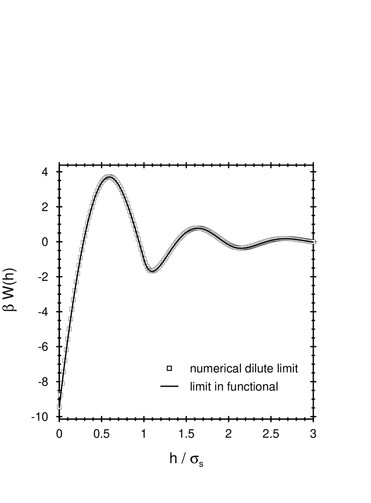
FIG. 1.: Comparison of the depletion potential for a big hard sphere near a planar hard wall, calculated via two different routes. These correspond to taking the dilute limit directly in the functional (solid line), and to taking the dilute limit numerically with a packing fraction of the big spheres of $\eta_{b}=10^{-4}$ ($\square$). In both cases the size ratio is $s=R_{s}/R_{b}=0.1$ and the packing fraction of the small hard spheres is $\eta_{s}=0.3$. $h$ is the separation between the wall and the surface of the big sphere; $\sigma_{s}=2R_{s}$ is the diameter of the small spheres.

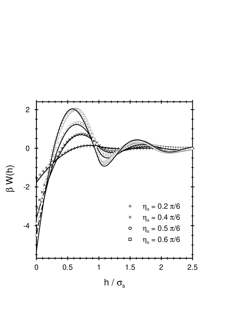
FIG. 2.: The depletion potential between two big hard spheres in a sea of small hard spheres calculated for various packing fractions $\eta_{s}$ of the small spheres and a fixed size ratio $s=0.1$. We compare simulation results (symbols) from Ref. [14] with results from our DFT approach (solid lines). $h$ is the separation between the surfaces of the two big spheres and $\sigma_{s}$ is the diameter of the small spheres.

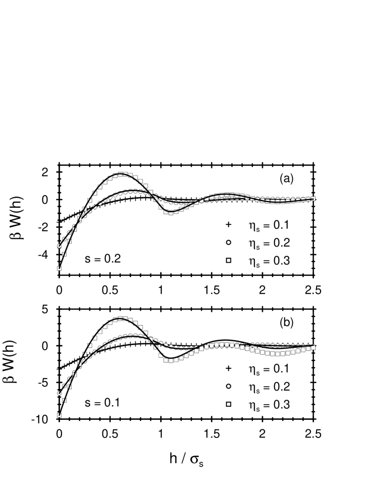
FIG. 3.: The depletion potential between a big hard sphere and a planar hard wall calculated for various packing fractions $\eta_{s}$ of the small hard spheres and size ratios $s=0.2$ (a) and $s=0.1$ (b). We compare processed simulation data from Ref. [15] (symbols) with those of our calculations (solid lines). The only significant deviations occur in (b) for $\eta_{s}=0.3$ (see text). $h$ is the separation between the wall and the surface of the big sphere; $\sigma_{s}$ is the diameter of the small spheres.

FIG. 4.: The number density profiles of the two components of a binary hard-sphere mixture near a planar hard wall as obtained from DFT. The reservoir packing fraction of the small spheres is $\eta_{s}=0.3$ and that of the big spheres $\eta_{b}=10^{-4}$. For the three different size ratios $s=0.1$, 0.1333, and 0.2 the profiles of the small spheres (a) are indistinguishable while the profiles of the big spheres (b) differ considerably. The contact values of the density profiles of the big spheres are $\rho_{b}(z=\sigma_{b}^{+})\sigma_{b}^{3}$ = 0.0279, 0.2518, and 2.1814 for $s$=0.2, 0.1333 and 0.1, respectively. $z=0$ denotes the position of the wall and $\sigma_{s}$ is the diameter of the small spheres.

FIG. 5.: The asymptotic decay of the number density profiles of the two components of a binary hard-sphere mixture near a planar hard wall for three different size ratios $s$. The packing fraction of the small spheres is $\eta_{s}=0.3$ and that of the big spheres is $\eta_{b}=10^{-4}$. In each case the natural logarithm of the modulus of the density profile minus the corresponding bulk density is plotted. The upper lines denote the density profiles of the small spheres; these are practically the same for all $s$. The lower lines denote the density profiles of the big spheres and it can be seen that the amplitude of the oscillations does depend on the size ratio $s$. However, for $z/\sigma_{s}\gtrsim 2$ the same characteristic decay length $a_{0}^{-1}$ and wavelength of oscillation $2\pi/a_{1}$ characterize the decay of both density profiles; i.e., for the big and the small spheres (see text). Note that the density profiles in Fig. 4 have been shifted so that here $z$ measures the distance from contact. $\sigma_{s}$ is the diameter of the small spheres.

FIG. 6.: The asymptotic decay of the depletion potentials $W(z)$ for a big hard sphere near a planar hard wall for the same parameters as shown in Fig. 5, i.e., $\eta_{s}=0.3$ and three size ratios $s$. The same decay length $a_{0}^{-1}$ and wavelength $2\pi/a_{1}$ that determine the asymptotic decay of the density profiles determine the decay of $W(z)$ (see text). Only the amplitude of the oscillations depend on $s$. In each case $z$ measures the distance from contact. $\sigma_{s}$ is the diameter of the small spheres.

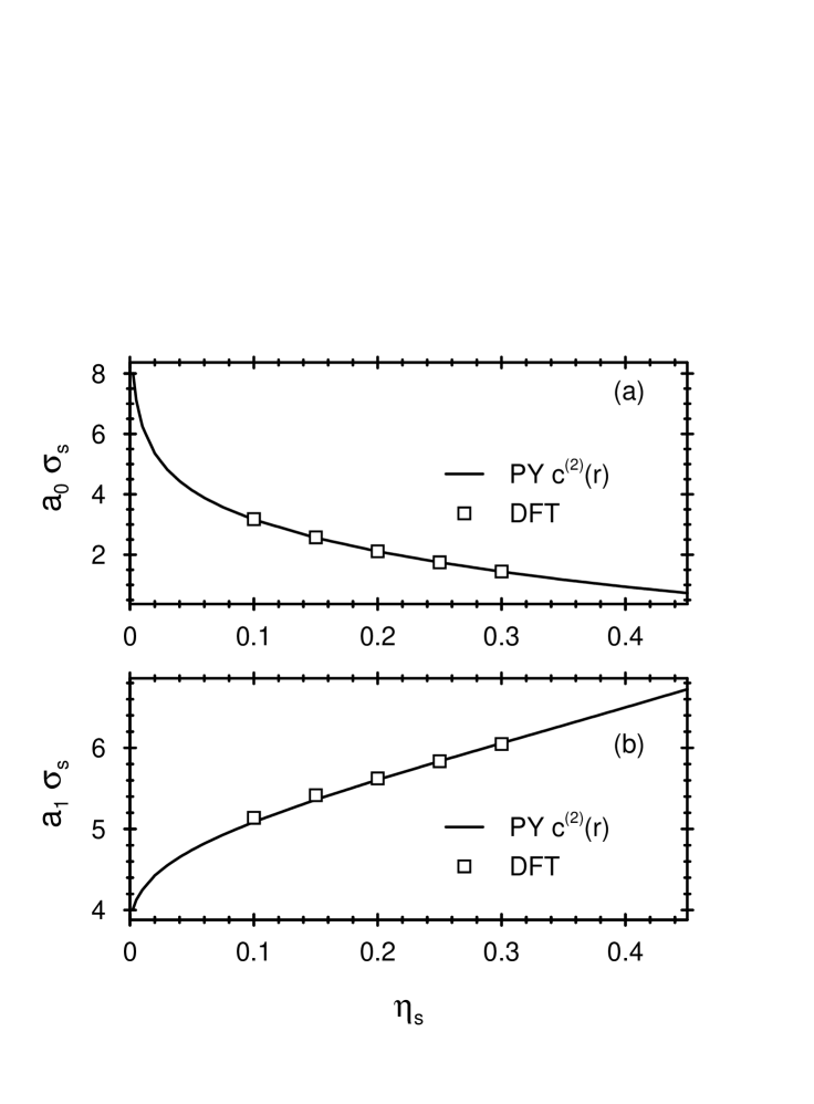
FIG. 7.: Comparison of (a) the inverse decay length $a_{0}$ and (b) the inverse wavelength $(2\pi/a_{1})^{-1}$ as determined from the theory of asymptotic decay of the bulk pairwise correlation [see Eq. (24)] using the Percus-Yevick two body direct correlation function $c^{(2)}_{ss}(r)$ (solid line) with the corresponding results obtained from density profiles calculated using the Rosenfeld functional ($\square$) for hard-sphere fluids near a planar hard wall. $\eta_{s}$ is the packing fraction and $\sigma_{s}$ is the diameter of the small spheres.

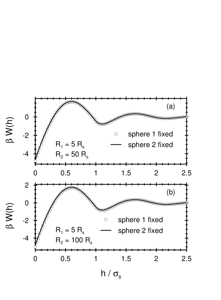
FIG. 8.: The depletion potential between a hard sphere $1$ with radius $R_{1}=5R_{s}$ and a hard sphere $2$ with radius $R_{2}=50R_{s}$ (a) and $R_{2}=100R_{s}$ (b), in a sea of small hard spheres with radius $R_{s}$ and packing fraction $\eta_{s}=0.3$. The solid line denotes the depletion potential calculated by fixing sphere 2 first, so that 2 enters into the calculation as an external potential, whereas the symbols denote the depletion potential obtained with sphere 1 acting as the external potential. The two routes should lead to the same results (see text). $h$ is the separation between the surfaces of the spheres 1 and 2 and $\sigma_{s}=2R_{s}$.

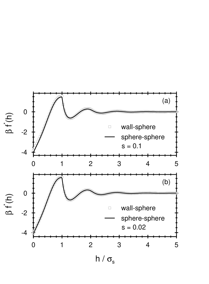
FIG. 9.: The scaled depletion force between two big hard spheres $\beta f^{*}(h)$ = $2\beta F(h)R_{s}^{2}/(R_{b}+R_{s})$ (solid line) and between a single big hard sphere and a planar hard wall $\beta f^{*}(h)$ = $\beta F(h)R_{s}^{2}/(R_{b}+R_{s})$ ($\square$) in a sea of small hard spheres at a packing fraction $\eta_{s}=0.3$ for size ratios $s=0.1$ (a) and $s=0.02$ (b). For $s=0.02$, the scaling relation in Eq. (39) is obeyed almost perfectly. $h$ is the separation between the surfaces of the big spheres or between the wall and the surface of the big sphere. $\sigma_{s}=2R_{s}$ is the diameter of the small spheres.

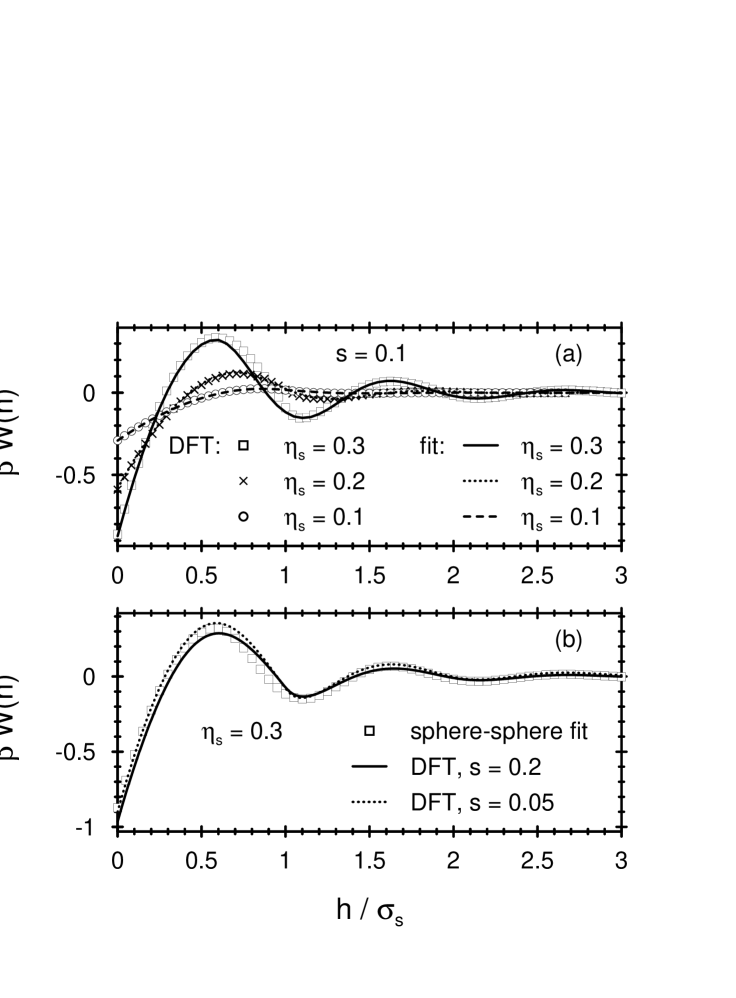
FIG. 10.: (a) Comparison of the scaled wall-sphere depletion potential [Eq. (44)] for various packing fractions $\eta_{s}$ of the small hard spheres and size ratio $s=0.1$ as calculated fully within DFT (symbols) and as given by the parametrization of Eq. (48) (lines). (b) Comparison of the scaled sphere-sphere depletion potentials for a packing fraction $\eta_{s}=0.3$ and size ratios $s=0.2$ and $s=0.05$ as calculated within DFT (lines) and as given by the parametrization of Eq. (48) ($\square$). Differences between the parametrized results for $s=0.2$ and $s=0.05$ are not visible. $h$ is the separation between the wall and the surface of the big sphere or between the surfaces of the two big spheres. $\sigma_{s}$ is the diameter of the small spheres.

FIG. 11.: The depletion potential between two big hard spheres in a sea of small hard spheres at various values of the small sphere packing fraction $\eta_{s}$ as obtained from the original Rosenfeld functional. In order to mimic the experiment of Ref. [7] the diameters were chosen to be $\sigma_{b}=1.1\mu$m and $\sigma_{s}=0.083\mu$m so that the size ratio is $s=0.0755$. $h$ measures the separation between the surfaces of the big spheres. Note that for display purposes each curve has been shifted downward by a constant amount; $W(h)$ oscillates around zero as $h\to\infty$. The dotted line for $\eta_{s}=0.42$ corresponds to the depletion potential calculated with the modified interpolation form of the Rosenfeld functional [27].

REFERENCES

- [1] S. Asakura and F. Oosawa, J. Chem. Phys. 22, 1255 (1954); A. Vrij, Pure and Appl. Chem. 48, 471 (1976).
- [2] M. Dijkstra, R. Van Roij, and R. Evans, Phys. Rev. Lett. 81, 2268 (1998); ibid 82, 117 (1999); Phys. Rev. E 59, 5744 (1999).
- [3] M. Dijkstra, J.M. Brader, and R. Evans, J. Phys.: Cond. Matter 11, 10079 (1999).
- [4] A.A. Louis, R. Finken, and J.-P. Hansen, Phys. Rev. E. 61, R1028 (2000).
- [5] See, e.g., P.D. Kaplan, L.P. Faucheux, and A.J. Libchaber, Phys. Rev. Lett. 73, 2793 (1994); Y.N. Ohshima et al. Phys. Rev. Lett. 78, 3963 (1997); D.L. Sober and J.Y. Walz, Langmuir 11, 2352 (1995); A. Milling and S. Biggs, J. Colloid Sci. 170, 604 (1995); D. Rudhardt, C. Bechinger, and P. Leiderer, Phys. Rev. Lett. 81, 1330 (1998); R. Verma, J.C. Crocker, T.C. Lubensky, and A.G. Yodh, Phys. Rev. Lett. 81, 4004 (1998).
- [6] A.D. Dinsmore, D.T. Wong, P. Nelson, and A.G. Yodh, Phys. Rev. Lett. 80, 409 (1998).
- [7] J.C. Crocker, J.A. Matteo, A.D. Dinsmore, and A.G. Yodh, Phys. Rev. Lett. 82, 4352 (1999).
- [8] Y. Mao, M.E. Cates, and H.N.W. Lekkerkerker, Physica A 222, 10 (1995).
- [9] B. Götzelmann, R. Evans, and S. Dietrich, Phys. Rev. E 57, 6785 (1998); B. Götzelmann, doctoral thesis, Bergische Universität Wuppertal (1998).
- [10] P. Attard, J. Chem. Phys. 91, 3083 (1989).
- [11] P. Attard and G.N. Patey, J. Chem. Phys. 92, 4970 (1990); P. Attard and J.L. Parker, J. Phys. Chem. 96, 5086 (1992).
- [12] J. Piasecki, L. Bocquet, and J.-P. Hansen, Physica A 218, 125 (1995).
- [13] Y. Rosenfeld, Phys. Rev. Lett. 63, 980 (1989); J. Chem. Phys. 98, 8126 (1993).
- [14] T. Biben, P. Bladon, and D. Frenkel, J. Phys.: Condens. Matter 8, 10799 (1996).
- [15] R. Dickman, P. Attard, and V. Simonian, J. Chem. Phys. 107, 205 (1997).
- [16] B. Götzelmann, R. Roth, S. Dietrich, M. Dijkstra, and R. Evans, Europhys. Lett. 47, 398 (1999); R. Roth, doctoral thesis, Bergische Universität Wuppertal (1999).
- [17] R. Roth, B. Götzelmann, and S. Dietrich, Phys. Rev. Lett 83, 448 (1999).
- [18] C. Bechinger, D. Rudhardt, P. Leiderer, R. Roth, and S. Dietrich, Phys. Rev. Lett. 83, 3960 (1999).
- [19] J.R. Henderson, Mol. Phys. 50, 741 (1983); see in particular Eqs. (12) and (18).
- [20] R. Evans, Adv. Phys. 28, 143 (1979).
- [21] S. Melchionna and J.-P. Hansen, preprint Cambridge University (2000).
- [22] R. Evans, R.J.F. Leote de Carvalho, J.R. Henderson, and D.C. Hoyle, J. Chem. Phys. 100, 591 (1994).
- [23] R. Evans, J.R. Henderson, D.C. Hoyle, A.O. Parry, and Z.A. Sabeur, Mol. Phys. 80, 755 (1993).
- [24] Y. Rosenfeld, Phys. Rev. E 50, R3318 (1994); Mol. Phys. 86, 637 (1995).
- [25] J.A. Cuesta, Phys. Rev. Lett. 76, 3742 (1996).
- [26] Y. Rosenfeld, M. Schmidt, H. Löwen, and P. Tarazona, J. Phys.: Condens. Matter 8, L577 (1996); Phys. Rev. E 55, 4245 (1997).
- [27] Various modifications of the original Rosenfeld functional are proposed in Ref. [26]. While all the modified functionals predict the freezing transition of the pure hard-sphere fluid, we employ those that have the same bulk fluid properties as the original functional. In particular the functionals we choose correspond to the same (Percus-Yevick) free-energy density and pair direct correlation functions. This implies that the inverse decay length and the wavelength of the asymptotic decay of the depletion potential [see Eqs. (27) and (29)] are the same for each choice of the functional. In our calculations we used the antisymmetrized version with [see Eq. (27) in Ref. [26]] and the interpolation form [Eq. (28) in Ref. [26]] which interpolates between the original Rosenfeld and a form which is exact in the zero-dimensional limit.
- [28] T. Biben, private communication.
- [29] R. Roth and S. Dietrich, preprint cond-mat/0003290 (2000).
- [30] B.V. Derjaguin, Kolloid-Z. 69, 155 (1934).
- [31] N.F. Carnahan and K.E. Starling, J. Chem. Phys. 51, 635 (1969).
- [32] H. Reiss, H.L. Frisch, E. Helfand, and J.L. Lebowitz, J. Chem. Phys. 32, 119 (1960).
- [33] A similar change in sign of at a value of lying between 0.3 and 0.4 was found in a scaled particle theory of the depletion potential for a size ratio ; see D. Corti and H. Reiss, Mol. Phys. 95,269 (1998).
- [34] The repulsive contributions reported in Ref. [18] are associated with dispersion forces.
- [35] A. González, J.A. White, F.L. Román, and R. Evans, J. Chem. Phys. 109, 3637 (1998).
- [36] L.J.D. Frink and A.G. Salinger, J. Comp. Phys. 159, 407 (2000); ibid 159 425 (2000).
- [37] H.H. von Grünberg and R. Klein, J. Chem. Phys. 110, 5421 (1999).
- [38] R. Evans in Fundamentals of Inhomogeneous Fluids, edited by D. Henderson (Dekker, New York, 1992) p.85.
- [39] We suspect that several integral-equation studies of hard-sphere mixtures have focused on states lying actually in the two-phase region.