$\stackrel{{\scriptstyle\rm\textstyle SU{-}4240{-}709\quad}}{{\rm\textstyle\quad}}$
The Geometrical Structure of 2D Bond-Orientational Order

We study the formulation of bond-orientational order in an arbitrary two dimensional geometry. We find that bond-orientational order is properly formulated within the framework of differential geometry with torsion. The torsion reflects the intrinsic frustration for two-dimensional crystals with arbitrary geometry. Within a Debye-Huckel approximation, torsion may be identified as the density of dislocations. Changes in the geometry of the system cause a reorganization of the torsion density that preserves bond-orientational order. As a byproduct, we are able to derive several identities involving the topology, defect density and geometric invariants such as Gaussian curvature. The formalism is used to derive the general free energy for a 2D sample of arbitrary geometry, both in the crystalline and hexatic phases. Applications to conical and spherical geometries are briefly addressed.

1 Introduction

According to the KTNHY theory [1, 2, 3], two-dimensional melting in the plane is a two stage defect-driven process involving continuous crystalline-to-hexatic and hexatic-to-fluid transitions. The intermediate hexatic phase is characterized by quasi-long-range bond orientational order and positional disorder. In a wide variety of settings one may expect to encounter geometries more general than the plane. In the theory of membranes the geometry itself fluctuates. External forces may act to bend the geometry to some fixed curved surface. This raises the challenging problem of generalizing the established KTNHY theory to substrates with some arbitrary geometry. In this paper we discuss a complete geometrical formulation of bond-orientational order [4] (hexatic and crystalline) that provides a framework in which the interaction of defects, geometry and topology are easily formulated.

To begin, consider a hypothetical flat monolayer displaying bond-orientational order at zero temperature. Bonds may be represented as six vectors at each point of the plane, with a relative angle of $\frac{\pi}{3}$. The six vectors at any given point of the plane are parallel to those at any other point. In other words, if we know the vectors at some point we can reconstruct the vectors at any other point by parallelism. Imagine now adiabatically deforming the plane of the monolayer to an arbitrary curved surface. Intuitively we would expect the bond-orientational order to be stable to this deformation. The curvature of the monolayer, however, now implies an associated Gaussian curvature. As well known from differential geometry there is no intrinsic notion of parallelism on curved surfaces. To define parallel transport we require a rule specified via a connection. In general parallel transport of a vector between two points will depend on the path. For our problem this means that the bond angle at an arbitrary point on the surface has no path-independent meaning. For the standard choice of connection (the Levi-Civita connection) the bond angle at some point reached by two distinct paths from a reference point will depend on the total Gaussian curvature enclosed by the paths. This sensitive dependence on the path suggests that bond-orientational order is incompatible with any curved geometry.

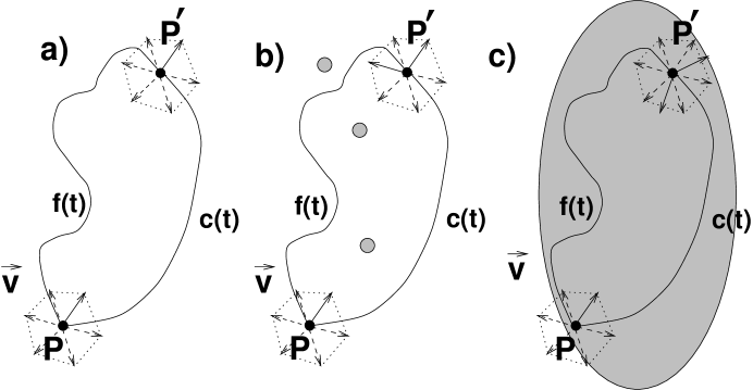
Figure 1: The result of parallel transport of ${\bf V}$ from $P$ to $P^{\prime}$ a) phase with no disclinations: the result is path-independent b) phase with a few isolated disclinations, marked as grey spots: the result may differ by an angle of $\frac{\pi}{3}$ but bond-orientational order is preserved c) isotropic fluid phase: parallel transport is completely ambiguous.

This mathematical argument, however, contradicts our intuition that bond-orientational order should be stable to deformation of the surface. This suggests that a more physical connection exists for defining bond-orientational order on curved surfaces. To see this note that bond-orientational order very generally implies the existence of a frame of six bonds forming a $\frac{\pi}{3}$ angle at each point of the sample. Given this data we can define a path-independent parallel transport in the following way. Take a vector ${\bf V}$ at point $P$. This forms a certain angle with the frame. Now we can transport ${\bf V}$ to the point $P^{\prime}$ by demanding that ${\bf V}$ forms the same angle to the given frame at $P^{\prime}$. By construction this physical parallel transport does not depend on the path and is therefore unambiguous .

Clearly the connection that corresponds to the parallel transport defined above must be different from the standard Levi-Civita connection. We will argue below that the mathematical realization of this physical connection appropriate for defining bond-orientational order involves a new degree of freedom, a geometrical quantity called torsion. The difference angle between two parallel transported vectors will depend on the enclosed curvature of the new connection with torsion. This connection may be tuned to be curvature-free so that parallel transport is path-independent, as desired.

Although torsion may appear at this stage as merely a mathematical trick, a number of authors [7] have identified torsion as necessary for describing a system with a high density of dislocations, such as in the hexatic phase. This is certainly the case if the density of dislocations is well approximated by a continuous density, corresponding to the Debye-Huckel approximation. We will see more generally, however, that torsion accounts for the intrinsic frustration of a 2d configuration on a curved surface.

This curvature of the connection with torsion also has a clear physical interpretation as being proportional to the density of disclinations. Raising the temperature slightly will excite disclinations. Although the zero curvature condition is violated, it is such that parallel transport is ambiguous only up to an angle $\pi/3$, and the hexatic order is preserved. As the temperature is raised further the growing density of free disclinations will eventually melt the hexatic to a fluid. The high density of disclinations in this phase may be represented by a continuous disclination density. In this case the parallel transported bond angle is completely ambiguous, which is equivalent to saying that bond angles are meaningless in the isotropic fluid phase.

The organization of the paper is as follows: in the next section we introduce the necessary background in differential geometry, which will also serve to fix our notation. In section 3 we provide the physical interpretation of torsion and derive some general relations involving the geometry, the defect density and the torsion. In section 4 we reformulate the case of a simple flat monolayer in terms of the new formalism: this is easily generalized to an arbitrary geometry. We end the paper with some conclusions. In the appendix we treat the example of a cone displaying hexatic order as an explicit application of our formalism.

2 Differential geometry background

In this section we briefly emphasize those concepts in differential geometry that play a major role in the subsequent analysis. For further details we refer the reader to the literature [8].

2.1 Basic differential geometry

A $D$-dimensional surface embedded in $d$-dimensional Euclidean space is described by $d$-dimensional functions $R^{\alpha}({\bf x})\ ,\alpha=1,\cdots,d$ of $D$ coordinates $x^{\mu}\ ,\mu=1,\cdots D$, with $D=2$ being the physically interesting case.

The fact that the surface is embedded in ${\bf R}^{d}$ provides a natural metric,

$$ds^{2}=g_{\mu\nu}dx^{\mu}\otimes dx^{\nu}\ ,\ g_{\mu\nu}=\partial_{\mu}{\vec{R}}\cdot\partial_{\nu}{\vec{R}}\ .$$ (1)

Introducing the vielbeins, ${e^{a}}_{\mu}$, it is possible to rewrite the previous equation as

$$ds^{2}=\delta_{ab}\vartheta^{a}\otimes\vartheta^{b}\ ,$$ (2)

where $\vartheta^{a}={e^{a}}_{\mu}dx^{\mu}$. It is easy to check that the tangent vectors

$$e_{a}={e^{\mu}}_{a}\frac{\partial}{\partial x^{\mu}}\ ,\ a=1,\cdots,D\ ,$$ (3)

where ${e^{\mu}}_{a}{e^{a}}_{\nu}=g_{\mu\nu}$, define a basis of orthonormal vectors. The dot product of any two vectors ${\bf u}=u^{a}e_{a}$ and ${\bf v}=v^{a}e_{a}$ in tangent space is ${\bf u}\cdot{\bf v}=\delta_{ab}u^{a}v^{b}$, as if the metric were flat. This formalism is called the non-coordinate basis. Hereafter we use the first letters of the Latin alphabet when we work in a non-coordinate basis, and Greek indices for the coordinate basis.

The space of all $r$-dimensional forms of a manifold $M$ $\Omega^{r}(M)$ plays an important role. The metric allows one to define a natural isomorphism, the Hodge-star operator

$$\Omega^{r}(M)\stackrel{{\scriptstyle\ast}}{{\rightarrow}}\Omega^{D-r}(M)\ ,$$ (4)

defined as the linear map which in a non-coordinate acts as

$$\ast(\vartheta^{a_{1}}\wedge\vartheta^{a_{2}}\wedge\cdots\wedge\vartheta^{a_{r}})=\frac{1}{(D-r)!}{\epsilon^{a_{1}\cdots a_{r}}}_{a_{r+1}\cdots a_{D}}(\vartheta^{a_{r+1}}\wedge\cdots\wedge\vartheta^{a_{D}}),$$ (5)

where $\epsilon^{12\cdots D}=1$. We may define an inner product in $\Omega^{r}(M)$. If $\omega=\frac{1}{r!}\omega_{a_{1}\cdots a_{r}}\vartheta^{a_{1}}\wedge\cdots\vartheta^{a_{r}}$ and $\nu=\frac{1}{r!}\nu_{a_{1}\cdots a_{r}}\vartheta^{a_{1}}\wedge\cdots\vartheta^{a_{r}}$

$$(\omega|\nu)=\int_{M}\omega\wedge\ast\nu=\int_{M}\omega_{a_{1}\cdots a_{r}}\nu^{a_{1}\cdots a_{r}}\sqrt{|g|}dx^{1}\cdots dx^{D}\ ,$$ (6)

the integral being over the whole manifold $M$.

The adjoint $d^{\dagger}$ of the exterior derivative is defined as the linear operator satisfying

$$(d\alpha|\beta)=(\alpha|d^{\dagger}\beta)\ .$$ (7)

It is an easy exercise to check that $d^{\dagger}=(-1)^{Dr+D+1}\ast d\ast$. The Laplacian is the operator

$$\Delta=dd^{\dagger}+d^{\dagger}d\ .$$ (8)

Let us recall that the Laplacian is independent of the connection.

2.2 Connections

A connection on a manifold $M$ specifies how tensors are transported along a curve. It allows one to define a covariant derivative $\nabla_{\mu}$ on a vector field $U$,

$$\nabla_{\mu}U^{\nu}=\partial_{\mu}U^{\nu}+\Gamma^{\nu}_{\mu\sigma}U^{\sigma}\ ,$$ (9)

where $\Gamma^{\nu}_{\mu\sigma}$ are the connection coefficients. The parallel transport of a vector $V^{\mu}$ along a curve $c^{\mu}$ is fixed by demanding that is be covariantly constant:

$$\nabla_{c}V^{\mu}=\frac{dc^{\nu}(t)}{dt}\nabla_{\nu}V^{\mu}=0\ .$$ (10)

It is convenient to define the connection coefficients in a non-coordinate basis:

$$\nabla_{a}e_{b}={\Gamma^{c}}_{ab}e_{c}\ ,$$ (11)

and a connection one-form via

$${\omega^{a}}_{b}={\Gamma^{a}}_{cb}\vartheta^{c}\ .$$ (12)

We consider only metric connections that preserve the norm of a vector under parallel transport, a property called metric compatibility. This property constrains the connection one-form to satisfy

$${\omega^{a}}_{b}=-{\omega^{b}}_{a}\ ,$$ (13)

which in $D=2$ further simplifies to ${\omega^{a}}_{b}=-{\epsilon^{a}}_{b}\Omega$, $\Omega=\Omega_{a}\vartheta^{a}$. Connection coefficients do not transform as a tensor but it is possible to construct two tensorial objects out of them, the torsion and the curvature. For the sake of completeness, we write them acting on vector fields $X,Y$,

$$T(X,Y) = \nabla_{X}Y-\nabla_{Y}X-[X,Y]$$

$$R(X,Y) = \nabla_{X}\nabla_{Y}-\nabla_{Y}\nabla_{X}-\nabla_{[X,Y]}$$ (14)

Expressions turn out simpler in a non-coordinate basis. Defining torsion and curvature 2-forms by

$$T^{a} = \frac{1}{2}{T^{a}}_{bc}\vartheta^{b}\wedge\vartheta^{c}$$

$${R^{a}}_{b} = \frac{1}{2}{R^{a}}_{bcd}\vartheta^{c}\wedge\vartheta^{d}\ ,$$ (15)

they are related to the connection one-form by Cartan’s structure equations, which read for the case $D=2$,

$$T^{a} = d\vartheta^{a}-\Omega\wedge\vartheta^{b}{\epsilon^{a}}_{b}\$$ (16)

$$\frac{1}{2}{\epsilon_{a}}^{b}{R^{a}}_{b} = d\Omega\ .$$

Recall that the curvature 2-form is locally an exact form. The expressions in the coordinate basis follow easily from those in the non-coordinate basis from the tensorial nature of curvature and torsion, namely ${T^{\mu}}_{\nu\rho}={e^{\mu}}_{a}{e^{b}}_{\nu}{e^{c}}_{\rho}{T^{a}}_{bc}$ and ${R^{\mu}}_{\nu\rho\sigma}={e^{\mu}}_{a}{e^{b}}_{\nu}{e^{c}}_{\rho}{e^{d}}_{\sigma}{R^{a}}_{bcd}$.

2.3 Some global considerations

The global structure of the manifold places important constraints on the differential geometry of the surface. From Eq. 16 the curvature 2-form is locally an exact form, but that is not the case globally. For a manifold without boundaries, integrating over the whole manifold we have

$$\int_{M}\frac{1}{2}{\epsilon_{a}}^{b}{R^{a}}_{b}=2\pi\sum_{\alpha}Ind_{\alpha}=2\pi\chi\ ,$$ (17)

where $Ind$ are the indices of the vector field associated with $\Omega$ and $\chi$ is the Euler characteristic of the manifold. If $R$ is the Riemannian curvature this is the usual Gauss-Bonnet theorem.

3 The geometry of bond-orientational order

We now consider a two-dimensional sample exhibiting bond-orientational order and forming an arbitrary shape in d-dimensional space, specified by the embedding $R^{\alpha}({\bf x})$. Within the sample, distances are measured according to the metric Eq. 1.

The main feature of connections with non-vanishing torsion (non-symmetric connections) is that infinitesimal reference vectors fail to close when parallel transported along each other, as illustrated in Fig. 2. If a crystal is forced to lie on an arbitrary geometry, the atoms in the crystal cannot be all equally separated by a distance $a$. This implies that parallel transport along the bonds joining the nearest-neighbors will fail to close, as shown in Fig. 2. Thus we see that torsion is related to the intrinsic frustration experienced by a 2D crystal on an arbitrary surface.

In the hexatic phase there is a similar interpretation of torsion, except that there will be a large number of dislocations. This is specified by a Burgers vector density

$${\bf b}({\bf x})=\frac{1}{\sqrt{g}({\bf x})}\sum_{i}{\bf b}_{i}^{L}\delta({\bf x}_{i}-{\bf x})$$ (18)

where ${\bf b}_{i}^{L}$ is the microscopic Burgers vectors with origin at point ${\bf x}_{i}$. In a highly dislocated medium, the discreteness of the Burgers vector density ${\bf b}(x)$ may be approximated by a continuous vector density, the so-called Debye-Huckel approximation.

Figure 2: Parallel Transport in the presence/absence of Torsion.

The density ${\bf b}(x)$ is, in fact, directly related to the torsion invariant appearing in Eq. 2.2, as noted by several authors [7]. The torsion two-form is

$$T^{a}=v^{a}\vartheta^{1}\wedge\vartheta^{2}=v^{a}\Omega_{M}\ ,$$ (19)

where $\Omega_{M}=\sqrt{|g|({\bf x})}dx^{1}\wedge dx^{2}$ is the volume form. Since $v^{a}$ is a vector it can be written in a coordinate basis $v^{\mu}={e^{\mu}}_{a}v^{a}$. Its geometric interpretation is illustrated in Fig. 2. Let us assume non-zero torsion at point $A$. Consider the vector $\overline{AC}$ and parallel transport it along vector $\overline{AB}$, the resulting vector is $\overline{BD^{\prime}}$. If we parallel transport vector $\overline{AB}$ along $\overline{AC}$ we get $\overline{CD^{\prime\prime}}$. Using the parallel transport Eq. 10 and Eq. 9, we may write to lowest order

$$\overline{D^{\prime\prime}D^{\prime}}^{\mu}=\left\{\Gamma^{\mu}_{\sigma\nu}-\Gamma^{\mu}_{\nu\sigma}\right\}\overline{AB}^{\sigma}\overline{AC}^{\nu}=v^{\mu}\times\mbox{Area of the region ($ABD^{\prime}D^{\prime\prime}C)$}.$$ (20)

If ${\bf v}=0$ then $D^{\prime}=D^{\prime\prime}=D$ and the parallelogram closes.

It is clear from the previous geometrical argument that torsion is related to the continuous density of Burgers vector by

$${\bf b}({\bf x})={\bf v}({\bf x})\ ,$$ (21)

or $T^{a}=b^{a}\Omega_{M}$, in a non-coordinate basis. A highly dislocated media physically is represented geometrically by a surface endowed with a connection with torsion [7].

Clearly then torsion is a necessary ingredient in a geometrical description of bond-orientational order, as it allows a connection form from which the bond angle is constructed by parallel transport. This interpretation of torsion is completely general. In the Debye-Huckel limit we have the additional identification of the torsion with the dislocation density.

In the absence of free disclinations we pointed out that this result should be independent of the path chosen. This in turn translates into the mathematical requirement of vanishing curvature 2-form

$${R^{a}}_{b}=0\ .$$ (22)

This is a local condition, not always possible to fulfill globally, as for example in the case of spherical topology. Anyway, Eq. 22 is fulfilled everywhere for the case of a sample having the topology of a plane.

In this regime, the Cartan structure equations Eq. 16 read

$$T^{a} = d\vartheta^{a}-\Omega\wedge\vartheta^{b}{\epsilon^{a}}_{b}\ ,$$ (23)

$$0 = d\Omega\ ,$$

The last equation implies $\Omega=d\theta$, where $\theta({\bf x})$ is a 0-form, a function. Let us interpret its physical meaning. The equation of parallel transport Eq. 10 reads

$$\frac{dV^{a}}{dt}-\Omega_{\mu}\frac{dc^{\mu}}{dt}{\epsilon^{a}}_{b}V^{b}=0\ ,$$ (24)

where $c^{\mu}(t)$ parametrizes a curve in the surface joining the points $P$ and $P^{\prime}$.

$$V_{\pm}(P^{\prime})=V_{\pm}(P)e^{-i\int_{c}\Omega_{\mu}dx^{\mu}}\ ,$$ (25)

In the hexatic phase with no free disclinations, Eq. 23 implies

$$V_{\pm}(P^{\prime})=V_{\pm}(P)e^{-i\theta(P^{\prime})}\ ,$$ (26)

where $V_{\pm}=V^{1}\pm iV^{2}$ and $\theta(P)=0$. This parallel transport id manifestly path independent and $\theta$ clearly is the bond angle at point $P^{\prime}$. Dragging $P^{\prime}$ along the entire surface and performing the parallel transport Eq. 26 we can unambiguously construct the bond angle at any point from the knowledge of the bond angle at $P$. We have succeeded in giving a precise mathematical formulation of the heuristic zero temperature experiment performed in the introduction.

3.1 Introduction of free disclinations

The sample may also contain some free disclinations, either as a result of thermal fluctuations or because topological constraints force them to appear. In either case, the parallel transport can only be defined modulo an angle of $\frac{\pi}{3}$. The system responds to the raising of the temperature by generating curvature, but only via defects that preserve overall hexatic order, the disclinations. In this way, the curvature is directly related to the density of disclinations [7].

From these arguments, it is clear that a finite density of $N$ free disclinations is represented as

$$\frac{1}{2}{\epsilon_{a}}^{b}{R^{a}}_{b} = s({\bf x})\Omega_{M}$$

$$s({\bf x}) = \frac{\pi}{3}\frac{1}{\sqrt{|g|}}\sum_{j=1}^{N}q_{j}\delta({\bf x}-{\bf x}_{j})\ ,$$ (27)

where $q_{i}$ may be $+1$ (a five-fold disclination) or $-1$ (a seven-fold disclination). Higher integer charges are also possible although rarely need to be considered. If the surface is closed, we can integrate the previous equation over the whole manifold. With the aid of the Gauss-Bonnet theorem Eq. 17 we find

$$\sum_{j=1}^{N}q_{j}=6\chi.$$ (28)

This shows that, apart from the torus with $\chi=0$, closed manifolds always contain a certain number of free disclinations.

With free disclinations, the Cartan structure equations (Eq. 16) become

$$T^{a} = d\vartheta^{a}-\Omega\wedge\vartheta^{b}{\epsilon^{a}}_{b}\ ,$$

$$d\Omega = s({\bf x})\Omega_{M}\ .$$ (29)

Away from the actual location of the disclinations $\Omega=d\theta$, but now it is generally impossible for $\theta$ to be defined as a continuous function. It is easy to check that a vectors parallel transported from point $P$ to $P^{\prime}$ following two different paths ${\bf c}(t)$ and ${\bf f}(t)$ paths (see Fig. 1) differ by an angle $\psi$

$$\psi=\frac{\pi}{3}\sum_{j}q_{j}\ ,$$ (30)

where $j$ runs over all charges within the region enclosed by the two paths. The ambiguity is a multiple of $\frac{\pi}{3}$ and as expected hexatic order is preserved. Mathematically we have a connected manifold with a $Z_{6}$ holonomy. Disclinations may be regarded as orbifolds.

Generally, we will write

$$\Omega=d\theta+\Omega_{sing}\ ,$$ (31)

explicitly displaying the bond angle $\theta$ and a a singular part, obviously corresponding to a vortex contribution. This is nothing but the procedure of separating a regular part and a singular part in the standard treatment of the XY model [9].

There is more information encoded in the Cartan structure equations (Eq. 16). First of all, the Levi-Civita connection is obtained imposing the vanishing of torsion,

$$d\vartheta^{a}-\Omega^{L}\wedge\vartheta^{b}{\epsilon^{a}}_{b}=0\ ,$$ (32)

where $\Omega^{L}$ is the connection form of the Levi-Civita connection. We have the important relation

$$d\Omega^{L}=\frac{1}{2}{\epsilon^{a}}_{b}{R_{a}^{G}}^{b}=K({\bf x})\Omega_{M}\ ,$$ (33)

where ${R_{a}^{G}}^{b}$ is the standard Riemann tensor two-form and $K({\bf x})$ is the Gaussian curvature of the surface. Using this relation in Eq. 3.1

$$\Omega^{L}\wedge\vartheta^{b}{\epsilon^{a}}_{b}-\Omega\wedge\vartheta^{b}{\epsilon^{a}}_{b}=T^{a}\ .$$ (34)

Introducing the Burgers form $b=b_{a}({\bf x})\vartheta^{a}=b_{\mu}({\bf x})dx^{\mu}$, together with Eq. 21, this may be rewritten as

$$b=-\Omega+\Omega^{L}\ .$$ (35)

This is a very important equation. It relates the bond angle, computed from the actual connection $\Omega$ as indicated in Eq. 25, to the distribution of dislocations and to the Gaussian curvature of Eq. 33. We can make this statement more apparent by applying the exterior derivative to Eq. 35, and using Eqs. 3.1 and  33:

$$K({\bf x}) = s({\bf x})+\frac{1}{\sqrt{|g|}}\epsilon^{\mu\nu}\partial_{\mu}b_{\nu}({\bf x})$$ (36)

$$\frac{3}{\pi}K({\bf x}) = \frac{1}{\sqrt{|g|}}\sum_{j=1}^{N}q_{j}\delta({\bf x}-{\bf x}_{j})+\frac{3}{\pi}\frac{1}{\sqrt{|g|}}\epsilon^{\mu\nu}\partial_{\mu}b_{\nu}({\bf x})\ .$$ (37)

Note that the coordination number of an atom $n_{i}$, the number of nearest-neighbors, is given by

$$6-n_{i}=q_{i}=\int_{\Sigma}du\sqrt{g}\frac{1}{\sqrt{|g|}}\sum_{j=1}^{N}q_{j}\delta({\bf x}-{\bf x}_{j})=\frac{3}{\pi}\int_{\Sigma}du\sqrt{g}K-\frac{3}{\pi}\int_{\partial\Sigma}b_{\mu}dx^{\mu}\ ,$$ (38)

where $\Sigma_{i}$ is a small region around the atom. This result contains an additional surface term when compared with the existing literature [10, 11]. This surface term will only vanish if defects successfully fully screen out the Gaussian curvature. As we will see in Eq. 59, this is the condition that minimizes the energy of the model. So, at very low temperatures, the surface term will be small.

Comparing Eq. 37 with [11], there is a somewhat disturbing factor $\frac{3}{\pi}$ in the last term. In a fine grained description of the model, one regards a dislocation as a composite object, a tightly bound pair of opposite disclinations (see Fig. 3). Defining the dipole moment ${\bf p}$ as

$$p^{\mu}=\frac{3}{\pi}{\epsilon^{\mu}}_{\nu}b^{\nu}\ ,$$ (39)

where $b^{\nu}$ is the microscopic Burgers vector, we can Taylor expand the density of two free disclinations of opposite charge as

$$\frac{\pi}{3}\left\{\delta({\bf x}+{\bf p})-\delta({\bf x})\right\}=\epsilon^{\mu\nu}b_{\mu}\partial_{\nu}\delta({\bf x})+{\cal O}(a^{2})\ ,$$ (40)

where we neglect higher order terms in the lattice spacing $a$. The right hand side of this last equation corresponds exactly to an isolated dislocation. The factor $\frac{3}{\pi}$ is the slight displacement of the center of the disclinations necessary to render the right dislocation density Eq. 40. As a byproduct, we derive the result that the dipole moment ${\bf p}$ is perpendicular to the microscopic Burgers vector, a result which is also apparent from Fig. 3.

Figure 3: A dislocation as a tightly bound disclination pair. The dotted line is the Burgers circuit. It is apparent that the dipole moment ${\bf p}$ is perpendicular to the Burgers vector ${\bf b}$.

For our purposes, however, it will be more convenient to use Eq. 35 in combination with Eq. 31, which yields

$$b=-d\theta-\Omega_{sing}+\Omega^{L}\ .$$ (41)

This completes our geometrical development of the structure of bond-orientational order.

4 The properties of the hexatic phase

The previous section was somewhat formal. We derived some general results valid in the presence of bond-orientational order. Further progress requires making additional physical assumptions about the interactions of dislocations and disclinations with the underlying geometry and topology.

For the simplest case of a flat monolayer a free energy was proposed in [1, 2] (see [3] for a review). We now examine this proposal within the framework of the geometric formalism developed here. We use a completely covariant language with the aid of the mathematical concepts sketched in Sec. 2. Although this is not necessary for the case of flat space, it is directly applicable to general geometries.

4.1 Debye-Huckel approximation on a flat monolayer

On a flat monolayer, the metric of Eq. 1 is the standard Euclidean metric

$$ds^{2}=dx^{2}+dy^{2}\ .$$ (42)

In this case $\vartheta^{1}=dx$ and $\vartheta^{2}=dy$.

Let us first treat the simpler case of vanishing free disclination density. The bond angle as a function of the Burgers vector density is found by inverting Eq. 41:

$$\theta({\bf x})=\partial_{\mu}(\frac{1}{\Delta}b_{\mu})=-\frac{1}{2\pi}\int d{\bf x^{\prime}}\frac{{\bf b}({\bf x}^{\prime})({\bf x-x^{\prime}})}{|{\bf x-x^{\prime}}|^{2}}\ ,$$ (43)

where $\frac{1}{\Delta}=1/(2\pi)\log(|x-x^{\prime}|)$. This result is in agreement with the results in [1, 2, 3]. We emphasize here that this this result follows from the Cartan structure equations alone, with no further physical assumptions. It provides a non-trivial consistency check for our geometrical interpretation of the hexatic phase.

Additional constraints follow from Eq. 36. With no free disclinations it implies

$$db=0\Longleftrightarrow\epsilon^{\mu\nu}\partial_{\mu}b_{\nu}=0\ .$$ (44)

Geometry thus constrains the Burgers vector distribution ${\bf b}({\bf x})$ to be irrotational.

The free energy of the crystal, within a Debye-Huckel approximation, was derived in [1, 2]:

$${\cal H}/T=\frac{K_{B}}{2}(db|\frac{1}{\Delta^{2}}db)+\frac{E_{c}a^{2}}{T}(b|b)\ ,$$ (45)

where the inner product between forms was defined in Eq. 6 and the Laplacian in Eq. 8. $K_{B}$ is the 2-dimensional Young modulus, $a$ is the original lattice spacing and $E_{c}$ the core energy of a single dislocation. The RG recursion relations of the 2d KTNHY melting transition [1] imply that in the hexatic phase

$${\rm lim}_{{\bf p}\rightarrow 0}K_{B}({\bf p})=0\ .$$ (46)

If now we consider the bond angle as the fundamental variable, Eq. 41 and Eq. 44 imply a simple $XY$ model for the energy of the bond angle variable

$${\cal H}/T=\frac{K_{A}}{2}\int\partial_{\mu}\theta\partial^{\mu}\theta\ ,$$ (47)

with hexatic stiffness $K_{A}=\frac{2E_{c}a^{2}}{T}$ [1, 2].

The irrotationality of ${\bf b}$ is a general constraint to be satisfied in any hexatic regime with vanishing free disclination density. It has additional consequences. We already noted that a dislocation may be regarded as a tightly bound disclination pair. The dipole vector ${\bf p}$, defined in Eq. 39, is perpendicular to the Burgers vector ${\bf b}$. If we consider a closed loop ${\cal C}$, we can compute the circulation for ${\bf p}$

$$\int_{\cal C}{\bf p}d{\bf s}=\int_{\cal C}\epsilon^{\mu\nu}b_{\nu}dx_{\mu}=\int_{\Sigma}dxdy\Delta\theta\ ,$$ (48)

where $\Sigma$ is the two dimensional region enclosed by the closed curve ${\cal C}$. The resultant integral is generally not zero. This means that dipoles form grain boundaries of consecutive fives and sevens. If there are no free disclinations these strings cannot self-intersect.

In the presence of free disclinations, Eq. 44 gets modified to

$$db=sdx\wedge dy\Longleftrightarrow\epsilon^{\mu\nu}\partial_{\mu}b_{\nu}({\bf x})=s({\bf x})\ .$$ (49)

The free energy for the bond angle variable now reads

$${\cal H}/T=\frac{K_{B}}{2}(s|\frac{1}{\Delta}s)+\frac{K_{A}}{2}(d\theta+\Omega_{sing}|d\theta+\Omega_{sing})\ .$$ (50)

The first term leads to a strong binding of free disclinations, since it corresponds to a $|{\bf x}|^{2}\ln|{\bf x}|$ disclination-disclination interaction . Recalling Eq. 46, however, we see that this term is absent. The long-wavelength description of the hexatic phase is given by the standard XY model [1].

The hexatic phase can be characterized by the correlator [12]

$$C({\bf r})=\langle\sigma({\bf r})\sigma({\bf 0})\rangle\ ,$$ (51)

with

$$\sigma({\bf r})=\sum_{l}{\rm Ind}_{l}\delta^{2}({\bf r}-{\bf R}_{l})=\frac{1}{2\pi}s({\bf x})\ ,$$ (52)

where ${\rm Ind}_{l}$ is the index of the order parameter. The last identity follows from the definition of the index of a vector field. The order parameter Eq. 51 is thus the correlation function of the free disclination density, the hexatic curvature. To lowest order in the fugacity, we have in the hexatic phase

$$\langle s({\bf x})s({\bf 0})\rangle\sim\frac{y^{2}}{|{\bf x}|^{\eta}}\ ,$$ (53)

where $y$ is the fugacity of the vortices. In the isotropic liquid phase [12]

$$\langle s({\bf x})s({\bf 0})\rangle\sim e^{-\frac{|{\bf x}|}{\xi}},$$ (54)

where $\xi\sim e^{\frac{a}{T-T_{c}}}$ is the correlation length of the model.

4.2 Hexatic order in an arbitrary geometry

In the previous section we recast standard results for a flat monolayer in the geometric framework developed in this paper. These results may now be extended directly to the case of an arbitrary geometry. The metric

$$ds^{2}=g_{\mu\nu}dx^{\mu}dx^{\nu}\ ,$$ (55)

takes a general form with metric coefficients given by Eq. 1.

The first step is to find the free energy. This is easily obtained from Eq. 45 using the covariant definition of the operators involved, as described in sect. 2 We start by defining the form

$$\rho({\bf x})=\left\{K({\bf x})-s({\bf x})\right\}\Omega_{M}\ ,$$ (56)

expressing the difference between Gaussian curvature and free disclination density. In Eq. 45 we deliberately wrote the free energy of a simple flat monolayer in terms of the torsion degrees of freedom. It is now extremely simple to generalize it to the case of a general geometry by making use the general relation Eq. 41 that holds for an arbitrary geometry to obtain

$${\cal H}/T=\frac{K_{B}}{8}(\rho|\frac{1}{\Delta^{2}}\rho)+\frac{K_{A}}{2}(d\theta+\Omega_{sing}-\Omega^{L}|d\theta+\Omega_{sing}-\Omega^{L})\ ,$$ (57)

where $\Omega^{L}$ is the connection form of the Levi-Civita connection. This corresponds to the free energy of a 2D crystal on an arbitrary geometry. This result is identical to that obtained by integrating out the in-plane phonons [6] in the absence of free disclinations, and generalizing to include these additional degrees of freedom. The free energy Eq. 57 corresponds interacting dislocations and disclinations in the crystalline phase. At zero temperature, one can substitute the bond orientational order parameter $\theta$ by its minimum value $\theta=\frac{1}{\Delta}\nabla_{\mu}\Omega^{\mu}$, and we get

$${\cal H}/T=\frac{K_{B}}{8}(\rho|\frac{1}{\Delta^{2}}\rho)+\frac{K_{A}}{2}(\rho|\frac{1}{\Delta}\rho)\ .$$ (58)

Free positive disclinations are attracted to positive curvature regions and negative disclinations to negative curvature regions. The ground state is defined by the equation

$$\rho=0\Rightarrow s({\bf x})=K({\bf x})\ .$$ (59)

Defects will arrange themselves to optimally screen out the Gaussian curvature.

As for the case of a flat monolayer (Eq. 46), the hexatic phase requires that in the infrared limit

$$K_{B}=0\ .$$ (60)

The free energy then becomes

$${\cal H}/T = \frac{K_{A}}{2}(d\theta+\Omega_{sing}-\Omega^{L}|d\theta+\Omega_{sing}-\Omega^{L})$$ (61)

$$= \frac{K_{A}}{2}\int d{\bf x}\sqrt{g}g^{\mu\nu}(\partial_{\mu}\theta+\Omega_{sing}-\Omega^{L}_{\mu})(\partial_{\nu}\theta+\Omega_{sing}-\Omega^{L}_{\nu})\ ,$$

which is the hexatic free energy first considered in [6].

It is beyond the scope of this paper to investigate the precise mechanism by which Eq. 60 is implemented in an arbitrary geometry, but we show instead that it is a necessary condition for the hexatic phase to be realized.

In analogy with the flat monolayer, one may compute the order parameter Eq. 51 to lowest order in the fugacity,

$$\langle s({\bf x})s({\bf 0})\rangle = -2\left(\frac{\pi}{3}\right)^{2}y^{2}e^{-\frac{K_{A}}{2}\sum_{{\bf x}_{i}\neq{\bf x}_{j}}\left(\frac{1}{\Delta}\right)_{{\bf x_{i}}{\bf x_{j}}}}e^{K_{A}\sum_{{\bf i}=1}^{2}\int d^{2}{\bf x^{\prime}}\frac{q_{i}}{\Delta}_{{\bf x}{\bf x^{\prime}}}\sqrt{g}K({\bf x})}\ ,$$

which reduces to Eq. 53 in the case of a flat monolayer.

It is worthwhile to recall at this point that if fluctuations in the geometry were allowed, we should include an additional bending rigidity or extrinsic curvature term

$$\frac{{\cal H}_{ex}}{T}=\frac{\kappa}{2}\int d{\bf x}\sqrt{g}{\vec{H}}^{2}\ ,$$ (63)

where ${\vec{H}}$ is the Mean curvature of the surface. In this case we average over all possible fluctuations in geometry. It seems that Dislocations have a finite energy [5] and therefore they proliferate at any temperature, see also [13].

5 Conclusions and Outlook

A full understanding of defects in curved geometries is a challenging subject with many novel features not encountered in the plane. In this paper, we presented a geometrical interpretation of bond-orientational order leading to a variety of relations between the underlying geometry, the topology and the nature of the defects. The formalism developed in this paper has already been applied very successfully to the case of defect arrays in spherical crystals [17]. Further applications are currently being explored. The most challenging open problem may be the generalization of the KTNHY renormalization group flows to fixed or dynamical curved geometries. The spherical crystal itself gives rise to a very rich structure of defects in the ground state [17] and other geometries are very likely to lead to even more novel results.

Acknowledgements The research of M.B. and A.T. was supported by the U.S. Department of Energy under contract No. DE-FG02-85ER40237.

Appendix A The hexatic cone

A sample in the hexatic phase on a template having the geometry of a cone is the simplest case where the present formalism may be applied. It provides an interesting benchmark as the cone has been the subject of much interest [14, 15, 16]. For some range of parameters, an isolated disclination forces the flat monolayer to buckle; a positive disclination is optimally screened by the Gaussian curvature located at the cone. It is more convenient to work in polar coordinates $(r,\psi)$, the metric being

$$ds^{2}=(1+m^{2})dr^{2}+r^{2}d\psi^{2}\ ,$$ (64)

where $m$ is related to the aperture angle of the cone $\zeta$ by $\tan\zeta=\frac{1}{m}$.

One readily finds $\vartheta^{1}=\sqrt{1+m^{2}}dr$, $\vartheta^{2}=rd\psi$. The Levi-Civita connection is $\Omega^{L}=-\frac{1}{\sqrt{1+m^{2}}}d\psi$. The actual hexatic connection is flat, corresponding to a plane

$$\Omega=-d\psi+d\phi\rightarrow\theta(r,\psi)=-\psi+\phi(r,\psi)\ ,$$ (65)

where $\phi$ is regular $\phi(r,\psi+2\pi)=\phi(r,\psi)$ and corresponds to the different Burgers vectors distributions one may have in a cone. The lowest energy solution is $\phi=0$, and this is the only case we consider. The torsion vector distribution may be computed easily,

$${\bf b}({\bf x})=(1-\frac{1}{\sqrt{1+m^{2}}})\frac{1}{r}e_{\psi}\ ,$$ (66)

Torsion vectors are tangent to circles centered at the tip of the cone, as depicted in Fig. 4. It is also illuminating to plot the order parameter, as illustrated in Fig. 4. The parallel transported bond angle is completely insensitive to the Gaussian curvature located at the tip of the cone. As a further cross check, we can compute the hexatic energy for this configuration, using the free energy Eq. 61. Assuming a lattice spacing $a$ as an ultraviolet cut-off and the radius $R$ of the cone as an infrared cut-off, we get

$$E_{hex} = \frac{K_{A}}{2}\int^{R}_{a}\frac{dr}{r}(1+m^{2})^{\frac{1}{2}}\int^{2\pi}_{0}d\psi(-1+\frac{1}{\sqrt{1+m^{2}}})^{2}$$ (67)

$$= \pi K_{A}(1-\frac{1}{\sqrt{1+m^{2}}})^{2}(1+m^{2})^{1/2}\ln\frac{R}{a}\ .$$

This result has already been obtained by other authors [14, 15, 16] by solving the equations of motion for the order parameter and computing the Green’s function. Instead we have obtained it by constructing the order parameter by parallel transport. As a byproduct, we are able to compute the torsion vector distribution in the cone.

Figure 4: Distribution of torsion vectors in the cone. Plot of the order parameter in polar coordinates $(r,\psi)$. The order parameter is the same as in a plane despite the Gaussian curvature located at the tip $T$ of the cone.

If there is an isolated disclination located at the tip of the cone, the hexatic connection is no longer flat, as there is hexatic curvature located at the tip of the cone. Parallel transport is now ambiguous if we encircle the tip of the cone. We get,

$$\Omega=(\frac{q_{i}}{6}-1)d\psi\rightarrow\theta(r,\psi)=(\frac{q_{i}}{6}-1)\psi\ .$$ (68)

Following the same steps as before we obtain a free energy of the form given in Eq. 67.

References

- [1] D.R. Nelson and B.I. Halperin, Phys. Rev. B 19 (1979) 2457.
- [2] A. Young, Phys. Rev. B 19 (1979) 1855.
- [3] D.R. Nelson, in Phase Transitions and Critical Phenomena, Vol. 7, C. Domb and J. Lebowitz (Eds;) Academic, New York (1983).
- [4] For a nice collection of articles, see Bond-Orientational Order in Condensed Matter Systems, K. J. Strandburg (Springer-Verlag, New York, 1992).
- [5] H.S. Seung and D.R. Nelson , Phys. Rev. A 38 (1988) 1005.
- [6] D.R. Nelson and L. Peliti, J. Phys. (Paris) 48 (1987) 1085.
- [7] E. Kroner, in Physics of defects, R. Balian, M. Kleman and J.P. Poirier (Eds.) (Les Houches, 1980; A. Kadic and D.G.B. Edelen, Gauge theory of dislocations and disclinations, Springer-Verlag, Berlin/Heidelberg 1983; H. Kleinert, Gauge Fields in Condensed Matter, Vol. II (World Scientific, Singapore, 1989); M.O. Katanaev and I.V. Volovich, Annals of Physics, NY 216 (1991) 1.
- [8] M. Nakahara, Geometry, Topology and Physics, Graduate student series in Physics, 1991, Adam Hilger Inc.; M. Spivak, A comprehensive Introduction to Differential Geometry, 1979, Publish or Perish Inc; B.A. Dubrovin, A.T. Fomenko and S.P. Novikov, Modern Geometry-Methods and Applications (Springer-Verlag, New York 1984).
- [9] J.M. Kosterlitz and D.J. Thouless, J. Phys. C 6 (1973) 581.
- [10] J.P. Gaspard, R Mosseri and J.F. Sadoc, in The Structure of Non-Crystalline Materials, Ph. Gaskell, X. Parker and Y. Davis (Eds;) Taylor and Francis, London (1982) 550.
- [11] S. Sachdev and D.R. Nelson, J. Phys. C 17 (1984) 5473.
- [12] B. Halperin, in Physics of defects, R. Balian, M. Kleman and J.P. Poirier (Eds.) (Les Houches, 1980).
- [13] F. David, E. Guitter and L. Peliti, J. Phys. (Paris) 48 (1987) 1085.
- [14] E. Guitter and M. Kardar, Europhys. Lett. 13 (1990) 441.
- [15] M. W. Deem and D.R. Nelson, Phys. Rev. E 53 (1996) 2551: arXiv:cond-mat/9512079.
- [16] J.-M. Park and T.C. Lubensky, J. Phys. (Paris) I6 (1996) 493: arXiv:cond-mat/9512113.
- [17] M. Bowick, D.R. Nelson and A. Travesset, Phys. Rev. B62 (2000) 8738: arXiv:cond-mat/9911379.