Reconstructed Rough Phases During Surface Growth

Abstract

Flat surface phases are unstable during growth and known to become rough. This does not exclude the possibility that surface reconstruction order persists in rough growing surfaces, in analogy with so-called equilibrium reconstructed rough phases. We investigate this in the context of KPZ type dynamics, using the restricted solid on solid model with negative mono-atomic step energies. Long range reconstruction order is strictly speaking absent in the thermodynamic limit, but the reconstruction domain walls become trapped at surface ridge lines, and the reconstruction order parameter fluctuates critically with the KPZ dynamic exponent at finite but large length scales.

Equilibrium surface phase transitions have been studied in great detail during recent decades. Various types of critical behaviors emerged both in theoretical models and experimental systems [1]. Dynamic non-equilibrium aspects are still less well understood, in particular whether any of those equilibrium transitions persists in the stationary state properties of growing interfaces. For example, equilibrium crystal surfaces undergo roughening transitions from macroscopic flat to rough structures, while growing surfaces are believed to be rough under all circumstances [2, 3], as confirmed by numerous studies of, e.g., KPZ type dynamics [4] and other dynamic universality classes. Still, it is custom to identify distinct growth regimes within this rough phase. So-called step-flow type layer-by-layer growth is an example. At low temperatures, well below $T_{R}$ where the equilibrium surface roughens, a new terrace is nucleated with an exponential small probability. The time scale at which this nucleus grows by particle adhesion at its edge into a macroscopic domain is much shorter than the time scale at which a nucleus for the next layer appears on top of this terrace. So at small enough length scales the surface looks flat and seems to grow layer-by-layer. In this letter we introduce a similar transient phenomenon for surface reconstruction order in growing rough phases.

Surface reconstruction is usually associated with flat interfaces. However, roughness not necessarily destroys the reconstruction order. Equilibrium reconstructed rough (RR) phases are known to exist for so-called misplacement type reconstruction [5, 6]. The compatibility of surface reconstruction with surface roughness depends on intricate topological aspects. For example, in missing row reconstructed FCC (110) facets the reconstruction couples strongly to the surface roughness such that surface roughening simultaneously destroys the reconstruction order  [5]. For other symmetries, like simple cubic (SC) (110) missing row reconstruction, they decouple.

The RR order parameter must be formulated with care  [6]. In flat SC missing row structures for example, the reconstruction order can be formulated in two ways, which seem equivalent at first, but at the roughening transition only one of them vanishes. One formulation keeps track of whether the even or odd rows are on top. The other one measures it by the (striped) antiferromagnetic ordering of the parity type Ising variables $S_{r}=\exp(i\pi h_{r})$, with $h_{r}$ the surface height. Step excitations in this surface belong to two distinct topological sets. One couples only to the first and the other to the second order parameter. At the roughening transition only the free energy of the cheapest type of steps goes to zero. Simultaneously, the reconstruction order parameter that couples to it vanishes, but the other type of order persists inside the rough phase. Only the parity type order parameter is readily observable in, e.g., x-ray diffraction. Therefore, the reconstruction order of the rough phase can go unnoticed. For more details, see ref. [6].

It is conceivable that reconstruction order persists in growing surfaces. Imagine a two dimensional (2D) lattice with on each site an height variable and a spin degree of freedom (representing the reconstruction order). This leads to two coupled master equations, one for surface growth, e.g., KPZ type dynamics, and another one for the reconstruction order, e.g., Glauber type Ising dynamics. The local growth probability varies with the Ising configuration and the Ising spin flip probabilities are affected by the local surface height profile. Are these couplings relevant or irrelevant? If irrelevant, the KPZ sector evolves into the stationary non-equilibrium KPZ type state and the Ising degrees of freedom reach the Gibbs equilibrium state (even while the surface is growing). Coupled master equations of this type have been studied recently in the context of specific 1D growth models. Those display strong coupling between the Ising and roughness degrees of freedom, such as growth being pinned down by Ising domain walls [7, 8, 9]. We observe a different type of strong coupling.

The 2D restricted solid on solid (RSOS) is one of the work horses of surface physics research. Nearest neighbor heights differ by at most one, $dh=0,\pm 1$.

$$E=\frac{1}{2}K\sum_{\left<r,r^{\prime}\right>}(h_{r}-h_{r^{\prime}})^{2}$$ (1)

with only nearest neighbor interactions, and dimensionless units, $K=J/k_{\rm B}T$. The $J>0$ side of the phase diagram contains a conventional equilibrium surface roughening transition [10] and the growth model version has been studied extensively for $J>0$ as well [4, 11, 12, 13].

For $J<0$, the model contains one of the simplest examples of a reconstructed rough phase [10], and is probably the most compact formulation of the coupling between Ising and surface degrees of freedom. The $dh=\pm 1$ steps are more favorable than flat $dh=0$ segments. At zero temperature, the $dh=0$ states are frozen out, and the model reduces to the so-called body centered solid on solid (BCSOS) model. Its surface is rough, but since nearest neighbor heights must differ by one, all heights on one sublattice must be even and odd at the other, or the other way around. This two-fold degeneracy represents a checker board type RR phase. The staggered magnetization $m$, defined in terms of the parity spin type variables $S_{i}=\exp(i\pi h_{r})$, is non-zero.

The $dh=0$ excitations appear at $T>0$. They form closed loops, and behave like Ising type domain walls. The reconstruction order $m$ changes sign across such loops. Their sizes diverge at the equilibrium deconstruction transition $K_{\rm c}=-0.9630$ [10]. It was found that the Ising and roughness variables only couple weakly, i.e., that all reconstruction aspects of the transition follow conventional Ising critical exponents. Moreover, the thermodynamic singularities in the Ising sector only affect the temperature dependence of the surface roughness parameter $K_{\rm G}$ inside the rough phase. The latter is defined in terms of the logarithmic divergence of the height-height correlations,

$$\langle(h_{r+r_{0}}-h_{r_{0}})^{2}\rangle\simeq(\pi K_{\rm G})^{-1}\ln(r).$$ (2)

The continuum limit confirms this weak coupling. The decoupling point of the Gaussian and Ising degrees of freedom is there a stable renormalization type fixed point [6].

We present only our Monte Carlo (MC) simulation results in the far from equilibrium limit where evaporation becomes forbidden. The results look similar closer to equilibrium, but crossover scaling phenomena make a quantitative analysis more difficult (as expected). During the MC simulation we keep a list of active sites, where particles can deposit without violating the RSOS condition. They are grouped in $j=1,\cdots,5$ sets, according to the only five distinct energy changes $\Delta E_{j}$ that can occur during deposition. First we preselect one of those 5 sets, with probability $(p_{j}N_{j})/(\sum_{j}p_{j}N_{j})$, where $p_{j}=\min(1,e^{-\Delta E_{j}})$ and $N_{j}$ is the number sites of type $j$. Next, a particle is randomly deposited at one of the sites in that specific set $j$ . Rejection free procedures like this upset the proper flow of time. We need it, because the Metropolis dynamics slows down at low temperatures due to an high rejection rate and lack of active sites. To restore proper time, we increase the MC time during each update step by $1/p\times 1/N_{j}$. This reproduces the correct value for the KPZ dynamic exponent $z\simeq 1.6\pm 0.1$ at all temperatures.

Fig.1 shows the susceptibility, $\chi=L^{2}(\langle m^{2}\rangle-\langle|m|\rangle^{2})$[14], as function of temperature for different system sizes $L^{2}$. The sharpt maxima seem to confirm the existence of a RR phase, but several features are very different from equilibrium. The height and width of $\chi/L^{2}$ do not scale with $L$. At conventional equilibrium transitions, the peak height decreases as $\chi/L^{2}\sim L^{\gamma/\nu-2}\sim L^{-1/4}$. Moreover, the peak position does not converge to a specific critical point. Instead it shifts logarithmically, as $K_{\rm peak}(L)\simeq-A\ln(L/L_{0})$ with $A=0.77\pm 0.05$ and $L_{0}=2.2\pm 0.2$.

Next, we monitor the reconstruction order parameter $m$ at $K\ll 0$ as function of time. It behaves similar as in conventional spontaneously ordered phases, but flip-flops more frequently than justifiable from finite size effects alone. Moreover, the fluctuations in $m$ within each phase are too strong. Fig.2 quantifies this in terms of a histogram of the number of times a specific value of $m$ appears in a typical time series. The distribution has two distinct peaks, suggesting the presence of spontaneously broken reconstruction order, but the tails have a power law shape instead of the mandatory exponential form.

The above observations suggest the existence of quasi-critical reconstructed rough behavior at low temperatures. The origins of this can be traced to the following loop dynamics. Fig.(3a) can be interpreted as a configuration in the 1D version of our model, or a cross-section of the 2D surface. It shows a domain of opposite reconstruction inside an otherwise perfectly reconstructed rough configuration. The two flat segments are the domain walls. In equilibrium they move apart/towards each other with equal probability because deposition/evaporation are equally likely. However, in the presence of a growth bias, the defects move more likely upwards than downwards. The walls grow in size and move up-hill until they get trapped at the top of the ridges. Fig.4 shows a trapped loop in an actual low temperature MC configuration. Once pinned at the ridge line, the loops are slaved to the fluctuations of the roughness degrees of freedom. Since the surface fluctuations are scale invariant (KPZ type in our model), the reconstruction order parameter fluctuates critically with a power law distribution. Each loop has to follow this dance until a new loop nucleates out of the valley and annihilates it, or when the encircled terrain happens to shrink to zero (fills-up) by surface growth fluctuations.

The nucleation of loops takes place in local valleys. Consider a deep valley in a perfect BCSOS type RR surface configuration, like in Fig.4, at low temperatures. The probability for deposition of one particle at the bottom of the valley is equal to $p=L^{-2}\exp(2K)$. The next event in this local area can destroy the elementary loop (by deposition at the same site with probability $p=L^{-2}$) or widen it (by deposition next to it). Annihilation events return us to a perfect BCSOS surface that has grown by one vertical $2\times 1$ brick. The elementary growth events in the BCSOS model are direct depositions of such bricks. In the RSOS model, this process requires an intermediate elementary loop excitation state. This implies that the time clock in the RSOS model runs slower by a factor $r=\exp(2K)(1+4\exp(K)+...)$ for $K\ll 0$. This is the origin of the afore mentioned slowing down of the dynamics for $K\ll 0$. In the following discussion we measure time in BCSOS units.

Loop fluctuations and surface growth events remain entangled up to a length scale of about $l_{c}^{2}\sim 6$ (Fig.(3b)). The annihilation of a loop larger than $l_{c}$ requires the nucleation of a distinct new loop from the valley bottom. The probability for that is much smaller than for particle depositions at the loop itself, which widen the loop and make it rise until it becomes trapped on a ridge line.

The time intervals at which new a macroscopic trapped domain of opposite reconstruction order emerges out of a valley is independent on the size of the enclosed area. Numerically we find $\tau_{n}\sim\exp(-\alpha K)$, with $\alpha=3.0\pm 0.1$, independent of loop size. $\tau_{n}$ is of the same order of magnitude as simple estimates for the nucleation time of a loop of size $l_{c}$ ($\tau\sim\exp(-4K)$ in BCSOS time). This part of the process is the limiting factor. The second part, in which the loop grows into a macroscopic trapped object, takes much less time. Positional entropy does not renormalize $\tau_{n}$ either. Rough surfaces are scale invariant which means that the notion of valley varies with scale. The loop enclosed landscape contains many sub-valleys and sub-hills, and maybe even an high mountain. However, only the deepest valley bottom acts as nucleation site (at low temperatures) because loops nucleated in higher sub valleys become trapped on sub ridges, and such mountain lake loops can not grow without additional (rare) nucleation events.

After being trapped on a ridge line, the loop must follow the growth fluctuations of the surface. Valleys grow and shrink (without bias), and fill-up and merge. $\tau_{z}$ is the life time of a trapped loop of size $L$ on a ridge line subject to surface fluctuations only. We expect this time to scale as a power law, $\tau_{z}\sim L^{z}$, with $z$ the dynamic exponent of the surface roughness degrees of freedom (KPZ like in our model). To test this, we measure the decay times of large macroscopic defect loops (or order $L$) as function of lattice size $L$. The data in Fig.(5) collapse indeed on one universal curve after rescaling time by $\tau_{z}\approx L^{z}$. The collapse fits best at $z=1.7\pm 0.1$ (in BCSOS time units), which is consistent with the KPZ exponent $z=1.6\pm 0.1$.

The above analysis presumes that the nucleation time scale $\tau_{n}\sim\exp(-\alpha K)$ is larger than the surface growth time scale, $\tau_{z}\sim L^{z}$. This is valid only well below the equilibrium RR transition temperature, and only at length scales smaller than, $R_{c}\sim\exp(\frac{\alpha}{z}K)$, where loops of size $L$ are being nucleated infrequently compared to the time scale at which surface growth washes out surface features of size $L$. The surface appears as reconstructed rough for $L<R_{c}$. Moreover, the reconstruction order parameter appears to be fluctuating in a critical manner, since the loops are trapped to the ridge lines, and are slaved by the surface fluctuations. So for example, if it were possible to perform x-ray diffraction from a growing interface, one would observe not only power law shaped peaks associated with the surface roughness. At temperatures where $R_{c}$ becomes larger than the coherence length of the surface, additional power law shaped (critical) reconstruction diffraction peaks will appear.

At length scales larger than $R_{c}$, the surface appears as unreconstructed rough. Loops at that large size die by nucleation of new loops instead of KPZ surface fluctuations, and they are not trapped anymore, because loop segments of can hop across sub valleys of size $R>R_{c}$ near the ridge line by means of nucleation of new loops in those mountain valleys. The peak in the susceptibility, see Fig.1, reflects this crossover length $R_{c}$. Recall that the peak shifts as $K=-\frac{z}{\alpha}\ln(L/L_{0})$. By setting $\tau_{n}=\tau_{z}$ we obtain the same logarithmic behavior. $A=z/\alpha$ is too small by about 50%, but this is not a surprise because higher order processes renormalize these two time scales near $R_{c}$.

In conclusion, reconstructed rough phases are absent during growth in a strict thermodynamic limit sense, but at a more local, and still large length scales (at low temperatures) the surface grows as if it is reconstructed with critical fluctuations in the reconstruction order parameter. Trapping of the loops to the surface degrees of freedom at the ridge lines, lies at the core of this. This behavior is different from recent results for 1D models with KPZ and Ising type coupled degrees of freedom. There, e.g., the Ising defects become trapped in valleys and canyons and pin-down the growth [7, 8]. We expect to observe crossover to similar structures in 2D by adding more interactions in our model and thus vary the local growth rates. [15]. This research is supported by the National Science Foundation under grant DMR-9985806.

FIG. 1.: Reconstruction order parameter susceptibility $\chi$ as function of temperature at system sizes $L=8$-$64$. The data collapses onto a single curve by the shift $K^{\prime}=K-K_{\rm{peak}}(L)$, with $K_{\rm{peak}}(L)=-0.77\ln(L/2.2)$.

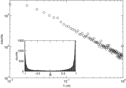
FIG. 2.: Histogram (shown as insert) of the reconstruction order parameter, $m$, at $L=32$ and $K=-3.2$ from a total of $2^{18}$ data points using $\Delta M=0.01$ as bin width. The tails about the peaks at $m=\pm 1$ scale as power laws with exponent $-0.9\pm 0.1$.

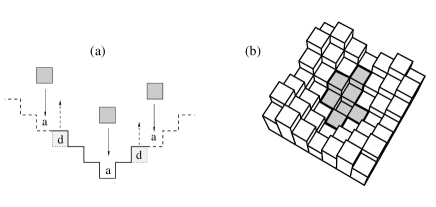
FIG. 3.: (a) One dimensional cross section of the surface near a valley with two loop segments. The sites a (d ) are the only active adsorption (desorption) sites. The domain walls always move upwards during adsorption. (b) A loop of size of $l_{c}$ nucleated at the bottom of the local valley. Gray and white sites have different surface reconstruction parity order.

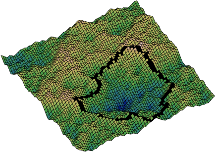
FIG. 4.: A MC surface configuration (at $K=-3.3$ and $L=64$) with a macroscopic loop (the dark line) trapped at a surface ridge line.

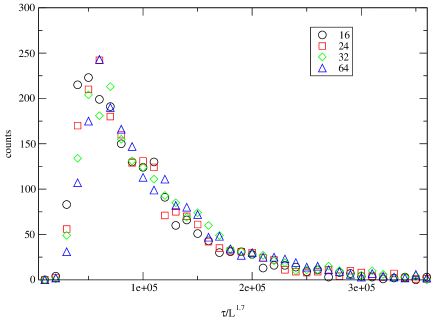
FIG. 5.: Histogram of the decay time of a trapped loop. The data collapses onto a single curve by rescaling time by a factor $L^{1.7}$.

REFERENCES

- [1] The Chemical Physics of Solid Surfaces and Heterogeneous Catalysis, Vol. 7 edited by D. King (Elsevier, Amsterdam, 1994).
- [2] P. Nozières and F. Gallet, J. Phys.(Paris) 48, 353(1987).
- [3] A. Pimpinelli and J. Villain,Physics of Crystal Growth (Cambridge University Press, 1997).
- [4] M. Kardar, G. Parisi, and Y.C. Zhang, Phys. Rev. Lett. 56, 889 (1986); T. Halpin-Healy and Y.C. Zhang, Phys. Rep. 254, 215 (1995).
- [5] M. den Nijs, Phys. Rev. B 46, 10386(1992).
- [6] M. den Nijs, chapter 4 in ref.1.
- [7] B. Drossel, and M. Kardar, cond-mat/0002032.
- [8] M. Kotrla, and M. Predota, Europhys. Lett. 39, 251 (1997); M. Kotrla, F. Slanina and M. Predota, Phys. Rev. B 58, 10003 (1998).
- [9] J.D. Noh, H. Park, and M. den Nijs, Phys. Rev. Lett., in press.
- [10] M. den Nijs, J. Phys. A 18, L549 (1985).
- [11] J.M. Kim and J.M . Kosterlitz, Phys. Rev. Lett.62, 2289 (1989).
- [12] J.G. Amar and F. Family, Phys. Rev. Lett.64, 543 (1990), ibid. 64, 2334 (1990); J. Krug and H. Spohn ibid. 64, 2332 (1990); J. Kim, T. Ala-Nissila and J.M. Kosterlitz ibid. 64, 2333 (1990).
- [13] C.S. Chin and M. den Nijs, Phys. Rev. E. 59 , 2633-2641 (1999).
- [14] K. Binder, and D. W. Heermann, Monte Carlo Simulation in Statistical Physics (Springer-Verlag, Heidelberg, 1997).
- [15] C.S. Chin, in progress.