On the reliability of mean-field methods in polymer statistical mechanics

Abstract

The reliability of the mean-field approach to polymer statistical mechanics is investigated by comparing results from a recently developed lattice mean-field theory (LMFT) method to statistically exact results from two independent numerical Monte Carlo simulations for the problems of a polymer chain moving in a spherical cavity and a polymer chain partitioning between two confining spheres of different radii. It is shown that in some cases the agreement between the LMFT and the simulation results is excellent, while in others, such as the case of strongly fluctuating monomer repulsion fields, the LMFT results agree with the simulations only qualitatively. Various approximations of the LMFT method are systematically estimated, and the quantitative discrepancy between the two sets of results is explained with the diminished accuracy of the saddle-point approximation, implicit in the mean-field method, in the case of strongly fluctuating fields.

1 Introduction

Recently, there has been renewed interest [1, 2, 3, 4] in the venerable problem of polymer partitioning [5, 6]. This phenomenon is of interest both from a theoretical as well as a practical perspective. Macromolecular separation techniques, such as size exclusion chromatography, gel electrophoresis, filtration, membrane separation, etc. [7] all have their basis in polymer partitioning—the property of macromolecular chains to distribute themselves in a network of random obstacles according to their molecular weight/length or electric charge. These phenomena are also of fundamental interest for understanding the properties of macromolecules and complex fluids.

In some recent work [8, 4] we developed a lattice field theory approach to the statistical mechanics of polymers in solution. This approach relied on several approximations: the treatment was at the mean-field level, which amounts to a saddle-point approximation to the system’s partition function; also the problem was treated on a lattice, converting a continuous three dimensional (3D) problem to a discrete, finite matrix problem, and, finally, the polymer chain was assumed to be long enough so that it was approximated as a continuous object, ignoring the discrete character of the building monomers.

The goal of this paper is to investigate the range of validity of these approximations. In order to do so we need to make a comparison with an exact solution of the problem, which can be obtained in the case of neutral polymers by numerical Monte Carlo simulations. We are mostly interested in the reliability of the mean-field approach and its implicit saddle-point approximation, and the cases in which it can be applied with a high level of accuracy.

In Section 2 of the paper we generalize our previous treatment to the case of a soft short-range interaction potential between the monomers in the polymer chain, which is needed for the direct comparison with the simulation results. In this section we also discuss the other two types of errors, namely the lattice discretization error and the error due to the approximation of the chain as a continuous object—we shall call it the “chain continuity error”—and the need for their elimination in order to estimate the reliability of the mean-field approach per se. In Section 3 we show how the chain continuity error can be eliminated by a transfer matrix representation of the partition function, and discuss the effects of this error for the problem of a polymer chain in a spherical cavity. Here also we show how the transfer matrix approach can be extended to the more general case of a 3D lattice. In Section 4 we present results for the monomer distribution of a polymer chain in a sphere from the transfer matrix approach and compare them with those for the case of a continuous chain, and with the exact simulation results, showing a good agreement between the three approaches. In Section 5 we describe the procedures used in two different numerical simulation methods, and present the results obtained by these two independent methods compared with the results obtained by the mean-field method using the transfer matrix approach, for the problem of a polymer chain confined to move within the region of two connected spheres. The results show that for certain range of parameters there is a substantial deviation between the mean-field approach and the simulations, which is clearly due to the large fluctuations in the monomer repulsion field. We are presently working on a method that would allow us to overcome this problem by applying the mean-field approach separately in different regions where it is accurate, and “welding” the results for the polymer partition function of the separate regions to obtain an accurate description of the more complicated physical situation. In Section 6 we outline possible applications of the methods and conclude.

2 A strategy for studying the accuracy of the mean-field approximation in polymer problems

In order to study systematically the level of accuracy of the mean-field approach to polymer statistical mechanics introduced in some recent work of the present authors [8, 4], it will be convenient to introduce a slightly generalized Hamiltonian which allows for a soft Yukawa type repulsive potential between the monomers of the polymer chain [9]. In such a model (absent long-range electrostatic interactions, which are not treated in this paper) an essentially exact (up to statistical errors) solution of the statistical mechanics is available via standard Monte Carlo simulation methods, while, as we shall see below, the mean-field Schrödinger approach of [8, 4] can be generalized to such a model, allowing a direct comparison and evaluation of the error incurred by the saddle-point approximation implicit in the mean-field equations.

The partition sum for a Gaussian polymer chain of $M$ monomers with a repulsive Yukawa potential acting between any pair of monomers on the chain and a general exclusion potential $V_{\rm excl}(\vec{r})$ (which can be used to exclude monomers from certain regions of space) can be written

$$Z_{{\rm pol}} = \int\prod_{s}d\vec{x}_{s}e^{-\frac{3}{2a_{p}^{2}}\sum_{s=0}^{M-1}(\vec{x}_{s+1}-\vec{x}_{s})^{2}-\frac{\lambda}{2}\sum_{s,s^{\prime}}V_{\rm Yuk}(\vec{x}_{s}-\vec{x}_{s^{\prime}})-\sum_{s}V_{\rm excl}(\vec{x}_{s})}.$$ (1)

Here $s,s^{\prime}$ are integers labelling the monomer location on the chain and the Yukawa repulsion between two monomers with coordinate separation $\vec{r}$ is

$$V_{\rm Yuk}(\vec{r})=\frac{e^{-|\vec{r}|/\sqrt{\gamma}}}{4\pi\gamma|\vec{r}|}.$$ (2)

The unconventional choice of $\sqrt{\gamma}$ for the range of the potential will simplify the algebra later on (in particular, the attentive reader will recognize that $V_{\rm Yuk}$ is exactly the Green’s function of the differential operator $1-\gamma\Delta$). The partition function in (1) involves a positive Boltzmann measure with short range interactions and is therefore susceptible to a standard Monte Carlo simulation. We have found it convenient to perform the simulation by updating the monomer locations with a heat-bath algorithm for the Gaussian part of the Hamiltonian in (1), followed by a Metropolis accept/reject step to include the effects of the Yukawa and exclusion potentials $V_{\rm Yuk},V_{\rm excl}$ (cf. Section 4 for more details).

In the mean-field approach to polymer equilibrium statistical mechanics developed in our recent work [8, 4], we have generally assumed that the polymer chains are sufficiently long that the discrete sums over the monomer index $s$ in (1) may be replaced by a continuous integral over a dimensionless variable $s$, also running from 0 to $M\equiv$ total number of monomers in the chain. From the point of view of the original model (1) (for which we shall have essentially exact—up to controllable statistical error—results via simulation) this is an approximation, which we have termed the “chain continuity approximation” (to distinguish it from the lattice discretization approximation, for example, in which fields on continuous 3-space are replaced by fields defined on a 3D spatial lattice). In this approximation, (1) becomes a path integral

$$Z_{{\rm pol}}=\int D\vec{x}(s)e^{-\frac{3}{2a_{p}^{2}}\int_{0}^{M}ds\dot{\vec{x}}^{2}(s)-\frac{\lambda}{2}\int d\vec{r}d\vec{r}\,^{\prime}j(\vec{r})V_{\rm Yuk}(\vec{r}-\vec{r}\,^{\prime})j(\vec{r}\,^{\prime})-\int_{0}^{M}dsV_{\rm excl}(\vec{x}(s))},$$ (3)

with

$$j(\vec{r})\equiv\int ds\delta(\vec{r}-\vec{x}(s)),$$ (4)

where we have introduced a line distribution $j(\vec{r})$ with support along the line tracing through the monomers. To establish contact with the models studied in our previous work [8, 4], we linearize the dependence on $j$ by introducing an auxiliary field $\omega$ via a Hubbard-Stratonovich transformation. The path integral (3) then becomes

$$Z_{{\rm pol}}=\int D\vec{x}(s)D\omega(\vec{r})e^{-\frac{3}{2a_{p}^{2}}\int_{0}^{M}ds\dot{\vec{x}}^{2}(s)-\frac{\lambda}{2}\int d\vec{r}\omega(\vec{r})(1-\gamma\Delta)\omega(\vec{r})-i\lambda\int d\vec{r}j(\vec{r})\omega(\vec{r})}.$$ (5)

With the range $\sqrt{\gamma}$ set to zero, we recover the simpler model studied in our earlier mean-field papers [8, 4] for the special case of uncharged polymer chains. Here we have specialized to the case of a single particle potential $V_{\rm excl}$ in (3) which is either zero or $+\infty$, and the sole effect of which is to restrict the fields in the path integral (5) to have support in the region where $V_{\rm excl}=0$. The path integral over $\vec{x}(s)$ can be replaced in the standard way by an equivalent Schrödinger problem for the imaginary time evolution (from 0 to $M$) of a particle of mass 3/$a_{p}^{2}$ in an imaginary potential $i\lambda\omega(\vec{r})$. Thus

$$Z_{\rm{pol}}=\int D\omega(\vec{r})e^{-\frac{\lambda}{2}\int\omega(\vec{r})(1-\gamma\Delta)\omega(\vec{r})}Z_{{\rm Schr}}(\omega),$$ (6)

with

$$Z_{{\rm Schr}}(\omega)\equiv\int D\vec{x}(s)e^{-\frac{3}{2a_{p}^{2}}\int_{0}^{M}ds\dot{\vec{x}}^{2}(s)-i\lambda\int ds\omega(\vec{x}(s))}.$$ (7)

The mean-field approximation to the system (6–7) amounts to rerouting the functional integral over $\omega$ through a complex saddle point at $\omega=-i\omega_{c}$, where $\omega_{c}$ is a real function, at which point the evaluation of the Schrödinger amplitude $Z_{\rm Schr}$ in (7) reduces to a conventional 3D quantum mechanical evolution (in imaginary time) of a system subject to the Hamiltonian

$$H\equiv-\frac{a_{p}^{2}}{6}\Delta+\lambda\omega_{c}(\vec{r}).$$ (8)

The hermitian Hamiltonian (8) has a complete set of normalized eigenfunctions $\Psi_{n}(\vec{r})$ with corresponding eigenvalues $E_{n}$, and the evolution amplitude $Z_{\rm Schr}$ appearing in (7) is just

$$Z_{\rm Schr}=\int d\vec{x}_{0}d\vec{x}_{M}<\vec{x}_{0}|e^{-MH}|\vec{x}_{M}>=\int dx_{0}dx_{M}\sum_{n}\Psi_{n}(x_{0})\Psi_{n}(x_{M})e^{-ME_{n}}.$$ (9)

It has been conventional to assume ground state dominance in evaluating $Z_{\rm Schr}$, but this condition is frequently violated in the systems studied below [3, 4]. In a recent paper, we have presented the general solution [4] which makes no assumption of ground state dominance. Defining $Z_{\rm Schr}\equiv e^{F_{\rm pol}}$, and

$$A_{n}\equiv\int d\vec{r}\Psi_{n}(\vec{r}),$$ (10)

we have

$$F_{\rm pol}=\ln{\sum_{n}A_{n}^{2}e^{-ME_{n}}}.$$ (11)

The saddle point of the functional integral (6) is then found by minimizing the functional

$$F=\frac{\lambda}{2}\int d\vec{r}\omega_{c}(\vec{r})(1-\gamma\Delta)\omega_{c}(\vec{r})+F_{\rm pol}(\omega_{c}).$$ (12)

Varying this functional as in our previous work [4], we obtain:

$$\frac{{\delta}F_{pol}}{\delta\omega_{c}(\vec{r})}=\lambda\rho(\vec{r}),$$ (13)

where

$$\rho(\vec{r})=-\frac{\sum_{n,m}\frac{A_{n}\Psi_{n}A_{m}\Psi_{m}}{E_{n}-E_{m}}\left(e^{-ME_{n}}-e^{-ME_{m}}\right)}{\sum_{n}A_{n}^{2}e^{-ME_{n}}}.$$ (14)

Therefore,

$$\frac{1}{\lambda}\frac{\delta F}{\delta\omega_{c}(\vec{r})}=(1-\gamma\Delta)\omega_{c}(\vec{r})-\rho(\vec{r})=0\,.$$ (15)

Equation (15) implies

$$\omega_{c}(\vec{r})\equiv\hat{\rho}(\vec{r})=\int V_{Yuk}(\vec{r}-\vec{r}\,^{\prime})\rho(\vec{r}\,^{\prime})d\vec{r}\,^{\prime},$$ (16)

so that the saddle-point value of the auxiliary field $\omega(\vec{r})$ can be thought of either as a smeared version of the monomer density $\rho$ or as the total repulsive potential at $\vec{r}$ due to all monomers. We may therefore eliminate the auxiliary field altogether in (8), leading to the following mean-field equation describing the equilibrium properties of the polymer chain:

$$\frac{a_{p}^{2}}{6}\vec{\nabla}^{2}\Psi_{n}(\vec{r})=\lambda\hat{\rho}(\vec{r})\Psi_{n}(\vec{r})-E_{n}\Psi_{n}(\vec{r}).$$ (17)

This equation is a generalization of Eq. (22) in our previous work [4] for the Yukawa type interaction potential between monomers. It is a continuous mean-field nonlinear Schrödinger type equation which in general must be solved numerically by putting the system on a discrete spatial lattice. This introduces (in addition to the errors incurred by making the chain continuous and the saddle-point approximation of (5)) a third source of error in comparing the results with the exact solution (via Monte Carlo) of the original system (1). The determination of the qualitative effects and relative size of all three sources of error in some systems of interest is the primary focus of this paper. In particular, it will be important to understand the size of the chain continuity error and lattice discretization effects in determining the extent to which the mean-field approximation per se fails or succeeds in a specific polymer problem.

3 Discrete vs continuous chains: a transfer matrix approach

In this section we estimate the size of the error incurred by replacing a discrete chain of $M$+1 monomers in (1) by a continuous imaginary-time Schrödinger evolution as in (7). For simplicity, we first study this issue with $\lambda$ = 0 (no intermonomer repulsion) for a polymer chain confined to a spherical region of radius $R$. In this simple case the main qualitative effect of this replacement is to force the monomer density to vanish exactly at the boundary of the sphere, whereas there is a finite average density of monomers at the boundary in the case of the discrete chain [10]. It turns out that a transfer matrix formalism allows a simple analytic description of the discrete chain case, which enables us to derive an explicit formula for the size of this “wall effect”.

Referring to the partition sum (1), introduce a transfer matrix $T(\vec{x},\vec{x}\,^{\prime})$ as follows:

$$T(\vec{x},\vec{x}\,^{\prime})\equiv\Theta_{S}(\vec{x})\Theta_{S}(\vec{x}\,^{\prime})e^{-\alpha(\vec{x}-\vec{x}\,^{\prime})^{2}},\;\;\;\alpha\equiv\frac{3}{2a_{p}^{2}},$$ (18)

where $\Theta_{S}(\vec{x})$ is the Heaviside theta-function with support inside the sphere of radius $R$. Viewing the transfer-matrix as a linear operator kernel, the partition function (1) can then be written simply as:

$$Z_{\rm pol}=\int d\vec{x}_{0}d\vec{x}_{M}T^{M}(\vec{x}_{0},\vec{x}_{M}).$$ (19)

On the other hand, we can define a Hamiltonian $H_{\rm d}$ for the discrete chain by the usual connection, $T=e^{-H_{\rm d}}$, so that

$$Z_{\rm pol}=\int d\vec{x}_{0}d\vec{x}_{M}<\vec{x}_{0}|e^{-MH_{\rm d}}|\vec{x}_{M}>.$$ (20)

Of course, the operator $H$ in (8) and (9) and $H_{\rm d}$ differ, and it is precisely this discrepancy which we have referred to previously as the “chain continuity error”. Note that the integrals over initial and final monomer locations in Eqs. (9) and (20) (corresponding to free boundary conditions for an open polymer chain) restrict us to s-wave (spherically symmetric) eigenfunctions of both $H$ and $H_{\rm d}$. In the case of the Schrödinger operator $H$, these eigenfunctions are the familiar spherical Bessel functions and the corresponding eigenvalues are related in the usual way to the zeroes of these radial functions [as $\Psi_{n}(r{=}R)=0$ in the continuous chain approximation]. For the discrete chain operator, we must diagonalize the integral kernel $T$ in (18). The eigenvalues $\varepsilon_{n}$ of $T$ are related to the eigenvalues $E_{n}$ of $H_{\rm d}$ by $\varepsilon_{n}=e^{-E_{n}}$, while the eigenfunctions of $T$ and $H_{\rm d}$ are the same. Restricting ourselves to spherically symmetric eigenfunctions, we need to solve the linear integral equation

$$\int_{r^{\prime}<R}e^{-\alpha|\vec{r}-\vec{r}\,^{\prime}|^{2}}\psi(\vec{r}\,^{\prime})d\vec{r}\,^{\prime}=\varepsilon\psi(\vec{r}),$$ (21)

which reduces after integration over angles to the one dimensional (1D) integral equation

$$\frac{\pi}{\alpha}\int_{0}^{R}dr^{\prime}\left(e^{-\alpha(r-r^{\prime})^{2}}-e^{-\alpha(r+r^{\prime})^{2}}\right)f(r^{\prime})=\varepsilon f(r),$$ (22)

where $f(r)\equiv r\psi(r)$. This equation can easily be solved by discretization and numerical diagonalization, whence one finds the “wall effect” previously mentioned, namely $f(R)\neq 0$ (this effect is also visible in explicit simulations, cf. Section 4). We can estimate the size of the effect in the limit $a_{p}\ll R$ (which implies $\alpha R^{2}\gg 1$ and the negligibility of the second exponential for $r\simeq R$ in (22)) as follows. To leading order in $a_{p}/R$, the radial transfer matrix in (22)) is

$$\int e^{-\alpha(r-r^{\prime})^{2}}f(r^{\prime})dr^{\prime}\simeq\sqrt{\frac{\pi}{\alpha}}\left(1+\frac{1}{4\alpha}\frac{d^{2}}{dr^{2}}\right)f(r).$$ (23)

The ground state corresponds to the eigenvalue $-\left(\frac{\pi}{R}\right)^{2}$ of $\frac{d^{2}}{dr^{2}}$, so in this limit the $\varepsilon$ eigenvalue of the ground state is $\varepsilon_{0}\approx\left(\frac{\pi}{\alpha}\right)^{3/2}\left(1-\frac{\pi^{2}}{4\alpha R^{2}}\right)$. Next, writing $f(r)\simeq\delta+\sin\left(\pi\frac{r}{R}\right),\;\;r\simeq R$, and substituting this ansatz into (23) at $r=R$, we find

$$\int e^{-\alpha(r^{\prime}-R)^{2}}\left(\delta+\sin\left(\pi\frac{r^{\prime}}{R}\right)\right)dr^{\prime}\simeq\frac{\varepsilon\alpha}{\pi}\delta.$$ (24)

The radial integral can be evaluated in the given approximation by linearizing the sine function near $r=R$, $\sin\left(\frac{\pi r^{\prime}}{R}\right)\approx\frac{\pi}{R}(R-r^{\prime})$, whereupon we find

$$\frac{\varepsilon\alpha}{\pi}\delta\simeq\frac{1}{2}\sqrt{\frac{\pi}{\alpha}}\delta+\frac{1}{2\alpha}\frac{\pi}{R}.$$ (25)

Substituting the value $\varepsilon_{0}$ found above for the ground state, we find the size of the wall effect to leading order in $1/\alpha R^{2}$ to be

$$\delta\simeq\sqrt{\frac{\pi}{\alpha}}\frac{1}{R}=\sqrt{\frac{2\pi}{3}}\frac{a_{p}}{R}.$$ (26)

It should be noted that this estimate is conditioned on $f(r)$ being approximated by $\sin\left(\pi\frac{r}{R}\right)$, that is, $f(r)$ is normalized to be approximately unity at $r=R/2$. In the next section we shall present numerical results for the single sphere system confirming this analytic estimate.

For more general problems in three dimensions, lacking spherical symmetry (such as the two sphere situation studied in Section 5) it is still possible to diagonalize the transfer matrix, in this case by going to a discrete spatial lattice with lattice spacing $a$. Then the transfer matrix (in this case, truly a finite dimensional matrix!) becomes

$$T_{\vec{n}\vec{m}}=e^{-\frac{3a^{2}}{2a_{p}^{2}}|\vec{n}-\vec{m}|^{2}-\frac{1}{2}(V_{\vec{n}}+V_{\vec{m}})},$$ (27)

where $V_{\vec{n}}$ is the value of the single-particle potential $V_{\rm excl}$ in (1) at the lattice point $\vec{n}$ (recall that we are still taking $\lambda=0$ in (1)). Although in principle a non-sparse matrix, we have found it perfectly adequate to cutoff the matrix elements of (27) for $|\vec{n}-\vec{m}|>6$, whereupon the remaining relatively sparse matrix can be diagonalized by standard Lanczos techniques. The results of calculations employing this transfer matrix, and therefore eliminating the chain continuity error in comparisons with the Monte Carlo simulations of (1), are given in the following two sections.

If the intermonomer repulsion $V_{\rm Yuk}$ is present then the transfer matrix formalism can still be employed to estimate the chain continuity error, but only in the context of the mean-field approximation discussed in the previous section. After introducing the auxiliary field $\omega$ and going to the complex saddle point at $\omega=-i\omega_{c}$, we can reinstate a discrete chain by using the transfer matrix (27) with $V_{\vec{n}}$ taken equal to the value of $V_{\rm excl}+\lambda\omega_{c}$ at the lattice point $\vec{n}$, where $\omega_{c}$ is again given by the formula (16) and $\rho(\vec{r})$ by (14), with slightly different coefficients $A_{d,n}$ defined as

$$A_{d,n}\equiv\int d\vec{r}e^{-(1/2)V(\vec{r})}\Psi_{n}(\vec{r}).$$ (28)

4 Comparison of transfer matrix and simulation results for a polymer chain in a spherical cavity

In this section we consider a polymer chain of 100 monomers, restricted to move within the volume of a spherical cavity. We have chosen the Kuhn length to be unity and a sphere radius equal to ten. First, we discretize the integral equation (22) (neglecting the second exponential) on a fine 1D lattice, thus converting it into a standard matrix eigenvalue problem, which we solve to a high precision. The solution involves only spherically symmetric s-waves. In Fig. 1 we plot the function $f(r)$ defined in the previous section by Eq. (22), which clearly exhibits the “wall effect” discussed earlier—it has a finite value at the edge of the sphere. The value $f(R)$ in Fig. 1 is 0.139, which is close to the value calculated from Eq. (26) for the given set of parameters, $\delta\approx 0.145$.

Then we apply the Lanczos procedure described in our earlier work [8, 4] to obtain the eigenvalues and eigenvectors of the transfer matrix (18), and therefore the monomer density. The matrix is discretized on a cubic lattice of 44 points on each side, with lattice spacing $a=a_{p}/2$, in which the spherical cavity is embedded. The resulting radial monomer density is plotted on Fig. 2, where it is compared with the exact result from a Monte Carlo heat bath simulation (described in the next section), the 1D transfer matrix result of Eq. (22), and the result from the Schrödinger equation approach, Eq. (17), for $\lambda$ = 0. We see that the exact simulation result practically coincides with the results obtained via the transfer matrix approach. In these cases the monomer density has a finite value at the wall. In the case of the Schrödinger approach, where the chain continuity error is present, the radial monomer density vanishes at the wall, as expected.

Since above we have considered a Gaussian chain without excluded volume effects, there is no saddle-point error in this calculation; we are left with the lattice discretization and chain continuity errors. From a comparison between the 1D and 3D transfer matrix results in Fig. 2, it is clear that in this case the lattice discretization error is practically non-existent, as the results from the fine 1D lattice virtually coincide with these from the rough 3D lattice. From the same figure it is also clear that the major error in this case of no excluded volume interactions is the chain continuity error, which is also insignificant.

Figure 1: The radial function $f(r)$ exhibiting a finite value at the edge of the sphere.

Figure 2: A comparison between results from the Monte Carlo heat bath simulation (exact), the transfer matrix approach, and the Schrödinger equation approach, for the radial monomer density $P(r)$ of a Gaussian polymer chain of 100 monomers without excluded volume interactions with a Kuhn length unity in a spherical cavity of radius ten. (The error bars of the simulation curve are within the size of the symbols used to mark it.) The “wall effect” is less apparent in this figure as we are plotting the monomer density (roughly speaking, the square of $f(r)$ in Fig. 1).

In Fig. 3 we show an analogous plot of the radial monomer density with all parameters the same as in Fig. 2 but with excluded volume interactions present with $\lambda=0.0012$. It is clear that in this case there is an error due to the saddle-point approximation, leading to a deviation between the transfer matrix and the simulation result. Here, again, the “wall effect” is present in the simulation and the transfer matrix density, while the density resulting from the Schrödinger equation approach vanishes at the wall.

Figure 3: A comparison between results from the Monte Carlo heat bath simulation (exact), the transfer matrix approach, and the Schrödinger equation approach, for the radial monomer density $P(r)$ of a polymer chain of 100 monomers with excluded volume interactions with $\lambda=0.0012$. The Kuhn length is unity and the spherical cavity has a radius of ten. (The error bars of the simulation curve are within the size of the symbols used to mark it.)

5 Comparison between lattice field theory and simulation results for a polymer chain partitioned between two connected spherical cavities of different radii

The simulation of the system (1) by Monte Carlo techniques is readily accomplished given the absence of long-range forces. We have chosen to perform the simulation by generating new polymer configurations using a heat-bath algorithm on the Gaussian part of the Boltzmann measure $e^{-\frac{3}{2a_{p}^{2}}\sum_{s=0}^{M-1}(\vec{x}_{s+1}-\vec{x}_{s})^{2}}$, rejecting the obtained configuration if it is forbidden by the exclusion potential $V_{\rm excl}$ (here assumed to be either zero or $\infty$), and then correcting for the remaining Yukawa potential with a Metropolis accept/reject step. Specifically, the algorithm employed is as follows:

1. First, a monomer location $i$ is chosen at random (i.e. an integer between 0 and $M-1$) and a new location $\vec{x}_{i}$ generated according to the weight

   $$e^{-\frac{3}{2a_{p}^{2}}\sum_{s=0}^{M-1}(\vec{x}_{s+1}-\vec{x}_{s})^{2}}\propto e^{-3(\vec{x}_{i}-\vec{d}_{i})^{2}/a_{p}^{2}},$$ (29)

   where $\vec{d}_{i}\equiv\frac{1}{2}(\vec{x}_{i-1}+\vec{x}_{i+1})$.

2. If the new location $\vec{x}_{i}$ is outside the allowed region (as determined by the exclusion potential) it is rejected and a new $\vec{x}_{i}$ found by the preceding algorithm.

3. The Yukawa part of the Hamiltonian, $S_{\rm Yuk}\equiv\frac{\lambda}{2}\sum_{s,s^{\prime}}V_{\rm Yuk}(\vec{x}_{s}-\vec{x}_{s^{\prime}})$ is used to accept/reject the new configuration (Metropolis update), with Yukawa Hamiltonian $S_{\rm Yuk}^{\prime}$ as follows:
   (a) if $S_{\rm Yuk}^{\prime}<S_{\rm Yuk}$, the new configuration is accepted without further ado,
   (b) if $S_{\rm Yuk}^{\prime}>S_{\rm Yuk}$, the new configuration is accepted with probability $e^{-S_{\rm Yuk}^{\prime}+S_{\rm Yuk}}$. If it is rejected, the monomer is left unmoved.

In order to obtain confidence in our results, we have performed a second dynamic Monte Carlo simulation based on the kink-jump technique developed by Baumgärtner and Binder [11]. In this method the polymer chain is treated as a “pearl-necklace” in which every two consecutive monomers are connected by a rigid rod of length $l$. Monomers are modeled as hard spheres, whose radius $r_{m}$ can be adjusted to describe the strength of the excluded volume interaction. Initially the chain is placed in the allowed region with the positions of its monomers chosen randomly. Then the chain dynamics is evolved by the kink-jump technique: at each time step a monomer is picked, say the $n$th one, and then it is rotated around the axis connecting the $(n-1)$th and the $(n+1)$th monomers at a random angle. If an end monomer is chosen, it is moved to a new random position keeping the rod length between it and the monomer to which it is connected fixed. The move is accepted if the monomers do not overlap and stay within the allowed region.

We apply these two simulations methods to a polymer chain confined to move within two connected spheres of different radii. In relative units, we choose the big sphere to have a radius $R_{1}$ equal to unity, the small one has a radius $R_{2}=0.8$, the Kuhn length is chosen to be $a_{p}=0.2$, and the spheres are embedded in each other with the distance between their centers fixed at 1.7. This system is schematically shown in Fig. 4.

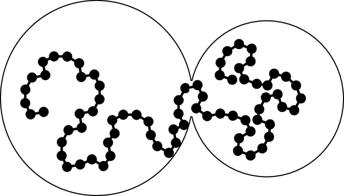
Figure 4: A polymer chain confined to move within two connected spheres.

We have calculated the polymer partition coefficient $K$, defined as the ratio of the average number of monomers in the big and small spheres respectively, $K\equiv\left<M_{1}\right>/\left<M_{2}\right>$, where the total number of monomers is $M=\left<M_{1}\right>+\left<M_{2}\right>$, for varying $M$. First, in Fig. 5 we show the simulation results for the case of a non-interacting chain. These results are compared with lattice field calculations using the transfer matrix and the Schrödinger equation approaches. As in the case described in the previous section, we see that the agreement between all the different approaches is very good for the case of zero interaction between the monomers, which confirms once again that the chain continuity and lattice discretization errors are small. In this figure the result from the Schrödinger equation approach appears to be closer to the statistically exact simulation result than the transfer matrix result, probably due to a coincidental cancellation of errors. Here, and in the next two figures, we observe that in the case of longer chains the transfer matrix approach produces a partition coefficient which is systematically smaller than the one resulting from the simulations.

Figure 5: $\ln{K}$ vs $M$ for the case of a Gaussian chain with no excluded volume interactions. The simulation results are seen to agree with the lattice field calculations.

In Fig. 6 we show results for $\ln{K}$ from the simulations for the interacting chain with $\lambda_{1}=0.0012$ and $\gamma=a_{p}^{2}$ for system (1), which is matched to a monomer radius $r_{m,1}=0.025$ in the kink-jump technique. These results are also compared to the results obtained via the transfer matrix lattice field calculation for the same parameters used in the Monte Carlo heat bath/metropolis calculation. In this calculation the two-sphere system is modeled on a discrete cubic lattice of 44 points on each side with lattice spacing $a=0.1$ as described in [3, 4]. In our previous work [3] we have shown that the size of the aperture connecting the two spheres plays an important role in determining the value of the partition coefficient $K$. However, when the system shown in Fig. 4 is modeled on a lattice, lattice artifacts prevent us from obtaining the exact same aperture size, as in the continuous case. Therefore, the aperture size on the lattice is adjusted to be as close as possible to the one in the continuous case shown in Fig. 4.

In our previous work [8] we have shown that the excluded volume parameter $\lambda$ can be connected to the monomer radius via the second virial coefficient, leading to the expectation that

$$\lambda\approx{\rm const}\times r_{m}^{3}.$$ (30)

From the parameters of the calculation whose results are presented in Fig. 6 we calculate ${\rm const}$ and use it to calculate a second excluded volume parameter, $\lambda_{2}=0.0033$, corresponding to the monomer radius $r_{m}=0.035$, and then we perform simulations for the two new sets of parameters by the heat bath/metropolis method and the kink-jump technique, and present the results in Fig. 7. The good agreement between this second set of simulations confirms formula (30). We have also performed the mean-field transfer matrix calculations for this new $\lambda$, and have plotted the results for comparison in the same figure.

Figure 6: $\ln{K}$ vs $M$ for $\lambda=0.0012$, which is matched to $r_{m}=0.025$. The mean-field transfer matrix results for the same $\lambda$ are seen to disagree substantially with the statistically exact results, although in both curves there is a maximum with a turnover.

Figure 7: $\ln{K}$ vs $M$ for $\lambda=0.0032928$, corresponding to $r_{m}=0.035$ in the kink-jump simulation technique. The mean-field transfer matrix results for the same $\lambda$ are seen to disagree with the simulation results, although both curves possess the same generic features.

From Figs. 6 and 7 we observe that $\ln{K}$ increases almost linearly with $M$ for small $M$, then goes through a turnover, and at large $M$ decreases to a limiting value determined by the ratio of the volumes of the two spheres. From the simulations we observe that, as is to be expected, the turnover occurs when the end-to-end distance of the polymer chain becomes comparable to the diameter of the larger sphere. Both Figs. 6 and 7 show that although the mean-field results show the same generic behavior, they deviate substantially from the exact simulation results. Since we have eliminated the chain continuity error by using the transfer matrix approach, and we have already seen that the lattice discretization error in these calculations is relatively small, we conclude that the quantitative discrepancy between the statistically exact simulation results and the mean-field results is due mainly to the saddle-point approximation implicit in the mean-field approach. Also, it should be noted that in these cases the mean-field results from the Schrödinger equation approach (not shown in the figures) are very close to the transfer matrix results, leading to the conclusion that the chain continuity error is small in the case of excluded volume interactions too.

The results show that the error is larger in the cases of shorter chains, while in the cases of longer chains it is relatively small. This can be explained with the help of the following observation made in the course of the simulations: the shorter chains tend to be localized entirely in one sphere or the other (thus achieving a higher conformational entropy), and only make infrequent jumps between the two spheres. This creates a highly fluctuating monomer repulsion field and renders the saddle-point approximation less reliable. In the case of a long chain, monomer repulsion competes with the free energy gain due to the higher conformational entropy, and the chain tends to stretch between the two spheres, occupying both of them simultaneously for most of the time. In that case the monomer repulsion field exhibits smaller fluctuations and the saddle-point approximation is expected to be better. To illustrate this point, in Fig. 8 we show a plot of the number of monomers in the bigger sphere, $M_{1}$, as a function of the number of simulation sweeps, for two different cases, $M=500$ and $M=100$, for the parameters corresponding to Fig. 7. It is seen that the relative fluctuations in $M_{1}$ are much larger for the smaller $M$.

Figure 8: The number of monomers in the bigger sphere, $M_{1}$, as a function of the number of simulation sweeps $t$ for $M=100$ (left plot) and $M=500$ (right plot), for the parameters corresponding to Fig. 7.

It is also important to point out that what we actually measure in the simulations is the average number of monomers in the big sphere, $\left<M_{1}\right>$, and the partition coefficient $K$ computed from it is very sensitive to small errors in $\left<M_{1}\right>$, as $\left<M_{1}\right>$ and $\left<M_{2}\right>$ are constrained to add to $M$, hence a small error in $\left<M_{1}\right>$ will automatically be reflected in $\left<M_{2}\right>$ with an opposite sign, thus amplifying the error in the ratio $K$, especially when $\left<M_{1}\right>$ is much bigger than $\left<M_{2}\right>$, as in the calculations presented here. The actual error between the mean-field calculations and the simulations is, in fact, much smaller than one would infer from Figs. 6 and 7. To illustrate this point, in Fig. 9 we plot the results for $\left<M_{1}\right>$ and $\left<M_{2}\right>$ as a function of $M$ from the calculations corresponding to the $\ln{K}$ plot in Fig. 7.

Figure 9: The average number of monomers in the bigger and smaller spheres, $\left<M_{1}\right>$ (left plot) and $\left<M_{2}\right>$ (right plot), respectively, as a function of the total number of monomers, $M$, for the parameters corresponding to Fig. 7.

6 Conclusions

The main focus of this work has been investigation of the validity and reliability of mean-field methods in polymer statistical mechanics by systematic elimination and estimation of all errors inherent to the lattice field theory approach developed in our earlier work [8, 4], apart from the saddle-point approximation implicit in the mean-field method. To be able to evaluate these errors we have compared the lattice field theory results to the statistically exact results from two independent Monte Carlo simulations, namely, a heat bath/metropolis computation and a computation based on the kink-jump simulation technique. In the case of no excluded volume interactions, computation of the radial monomer density of a polymer chain constrained to move within a spherical cavity, and of the partition coefficient of a chain restricted to move within two connected spheres, shows that “chain continuity” and “lattice discretization errors” are relatively small. On the other hand, including short-range pair-wise interactions in the Hamiltonian and subsequent mean-field treatment of these via the saddle-point approximation leads to a larger quantitative error in the partition coefficient for problems of certain geometry, as is shown by a comparison with the exact simulation results.

This error is larger for shorter chains, and diminishes for long chains. It has been attributed to the strongly fluctuating monomer repulsion field in the case of short chains, as revealed by the simulations: the short chains preferentially localize entirely in one sphere or the other (thus attaining a higher conformational entropy), making infrequent jumps between the two spheres, which leads to a strongly fluctuating repulsion field felt by each monomer in the chain, and diminishes the validity of the saddle-point approximation, an approximation which assumes smoothly varying fields. In the case of long chains, the large number of monomers leads to a very strong repulsion, overwhelming the gain in conformational entropy which would have been achieved had the whole chain been localized in one of the two spheres, hence the chain stretches into both spheres in its most likely configuration, creating a smoother interaction field felt by the individual monomers. Thus, in this case the saddle-point approximation is expected to be good, and indeed, the mean-field and the simulation results show good agreement.

The calculations presented in this paper suggest that the mean-field approach works very well for problems of polymers moving easily in an open region, but is not very accurate in situations where the polymers are forced to move between several such regions connected only by narrow conduits leading to large fluctuations in the monomer density field. Fortunately, in certain cases it turns out to be possible to “weld” the mean-field results for the polymer partition function in separate open regions into an accurate description of the more complicated situation, so that the saddle-point approximation is only involved where it is accurate. In this way we have been able to reproduce the simulation results of Figs. 6 and 7 for $\ln{K}$. A detailed description of this technique will be presented in a forthcoming publication.

Acknowledgment: This work was supported by the National Science Foundation Grant CHE-9633561. Some of the computations presented were performed at the University of Pittsburgh’s Center for Molecular and Materials Simulation. The work of A.D. was supported in part by NSF grant 97-22097.

References

- [1] L. Liu, P. Li and S.A. Asher, Nature 397, 141 (1999); L. Liu, P. Li and S.A. Asher, J. Am. Chem. Soc. 121, 4040 (1999).
- [2] S.-S. Chern and R.D. Coalson, J. Chem. Phys. 111, 1778 (1999).
- [3] S. Tsonchev and R.D. Coalson, submitted for publication.
- [4] S. Tsonchev, R.D. Coalson and A. Duncan, Phys. Rev. E, in press.
- [5] E.F. Casassa, Polymer Lett. 5, 773 (1967); E.F. Casassa and Y. Tagami, Macromolecules 2, 14 (1967).
- [6] M. Muthukumar and A. Baumgärtner, Macromolecules 22, 1937 (1989).
- [7] D. Rodbard and A. Chrambach, Proc. Nat. Acad. Sci. USA 65, 970 (1970); G. Guillot, L. Leger and F. Rondelez, Macromolecules 18, 2531 (1985).
- [8] S. Tsonchev, R.D. Coalson and A. Duncan, Phys. Rev. E 60, 4257 (1999).
- [9] R.D. Coalson, A.M. Walsh, A. Duncan, and N. Ben-Tal, J. Chem. Phys. 102, 4584 (1995).
- [10] A.Y. Grosberg and A.R. Khokhlov, Statistical Physics of Macromolecules (AIP Press, New York, 1994), p. 46.
- [11] A. Baumgärtner and K. Binder, J. Chem. Phys. 71, 2541 (1979).