Imaging the Phase of an Evolving Bose-Einstein Condensate Wavefunction

Abstract

We demonstrate a spatially resolved autocorrelation measurement with a Bose-Einstein condensate (BEC) and measure the evolution of the spatial profile of its quantum mechanical phase. Upon release of the BEC from the magnetic trap, its phase develops a form that we measure to be quadratic in the spatial coordinate. Our experiments also reveal the effects of the repulsive interaction between two overlapping BEC wavepackets and we measure the small momentum they impart to each other.

A trapped Bose-Einstein condensate [1] has unique value as a source for atom lasers [2] and matter-wave interferometry [3] because its atoms occupy the same quantum state, with uniform spatial phase. However, when released from the trapping potential, a BEC with repulsive atom-atom interactions expands, developing a non-uniform phase profile. Understanding this phase evolution will be important for applications of coherent matter waves. We have developed a new interferometric technique using spatially resolved autocorrelation to measure the functional form and time evolution of the phase of a BEC wavepacket expanding under the influence of its mean field repulsion.

In 1997, the coherence of weakly interacting BECs was demonstrated by releasing two spatially separated condensates and observing their interference [4]. Subsequent experiments have further investigated condensate coherence properties. One [5] used velocity-resolved Bragg diffraction [6] to probe the momentum spectrum of trapped and released BECs. A complementary experiment [7] that used matter-wave interferometry can be interpreted as a measurement of the spatial correlation function, whose Fourier transform is the momentum spectrum. These experiments showed that a trapped condensate has a uniform phase, and a released condensate develops a non-uniform phase profile. (Recently the influence of non-zero temperature on coherence properties was also investigated [8]). The experiments reported in this Letter combine spatial resolution and interferometry to measure the functional form of the time-dependent phase profile of a released condensate. We also make the first measurement of the velocity imparted to two equal BEC wavepackets from their mutual mean-field repulsion [9].

We perform our experiments with a condensate of $1.8(4)\times 10^{6}$ [10] sodium atoms in the $3S_{1/2}$, $F=1$, $m_{F}=-1$ state. The sample has no discernable non-condensed (i.e. thermal) component. The condensate is prepared following the method of Ref. [6] and is held in a magnetic trap with trapping frequencies $\omega_{x}=\sqrt{2}\omega_{y}=2\omega_{z}=2\pi\times$27 Hz. Using a scattering length of $a=2.8$ nm, the calculated Thomas-Fermi diameters [11] are 47 $\mu$m, 66 $\mu$m, and 94 $\mu$m, respectively.

We release the BEC from the magnetic trap and it expands, driven mostly by the mean-field repulsion of the atoms. This expansion implies the development of a nonuniform spatial phase profile (recall that the velocity field is proportional to the gradient of the quantum phase). After an expansion time $T_{0}$, we probe the phase profile with matter-wave Bragg interferometry [12, 13, 14]. Our interferometer splits the BEC into two wavepackets and recombines them with a chosen overlap, producing interference fringes, which we measure with absorption imaging [15]. From the dependence of the fringe spacing on the overlap, we extract the phase profile of the wavepackets.

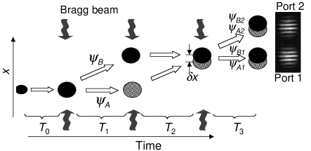
FIG. 1.: Space-time diagram of the experiment. Three optically induced Bragg-diffraction pulses form the interferometer. The condensate is released for a time $T_{0}$ before the first Bragg pulse. The centers of $\psi_{{A}}$ and $\psi_{{B}}$ are separated by $\delta x$ at the time of the third Bragg pulse, which splits them into $\psi_{{A1}}$, $\psi_{{B1}}$, and $\psi_{{A2}}$, $\psi_{{B2}}$. Before imaging the atoms, we allow the output ports to separate for a time $T_{3}\approx 2$ ms. The image shows the output ports when $T_{0}$ = 3 ms, $T_{1}$ = 1 ms, and $T_{2}$ = 1.3 ms.

Our atom interferometer [14] consists of three optically-induced Bragg-diffraction pulses applied successively in time (Fig. 1). Each pulse consists of two counter-propagating laser beams whose frequencies differ by 100 kHz. They are detuned by about $-2$ GHz from atomic resonance ($\lambda=2\pi/k=589$ nm) so that spontaneous emission is negligible. The first pulse has a duration of 6 $\mu$s and intensity sufficient to provide a $\pi/2$ pulse, which coherently splits the BEC into two wavepackets, $\psi_{{A}}$ and $\psi_{{B}}$. The wavepackets have about the same number of atoms and only differ in their momenta: $p=0$ and $p=2\hbar k$. At a time $T_{1}=1$ ms after the first Bragg pulse, the two wavepackets are completely separated and a second Bragg pulse (a $\pi$ pulse) of 12 $\mu$s duration transfers $\psi_{{B}}$ to a state with $p\approx 0$ and $\psi_{{A}}$ to $p\approx 2\hbar k$ [16]. After a variable time $T_{2}$ the wavepackets partially overlap again and we apply a third pulse, of 6 $\mu$s duration (a $\pi/2$ pulse). This last pulse splits each wavepacket into the two momentum states. The interference of the overlapping wavepackets in each of the two momentum states allows the determination of the local phase difference between them. By changing the time $T_{2}$ we vary $\delta x=x_{A}-x_{B}$, the separation of $\psi_{{A}}$ and $\psi_{{B}}$ at the time of the final Bragg pulse. The set of data at different $\delta x$ constitutes a new type of spatial autocorrelation measurement that is similar to the “FROG” technique [17] used to measure the complete field of ultrafast laser pulses. From these measurements we obtain the phase profile of the wavepackets in the $x$ direction.

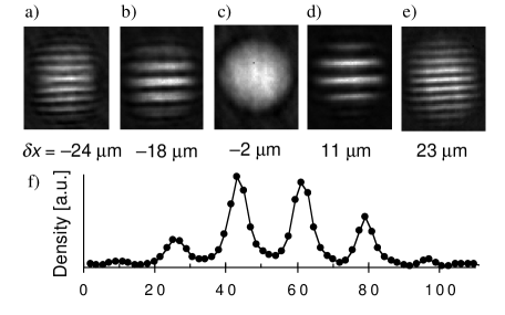
FIG. 2.: (a-e) One of the two output ports of the interferometer with $T_{0}$ = 4 ms and $\delta x$ as indicated. (f) A plot of the density along the $x$ direction of (d).

Figure 2a-e shows one interferometer output port for different $\delta x$ (different $T_{2}$) after an expansion time $T_{0}$ = 4 ms. In general, we observe straight, evenly spaced fringes (although for small $T_{0}$ and $T_{2}$ the fringes may be somewhat curved). There is a value of $\delta x=x_{0}\neq 0$ where we observe no fringes (Fig. 2c) and the fringe spacing decreases as $|\delta x-x_{0}|$ increases. Figure 2f, a cut through Fig. 2d, shows the high-contrast fringes [18]. Our data analysis uses the average fringe period $d$, obtained from plots like Fig. 2f.

The fringes come from two different effects: the interference of two wavepackets with quadratic phase profile, and a relative velocity between the wavepackets’ centers. The data can be understood by calculating the fringe spacing along $x$ at output port 1 [19]. We assume that the phase $\phi$ of the wavefunction $f{\rm e}^{i\phi}$ can be written as $\phi=\frac{\alpha}{2}x^{2}+\beta x$. The equal spacing of the fringes implies, as predicted in the Thomas-Fermi limit [20], that $\phi$ has no significant higher-order terms [21]. The curvature coefficient $\alpha$ describes the mean-field expansion of the wavepackets and $\beta$ describes a relative repulsion velocity. The velocity arises because the wavepackets experience a repulsive push as they first separate and again as they recombine. The density at port 1 (see Fig. 1) just after the final interferometer pulse is the interference pattern $|{\psi_{A1}+\psi_{B1}}|^{2}$ of the wavepackets $\psi_{{A1}}$ and $\psi_{{B1}}$:

$$|f(x-\delta x)e^{i(\frac{\alpha}{2}(x-\delta x)^{2}-\beta(x-\delta x))}+f(x)e^{i(\frac{\alpha}{2}x^{2}+\beta x)}|^{2},$$ (1)

where we assume that the amplitudes and curvatures of the wavepackets are equal and their velocities have equal magnitude and opposite direction. The cross term of (1) is

$$2f(x-\delta x)f(x){\rm cos}\left[\left(\alpha\,\delta x+\frac{{M}\,\delta v}{\hbar}\right)x+C\right],$$ (2)

where $M$ is the sodium mass, ${M}\,\delta v/\hbar\equiv 2\beta$, and $C$ is independent of $x$ [22]. $\delta v=v_{{B}}-v_{{A}}$ is the relative repulsion velocity between the wavepackets $\psi_{{A1}}$ and $\psi_{{B1}}$. Expression (2) predicts fringes with spatial frequency,

$$\kappa=\alpha\,\delta x+\frac{{M}\,\delta v}{\hbar},$$ (3)

where $|\kappa|=2\pi/d$. When there are no fringes, $\kappa$ = 0 and the wavepacket separation $\delta x=x_{0}\equiv-{M}\,\delta v/\alpha\hbar$.

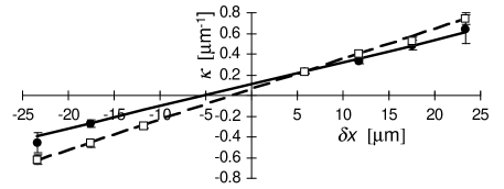
FIG. 3.: Plot of the spatial fringe frequency $\kappa$ versus $\delta x$ for $T_{0}$ = 1 ms (filled circles) and 4 ms (open squares). The solid and dashed lines are linear fits to the data.

Figure 3 plots the measured $\kappa$ vs. $\delta x$ [23] for $T_{0}$ = 1 and 4 ms. The data are well fit by a straight line as expected from Eq. (3) in the approximation that $\alpha$ and $\delta v$ are independent of $\delta x$. The slopes of the lines are the phase curvatures $\alpha$, and the $\kappa$ intercepts give the relative velocities $\delta v$.

We checked the validity of the data analysis procedure by analyzing data simulated with a 1-D Gross-Pitaevskii (GP) treatment. Despite variations of $\delta v$ and $\alpha$ with $\delta x$ (due to their continued evolution during the variable time $T_{2}$), we find that $\kappa$ is still linear in $\delta x$. The slopes and intercepts in general are averages over the range of $\delta x$ used in the experiment.

The interference fringes used to determine $\alpha$ and $\delta v$ are created at the time of the final interferometer pulse. Because the two outputs overlap at that moment, we wait a time $T_{3}$ for them to separate before imaging. During this time, the wavepackets continue to expand. The 1-D simulations show that the fringe spacings and the wavepackets expand in the same proportion. We correct $\kappa$ (by typically 15 $\%$) for this, using the calculated expansion from a 3-D solution of the GP equation described below.

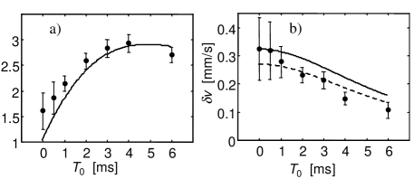
FIG. 4.: (a) Plot of the phase curvature $\alpha$ versus the initial expansion time $T_{0}$ showing the phase evolution from mean-field expansion. The solid line is a calculation using the Lagrangian Variational Method (LVM). (b) Plot of the relative repulsion velocity $\delta v$ versus $T_{0}$. The solid curve is the calculated maximum repulsion velocity (when $\delta x=0$) and the dashed curve is the repulsion velocity averaged over the range of $\delta x$ used in the experiment.

The different slopes and intercepts of the two lines in Fig. 3 show that the curvature $\alpha$ and relative velocity $\delta v$ of the wavepackets depend on the release time $T_{0}$ before the first interferometer pulse. Figure 4 plots the dependence of $\alpha$ and $\delta v$ on various release times $T_{0}$. The condensate initially has a uniform phase so that immediately after its release from the trap $\alpha=0$. We nevertheless measure a nonzero $\alpha$ for $T_{0}$ = 0 ms because the BEC expands during $T_{1}$ and $T_{2}$. As a function of time, $\alpha$ behaves as $\dot{D}$/$D$ where $D$ is the wavepacket diameter and $\dot{D}$ is its rate of change [20]. At early times when the mean-field energy is being converted to kinetic energy, $\dot{D}$ increases rapidly, increasing $\alpha$. At late times, after the mean-field energy has been converted, $D$ increases while $\dot{D}$ is nearly constant, decreasing $\alpha$.

We predict the time evolution of $\alpha$ using the Lagrangian Variational Method (LVM) [24]. The LVM uses trial wavefunctions with time dependent parameters to provide approximate solutions of the 3-D time-dependent GP equation. In the model, the effect of the interferometer pulses is to replace the original wavepacket with a superposition of wavepackets having different momenta; e.g., the action of our first interferometer pulse is $\psi_{0}\rightarrow\left(\psi_{0}+e^{i2kx}\psi_{0}\right)/\sqrt{2}$. We use Gaussian trial wavefunctions in the LVM and, for simplicity, neglect the interaction between the wavepackets, to calculate the phase curvature $\alpha$ at the time of the last interferometer pulse. This result, with $T_{1}=T_{2}$, is the solid line of Fig. 4a.

We use energy conservation to calculate the relative repulsion velocity $\delta v$ between $\psi_{A1}$ and $\psi_{B1}$ because we neglect wavepacket interactions in the LVM. In the Thomas-Fermi approximation, we can calculate the amount of energy available for repulsion when $T_{0}$ = 0. A trapped condensate has $\frac{5}{7}\mu$ average total energy per particle, where $\mu$ is the chemical potential [11]. After release from the trap, it has $\frac{2}{7}\mu$ average mean-field energy per particle. Applying a $\pi/2$ Bragg pulse to the BEC causes a density corrugation, which increases the mean-field energy to $\frac{3}{7}\mu$ per particle. In the approximation that the wavepackets do not deform as they separate and recombine, one can show that 1/3 of the total mean-field energy goes into expansion of the wavepackets, and 2/3 is available for kinetic energy of center-of-mass motion. Therefore $\frac{2}{7}\mu$ of mean-field energy per particle is available for repulsion. The corresponding repulsion velocity is only about $10^{-2}$ of a photon recoil velocity. The repulsion energy and $\delta v$ decrease for larger $T_{0}$ because both are inversely proportional to the condensate volume, which we calculate with the LVM. The two curves shown in Fig. 4b are the calculated $\delta v$ when $\delta x=0$ (solid curve) and $\delta v$ averaged over the different $\delta x$ used in the experiment (dashed curve). The 1-D GP simulations suggest that for small $T_{0}$, the results of the experiment should be closer to the solid curve; and for large $T_{0}$, closer to the dashed curve. The data is consistent with this trend.

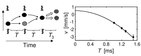
FIG. 5.: (a) Schematic representation of the interferometer in the trap, with the principle difference from Fig.  1 being the curved arrows indicating the acceleration of the wavepackets. (b) The relative velocity $v$ between the two trapped wavepackets versus the interferometer time $T$. The solid line is a fit.

In a related set of experiments we performed interferometry in the trap. This differs from the experiments on a released BEC because there is no expansion before the first interferometer pulse [25] and the magnetic trap changes the relative velocity of the wavepackets between the interferometer pulses (Fig. 5a). To better reveal the velocity differences, we choose $T_{1}$ = $T_{2}=T$ to suppress fringes arising from the phase curvature. As with the released BEC measurements, we observe equally spaced fringes at the output of the interferometer, although the fringes are almost entirely due to a relative velocity $v$ between the wavepackets $\psi_{{A1}}$ and $\psi_{{B1}}$ at the time of the third interferometer pulse. We obtain $v$ from the fringe periodicity after a small correction for residual phase curvature [26].

Two effects contribute to $v$: the mutual repulsion between the wavepackets $\psi_{{A}}$ and $\psi_{{B}}$ and the different action of the trapping potential on the two wavepackets in the interferometer. The latter effect occurs because after the first Bragg pulse, $\psi_{{A}}$ remains at the minimum of the magnetic potential while $\psi_{{B}}$ is displaced. Wavepacket $\psi_{{B}}$ therefore spends more time away from the center of the trap and experiences more acceleration than $\psi_{{A}}$.

Following the last Bragg pulse, $\psi_{{A1}}$ and $\psi_{{B1}}$ have a velocity difference which for our parameters can be approximated by $v\approx-\frac{2\hbar k}{M}{\rm sin^{2}}(\omega_{x}{T})+\delta v$ [27]. Figure 5b plots $v$ versus $T$, and the curve is a fit to the above expression. We obtain the trap frequency $\omega_{x}/2\pi=26.7(15)$ Hz, in excellent agreement with an independent measurement. We also obtain the relative velocity from the mean-field repulsion $\delta v=0.49(12)$ mm/s, which we expect to be somewhat larger than for the released measurements because the wavepackets contract, producing a larger mean field.

In conclusion, we demonstrate an autocorrelating matter-wave interferometer and use it to study the evolution of a BEC phase profile by analyzing spatial images of interference patterns. We study how the phase curvature of the condensate develops in time and measure the repulsion velocity between two BEC wavepackets. Our interferometric method should be useful for characterizing other interesting condensate phase profiles. For example, it can be applied to detect excitations of a BEC with characteristic phase patterns, such as vortices and solitons [14, 28, 29, 30, 31]. The method should be useful for further studies of the interaction of coherent wavepackets and to study the coherence of atom lasers.

We thank T. Busch, D. Feder, and L. Collins for helpful discussions. This work was supported in part by the US Office of Naval Research and NASA. J.D. acknowledges support from the Alexander von Humboldt foundation. M.E. and C.W.C. acknowledge partial support from NSF grant numbers 9802547 and 9803377.

REFERENCES

- [1] M. H. Anderson et al., Science 269, 198 (1995); K. B. Davis et al., Phys. Rev. Lett. 75, 3969 (1995); C. C. Bradley, C. A. Sackett, and R. G. Hulet, Phys. Rev. Lett. 78, 985 (1997); see also C. C. Bradley et al., Phys. Rev. Lett. 75, 1687 (1995).
- [2] M.-O. Mewes et al., Phys. Rev. Lett. 78, 582 (1997); E. W. Hagley et al., Science 283, 1706 (1999); I. Bloch, T. W. Hänsch, and T. Esslinger, Phys. Rev. Lett. 82, 3008 (1999); B. P. Anderson and M. A. Kasevich, Science 282, 1686 (1998).
- [3] P. R. Berman, Ed., Atom Interferometry (Academic Press, Cambridge, 1997).
- [4] M. R. Andrews et al., Science 275, 637 (1997).
- [5] J. Stenger et al., Phys. Rev. Lett. 82, 4569 (1999).
- [6] M. Kozuma et al., Phys. Rev. Lett. 82, 871 (1999).
- [7] E. W. Hagley et al., Phys. Rev. Lett. 83, 3112 (1999); M. Trippenbach et al., J. Phys. B 33, 47 (2000).
- [8] I. Bloch, T. W. Hänsch, and T. Esslinger, Nature 403, 166 (2000).
- [9] The mean-field energy shift of the out-coupled wavepacket in [5] can be used to infer the repulsion velocity. Here we measure the velocity directly.
- [10] All uncertainties reported here are 1 standard deviation combined statistical and systematic uncertainties.
- [11] F. Dalfovo et al., Rev. Mod. Phys. 71, 463 (1999).
- [12] D. M. Giltner, R. W. Mc Gowan, and S. A. Lee, Phys. Rev. Lett. 75, 2638 (1995).
- [13] Y. Torii et al., Phys. Rev. A 61, 041602(R) (2000).
- [14] J. Denschlag et al., Science 287, 97 (2000).
- [15] The condensate was imaged by first optically pumping the atoms to the ground state and then imaging the absorption of a probe beam on the transition. The pulse had a 5 s duration, 170 mW/cm2 intensity, and was detuned 15 MHz from resonance.
- [16] The momenta are not exactly and because of repulsion effects that will be discussed.
- [17] R. Trebino et al., Rev. Sci. Instrum. 68, 3277 (1997).
- [18] The observation is consistent with the full predicted fringe contrast when we include the finite imaging resolution.
- [19] We can treat the direction independently of and when the wavefunction is separable, i.e. . Straight fringes imply this separability.
- [20] Y. Castin and R. Dum, Phys. Rev. Lett. 77, 5315 (1996).
- [21] For ms and an interference pattern with many fringes, we found that the coefficients of third and fourth order terms are smaller than 1 m-3 and 1 m-4 respectively.
- [22] In practice, includes a random phase from mirror vibrations.
- [23] We use where = 5.9 cm/s is the two photon recoil velocity of sodium and is a small correction of the order due to the repulsion of the wavepackets. We include the correction in our data analysis in a self-consistent manner. The correction modifies insignificantly, but increases the final values of by 0.05 mm/s.
- [24] V. M. Pérez–Garcia et al., Phys. Rev. Lett. 77, 5320 (1996).
- [25] In fact, after the first pulse the wavepackets contract because the reduced mean-field energy can no longer support the wavepacket size.
- [26] We also correct the fringe spacings for the contraction of the wavepackets between the final interferometer pulse and when the image is taken.
- [27] We assume , , and harmonic motion in the trap.
- [28] S. Burger et al., Phys. Rev. Lett. 83, 5198 (1999).
- [29] M. R. Matthews et al., Phys. Rev. Lett. 83, 2498 (1999).
- [30] K. W. Madison et al., Phys. Rev. Lett. 84, 806 (2000).
- [31] A. D. Jackson, G.M. Kavoulakis, and C. J. Pethick, Phys. Rev. A 58, 2417 (1998).