Dynamic splitting of a Bose-Einstein condensate

Abstract

We study the dynamic process of splitting a condensate by raising a potential barrier in the center of a harmonic trap. We use a two-mode model to describe the phase coherence between the two halves of the condensate. Furthermore, we explicitly consider the spatial dependence of the mode funtions, which varies depending on the potential barrier. This allows to get the tunneling coupling between the two wells and the on-site energy as a function of the barrier height. Moreover we can get some insight on the collective modes which are excited by raising the barrier. We describe the internal and external degrees of freedom by variational ansatz. We distinguish the possible regimes as a function of the characteristic parameters of the problem and identify the adiabaticity conditions.

PACS numbers: 03.75.-b, 42.50.-p, 32.80.Pj

I Introduction

Bose-Einstein condensation of an ideal gas is typically presented in introductory textbooks solely in terms of particle numbers. And quantum mechanically enhanced number densities were the ‘smoking gun’ observed in the first experiments on dilute gas condensates. But many phenomena of interacting condensates depend critically on the conjugate quantity to particle number, namely the quantum mechanical phase [1, 2, 3, 4, 5]. One can have highly occupied states with or without phase coherence between them, and the presence or absence of phase coherence can make a dramatic difference in the physical properties of an ultra-cold gas. As in the case of a gas held in an optical lattice, which can be a superfluid or a Mott insulator depending on the strength of the lattice, the onset or loss of phase coherence can even be a phase transition [6].

Since the global phase of a condensate is unobservable, the simplest system in which phase coherence can be manifested consists of two states, occupied by a large number of bosons. As such a system can realistically be approximated by a condensate in a double well, it has recently attracted attention [7, 8, 9, 10, 11, 12, 13, 14, 15]. In these works, Josephson oscillations and the phase coherence between two coupled condensate were studied considering time independent coupling parameters. In [16] the disappearance of the phase coherence between the two wells due to a change in time of the tunneling coupling has been studied. The coupling parameters and the related phase coherence properties depend on the potential barrier between the two wells, since in the limit where the barrier is very low we have a single condensate and in the limit where the barrier is very high we have two completely separated condensates. Even if, at least in the high barrier limit, it has often been pointed out how to relate the coupling parameters (on-site energy and tunneling coupling) to the overlap of the wavefunctions localised in the two wells, this has never really been taken explicitly into account. Introducing the spatial degrees of freedom, as we did, allows us to relate all that to the potential barrier in a more than phenomenological way and becomes expecially important in the study of the dynamics of the process, because the wavefunctions change drastically in time and collective modes are excited.

In this paper we examine this problem and develop a method which can be extended to the case of many wells, in order to encompass the turning on of an optical lattice in a condensate, allowing to go beyond a Gross-Pitaevkii treatment, as the one done for example in [17]. The physical situation is similar to the ones already realized experimentally, where a double well potential was created by shining a far-off resonant laser beam in the center of the magnetic trap (see e.g. [18]) or where an array of traps was created by on optical standing wave [19].

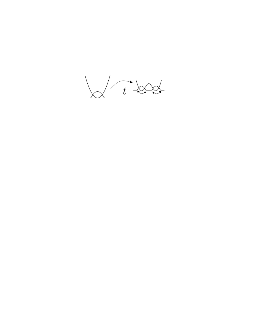
FIG. 1.: Schematic diagram of the process.

We are interested in the full dynamics of the process: in addition to the phase coherence properties, we want to study the excitation of the collective modes by taking the spatial dependence of the condensate wavefunction explicitly into account. The price of including all these effects without assuming mean field theory is that we must use a time-dependent variational approach, choosing variational ansatz to describe both the “internal” and “external” dynamics (that is, the distribution of particles between two motional states treated as given, and the evolution of the spatial wave functions of these states). This allows us to reduce the intractable full problem to a set of coupled differential equation for our few variational parameters. Although the time-dependent variational approach is not guaranteed to be quantitatively accurate, it allows qualitatively important processes to be investigated, and it has proven surprisingly reliable in previous applications to condensate physics [20]. Here we use it to derive the coupling between the internal and external dynamics, investigate which are the conditions under which the two can be decoupled, and identify the typical time scales for both.

In Sec. II we briefly present our two-state model and discuss qualitatively the behaviour of the system that our model can explain. In Sec. III, we introduce explicitly the variational ansatz we choose to describe the phase dynamics and the collective modes. After introducing the time–dependent variational principle and deriving the Lagrangian, we write the equations of motion for the variational parameters. Then in Sec. III E we discuss the conditions under which it is an accurate approximation to neglect the coupling between internal and external degrees of freedom. This decoupling allows us to model both internal and external evolution in a still simpler way. The external dynamics is studied in Sec. IV, comparing simple analytic models with numerical results. Sec. V is devoted to the internal dynamics, where the statics is studied and analytic estimates obtained. With these decoupled studies to guide expectations, the full variational equations of motion, with coupled internal and external degrees of freedom, will be studied numerically in Sec. VI. The results are compared with those of the phase model describing the relative phase of two weakly coupled superfluids [21, 22]. We conclude with a general discussion of our results and their implications. Two appendices define the number difference and relative phase operators , derive the phase model Hamiltonian, and show that our variational ansatz adequately represents the evolution generated by it.

II Model

Let us consider the situation in which we have $N$ bosons confined in a harmonic trap at zero temperature. We slowly deform the trap symmetrically around its center raising a potential barrier, until it becomes a double–well potential. We want to study the dynamics of the process as well as the final state of the bosons.

We will treat the problem in one dimension. This describes the situation in which we have a cigar-shaped condensate, and we deform it along the most elongated direction. Nevertheless, our model could be extendend in a straightforward way to $2$ and $3$ dimensions. This would just lead to more complicated equations, but would not affect the main results.

A Two–mode model

The second quantization Hamiltonian describing the situation we have in mind and in which particles interact via a $\delta$-pseudopotential is

$$\hat{H}(t) = \int\hat{\Psi}^{{\dagger}}(z)\left(\frac{p^{2}}{2M}+V(z,t)\right)\hat{\Psi}(z)dz+$$ (1)

$$+ \frac{1}{2}\;g\int\hat{\Psi}^{{\dagger}}(z)\hat{\Psi}^{{\dagger}}(z)\hat{\Psi}(z)\hat{\Psi}(z)dz,$$ (2)

where $\hat{\Psi}$ is the bosonic field operator and $V(z,t)$ is the time–dependent potential which describes the deformed trap. Here, $g$ is an effective coupling constant which depends both on the $s$-wave scattering length and on the atomic distribution in the transverse directions.

We assume that at time $t=0$ the atoms are in the ground state of this Hamiltonian, and we want to determine the state after the potential is deformed. This problem cannot be solved even numerically (see, for example, [23] and references therein). Therefore, we need to consider a simplified model which describes the main features of the process. If the process is completely adiabatic, the final state will be a ‘fragmented condensate’ with half of the particles in each of the potential wells: when the two condensates do not interact this is a much lower energy state than the one with phase coherence, because minimizing fluctuations in the relative particle number lowers the energy due to interparticle repulsion. Such a fragmented condensate can be regarded as having two entirely independent condensates. If we changed the potential very fast, then we would obtain a single condensate that oscillates in each of the potential wells. We would also expect to see collapses and revivals in the “condensate phase” [1], provided the losses are not important [24].

It is clear that the Gross–Pitaevskii Equation (GPE) will not give a good description of the splitting process, in principle. This equation describes the evolution of a single mode of the condensate $\varphi(z,t)$, and, therefore, is not valid for fragmented condensates. In order to interpolate between the Gross-Pitaevskii limit of phase coherence and the limit of two independent condensates, one needs to consider at least two modes $\varphi_{1,2}(z,t)$. Then, one can write the state of the atoms as (we assume $N$ to be even)

$$|\Phi(t)\rangle = \sum_{m=-N/2}^{N/2}c_{m}(t)|m(t)\rangle,$$ (3)

where

$$|m(t)\rangle = \frac{a_{1}(t)^{{\dagger}\frac{N}{2}-m}}{\sqrt{\left(\frac{N}{2}-m\right)!}}\frac{a_{2}(t)^{{\dagger}\frac{N}{2}+m}}{\sqrt{\left(\frac{N}{2}+m\right)!}}|vac\rangle,$$ (4)

and $a_{1,2}$ are the mode annihilation operators defined as

$$a_{i}^{{\dagger}}(t)=\int\varphi_{i}(z,t)\Psi^{{\dagger}}(z)\,dz.$$ (5)

We have to consider the evolution of the wavefunctions $\varphi_{1,2}$ as well as of the coefficients $c_{m}$, which will be coupled and governed by the Hamiltonian

$$\hat{H}(t)=$$ (6)

$$=\sum_{ij=1,2}a_{i}^{{\dagger}}a_{j}\int\varphi_{i}^{*}(z,t)\left(\frac{p^{2}}{2M}+V(z,t)\right)\varphi_{j}(z,t)dz$$ (7)

$$+\frac{g}{2}\sum_{ijlm=1,2}a_{i}^{{\dagger}}a_{j}^{{\dagger}}a_{l}a_{m}$$ (8)

$$\hskip 56.9055pt\int\varphi_{i}^{*}(z,t)\varphi_{j}^{*}(z,t)\varphi_{l}(z,t)\varphi_{m}(z,t)dz.$$ (9)

We will refer to the evolution of those wavefunctions as “external dynamics” and to the one of the coefficients as “internal dynamics”.

In order to find the mode–functions $\varphi_{1,2}$ we can use the variational principle (in the same way as one derives the GPE from a Hartree-Fock ansatz). However, this also turns out to be very complicated. A way around that problem is to express $\varphi_{1,2}$ in terms of some few variational parameters: we will use quasi–gaussian functions to describe those mode-functions. On the other hand, we could also use a variational principle to determine the evolution of the coefficients $c_{m}$. This again turns out to be very complicated, so that we will also use a Gaussian ansatz for them. Once they are known, in order to estimate when the condensate is fragmented, we can look at the eigenvalues of the single particle density operator corresponding to the internal dynamics only, that is, the matrix

$$\rho=\frac{1}{N}\left(\begin{array}[]{c c}\langle a_{1}^{{\dagger}}a_{1}\rangle&\langle a_{1}^{{\dagger}}a_{2}\rangle\\ \langle a_{2}^{{\dagger}}a_{1}\rangle&\langle a_{2}^{{\dagger}}a_{2}\rangle\end{array}\right),$$ (12)

where $\langle a_{i}^{{\dagger}}a_{j}\rangle$ mean the expectation value on the state $|\Phi\rangle$. The eigenvalues $\lambda_{\pm}$ indicate whether we have a single condensate ($\lambda_{+}\sim 1$, $\lambda_{-}\sim 0$), or a fragmented one ($\lambda_{+}\sim\lambda_{-}\sim 1/2$).

As already extensively discussed in the literature [7, 16], the two-mode model has a limited validity in the case of low barrier, when in principle one is not allowed to neglect higher excited modes. However, it becomes more and more accurate the higher the barrier gets, since in this case the two lower lying modes move closer together in energy compared to the higher ones. Hence it should allow a good description of the splitting process.

B Qualitative behavior

Before presenting the numerical and analytical result coming from our analysis, we will briefly discuss the qualitative behavior that we expect from the model under study. We will show that the equations we will derive for the external and internal dynamics can be decoupled to a very good approximation. That is, we can first solve the equations for the external dynamics basically taking constant values for the variational parameters describing the coefficients $c_{m}$. Once these equations are solved, we can use the corresponding wavefunctions $\varphi_{1,2}$ to calculate the time–dependent coefficients for the equations that describe the internal variational parameters. In summary, once we have solved the equations for the external parameters, we are left with a two–mode model with time–dependent coefficients which contain all information about the external dynamics: they will define the hopping and on-site interaction, whose competition determines the phase relation between the two modes.

Regarding the external dynamics, one can see two kinds of behaviors depending on the time scale $\tau$ at which the barrier is raised. The important time scale with which one has to compare is the oscillation period $\tau_{z}$ in the trapping potentials at each time. These periods change by roughly a factor of two between the initial harmonic potential and the final double well (with our specific choice of the trapping potential). Thus, if $\tau\gg\tau_{z}$ the process will be adiabatic with respect to the external dynamics, which means that $\varphi_{1,2}(z,t)$ will basically correspond to the two ground states of the right and left wells at the final time. If $\tau\ll\tau_{z}$ we will have collective excitations, in which $\varphi_{1,2}(z,t)$ oscillate strongly. In this case, we will have that the energy of the condensate $E$ (with respect to the ground state energy) has increased, so that it may be destroyed. Although we cannot account for the disappearance of the condensate within our model, we can estimate when this will happen just by considering the fact that under normal circumstances thermalization will occur, and, therefore, the condensate will be destroyed for $E=K_{B}T_{c}>N\hbar\omega_{z}$, where $\omega_{z}=2\pi/\tau_{z}$, $K_{B}$ is the Boltzman constant, $T_{c}$ indicates the critical temperature and $E$ is the extra energy in the final state. We find that the condensate disappears for $\tau\simeq\tau_{z}$.

Regarding the internal dynamics, there is also a time scale in the problem which determines the dynamics; this is the revival time $\tau_{r}$. Given two condensates with an initial well defined relative phase, it is well–known that the relative phase first disappears (collapse) and then is restored at time $\tau_{r}\sim 1/g$ [3, 4]. If $\tau\gg\tau_{r}$ the process will be adiabatic with respect to the internal dynamics, the phase coherence will be lost during the process and therefore we will end up with two independent condensates in each well, with no phase coherence at all (note that it makes no sense to talk about collapses or revivals in this situation). If $\tau\ll\tau_{r}$ at the end of the process we will have two condensates with a good phase coherence. In that case, after the splitting, collapses and revivals could be observed provided the particle losses are practically absent.

In summary, we have two important time scales in the problem, namely $\tau_{z}$ and $\tau_{r}$. Typically, in experiments $\tau_{r}\gg\tau_{z}$, so that it will be harder to be adiabatic with respect to the internal dynamics than to the external one. On the other hand, since $\tau_{r}$ is very long in practise, it will be hard to achieve $\tau\gg\tau_{r}$ within the validity of our model, in which particle losses and other imperfections are not included.

Finally we notice that the external and internal dynamics depend in a very different way on the parameters $g$ and $N$. Very similar to what happens in the GPE, the equations of motion for the parameters describing the external dynamics depend almost only on the product $gN$. On the contrary, the on-site energy splitting scales like $g$ and the tunneling coupling like $N$ giving rise to very different internal dynamics. For increasing $N$ and decreasing $g$ the relative phase becomes better defined and the time $\tau_{r}$ required to destroy the phase coherence is longer. In particular in the limit $N\rightarrow\infty$, unless the tunneling coupling exactly vanishes, the GPE case of phase coherent condensate is recovered.

III Variational ansatz

In this Section we introduce a variational ansatz to describe the internal and external dynamics. To describe the ground state of the system, which we will call equivalently static or equilibrium solution, two parameters are sufficient: $z_{0}$ which corresponds roughly to the center of the mode functions, and $p$ which is related to the width of the number distribution. To allow dynamic evolution we have to introduce also the variables $\sigma_{I}$ and $x_{I}$, which will vanish in the static case. For simplicity in the following we present the variational ansatz for the symmetric case, describing a spatially symmetric double–well potential and a symmetric atomic distribution among the two modes. Starting from symmetric initial conditions (no unbalance in the population of the two modes and symmetric mode functions $\varphi_{1}(z)=\varphi_{2}(-z)$), the symmetry will be preserved under the time evolution. Nevertheless, it is possible to generalize our ansatz to describe asymmetric situations. We will briefly discuss the corresponding results in the conclusions.

A Variational ansatz for the mode functions

For a single condensate in a harmonic trap, a Gaussian ansatz for the wavefunction has proved to be very useful and able to predict the excitation frequencies within a very high precision [20]. In our case we make a similar choice. For a very high barrier we expect to find two separate condensates for each of which a Gaussian ansatz should be good. We then define the two functions for the left and right side:

$$\varphi_{R,L}(z)=$$ (13)

$$= \left(\frac{\sigma_{R}}{\pi}\right)^{1/4}\exp\left[-\frac{\sigma_{R}(z\mp z_{0})^{2}}{2}\right]\exp\left(-i\frac{\sigma_{I}}{2}z^{2}\right).$$ (14)

In the case of low barrier (small $z_{0}$), these two functions have to be orthogonalized to satisfy the orthonormality property required for the two mode functions. Hence we define

$$\varphi_{\pm}(z) = \frac{1}{\sqrt{2}\sqrt{1\pm\exp(-\sigma_{R}z_{0}^{2})}}\left(\varphi_{R}\pm\varphi_{L}\right),$$ (16)

$$\varphi_{1,2}(z) = \frac{1}{\sqrt{2}}\left(\varphi_{+}\pm\varphi_{-}\right),$$ (17)

which are different from $\varphi_{R,L}$ because of the two different normalization constants for $\varphi_{+}$ and $\varphi_{-}$.

The variational parameters describing the mode functions $\varphi_{1,2}$ are $z_{0}$ and $\sigma_{I}$. Physically, the excitation modes that these parameters can describe depend on whether the two Gaussians significantly overlap in space or not. If they do, as in the case of low barrier, then the excitation mode (changes in $z_{0}$) corresponds to a breathing mode. If they do not overlap, as for high barrier, then it corresponds to an oscillation mode in each of the potential wells. Allowing also $\sigma_{R}$ to vary (and adding an extra variable for the dynamics) one can describe more excitation modes. Instead we fix it to a constant value, since the curvature of the potential wells will be chosen to be always of the same order of magnitude. The value of $\sigma_{R}$ is not obvious since the overlap integrals depend strongly on it. For instance the hopping terms can be overestimated due to the long Gaussian tales. To fix $\sigma_{R}$, we identified a range of values for which the dynamic behaviour of the system was qualitatively the same and choose one of the values within this interval, which turned out to be lower than the one corresponding to the static solution.

Since the mode wavefunctions are linear combinations of Gaussians, if we choose a trapping potential of the form

$$V(z)=\frac{1}{2}M\omega_{T}^{2}z^{2}+V_{0}(t)\exp[-z^{2}/a(t)],$$ (18)

the integrals in Eq.(V A) can be performed analytically.

In the following, we will use dimensionless units: $a_{ho}=\sqrt{\hbar/M\omega_{T}}=1$, $\hbar\omega_{T}=1$ and $\hbar=1$. So, all lengths will be measured in units of harmonic oscillator length, all energy in units of the trap frequency and all times in units of $\omega_{T}^{-1}$.

B Variational ansatz for the coefficients

We also take for the coefficients $c_{m}(t)$ a Gaussian distribution centered at $m=0$,

$$c_{m} = {\cal N}(p)\exp\left[-\left(\frac{1}{4{p}}+i{x_{I}}\right)m^{2}\right],$$ (19)

where ${\cal N}(p)$ is a normalization constant that depends on $p$ only. The variational parameters are $p$ and its conjugate one $x_{I}$. The parameter $p$ is directly related to the width of the distribution $|c_{m}|^{2}$, whereas $x_{I}$ contributes to the width of the Fourier transform of such a distribution (i.e., to the width of the phase distribution, see App. A).

C Time-dependent variational principle

We study the dynamics using the time dependent variational principle. To derive the equations of motion one starts by writing the action $S$

$$S=\int dt\frac{\langle\dot{\Phi}|\Phi\rangle-\langle\Phi|\dot{\Phi}\rangle}{2i}-\langle\Phi|\hat{H}|\Phi\rangle.$$ (20)

where ${\hat{H}}$ and $|\Phi\rangle$ have been defined in (6) and (3), respectively. In evaluating the term $\langle\Phi|\dot{\Phi}\rangle$, one should remember that the state $|\Phi\rangle$ depends on time both through the coefficients and the mode functions contained in $|m\rangle$:

$$\langle{\dot{\Phi}}|\Phi\rangle=\sum_{m}{\dot{c}}_{m}^{*}c_{m}+\sum_{mm^{\prime}}c_{m^{\prime}}^{*}c_{m}\langle{\dot{m}}^{\prime}|m\rangle.$$ (21)

The Lagrangian which follows takes the form

$$L = \frac{1}{2i}\left[\sum_{m}{\dot{c}}_{m}^{*}c_{m}+\right.$$ (23)

$$\left.\hskip 28.45274pt+\sum_{ij}\langle a_{i}^{{\dagger}}a_{j}\rangle\int{\dot{\varphi}}_{i}^{*}\varphi_{j}dz-h.c.\right]-{\cal H},$$

where ${\cal H}\equiv\langle\Phi|{\hat{H}}|\Phi\rangle$ is given by

$${\cal H}=$$ (24)

$$=\sum_{ij=1,2}\langle a_{i}^{{\dagger}}a_{j}\rangle\int\varphi_{i}^{*}(z,t)\left(\frac{p^{2}}{2M}+V(z,t)\right)\varphi_{j}(z,t)dz$$ (25)

$$+\frac{1}{2}\;g\sum_{ijlm=1,2}\langle a_{i}^{{\dagger}}a_{j}^{{\dagger}}a_{l}a_{m}\rangle$$ (26)

$$\hskip 56.9055pt\int\varphi_{i}^{*}(z,t)\varphi_{j}^{*}(z,t)\varphi_{l}(z,t)\varphi_{m}(z,t)dz.$$ (27)

From the Lagrangian (23), in general one derives the equations of motion, carrying out the variation with respect to the discrete variables $c_{m}$ and the fields $\varphi_{i}$. In our case, all the integrals and expectation values are functions of the variational parameters which can be calculate analytically. The only important overlap integrals containing time derivatives are

$$\int\dot{\varphi}_{1,2}^{*}\varphi_{1,2}dz = -\frac{i}{2}\left(\frac{1}{\sigma_{R}}+\frac{z_{0}^{2}}{1-e^{-2\sigma_{R}z_{0}^{2}}}\right)\dot{\sigma}_{I},$$ (29)

$$\int\dot{\varphi}_{1,2}^{*}\varphi_{2,1}dz = \frac{i}{2}\frac{z_{0}^{2}e^{-2\sigma_{R}z_{0}^{2}}}{1-e^{-2\sigma_{R}z_{0}^{2}}}\dot{\sigma}_{I}.$$ (30)

If one defines

$$N_{\phi}=\langle a_{1}^{{\dagger}}a_{2}\rangle+\langle a_{2}^{{\dagger}}a_{1}\rangle$$ (31)

and

$${\cal I}(p,x_{I},z_{0})\equiv$$ (32)

$$= \frac{N}{2}\left(\frac{1}{\sigma_{R}}+\frac{z_{0}^{2}}{1-e^{-2\sigma_{R}z_{0}^{2}}}\right)-\frac{N_{\phi}}{2}\frac{z_{0}^{2}e^{-2\sigma_{R}z_{0}^{2}}}{1-e^{-2\sigma_{R}z_{0}^{2}}},$$ (33)

the Lagrangian becomes

$$L = p\dot{x}_{I}+{\cal I}\dot{\sigma}_{I}-\cal{H},$$ (34)

and the corresponding equations of motion are

$$\left(\begin{array}[]{c c c c}0&-1&0&-\frac{\partial{\cal I}}{\partial p}\\ 1&0&0&-\frac{\partial{\cal I}}{\partial x_{I}}\\ 0&0&0&-\frac{\partial{\cal I}}{\partial z_{0}}\\ \frac{\partial{\cal I}}{\partial p}&\frac{\partial{\cal I}}{\partial x_{I}}&\frac{\partial{\cal I}}{\partial z_{0}}&0\end{array}\right)\left(\begin{array}[]{c}\dot{p}\\ \dot{x}_{I}\\ \dot{z}_{0}\\ \dot{\sigma}_{I}\end{array}\right)=-\left(\begin{array}[]{c}\frac{\partial{\cal H}}{\partial p}\\ \frac{\partial{\cal H}}{\partial x_{I}}\\ \frac{\partial{\cal H}}{\partial z_{0}}\\ \frac{\partial{\cal H}}{\partial\sigma_{I}}\end{array}\right)$$ (47)

$$\Rightarrow \left\{\begin{array}[]{r c l}\dot{p}&=&-\frac{\partial{\cal H}}{\partial x_{I}}+\frac{\partial{\cal I}}{\partial x_{I}}\dot{\sigma}_{I}\\ -\dot{x}_{I}&=&-\frac{\partial{\cal H}}{\partial p}+\frac{\partial{\cal I}}{\partial p}\dot{\sigma}_{I}\\ \frac{\partial{\cal I}}{\partial z_{0}}\dot{z}_{0}&=&-\frac{\partial{\cal H}}{\partial\sigma_{I}}-\left(\frac{\partial{\cal I}}{\partial p}\dot{p}+\frac{\partial{\cal I}}{\partial x_{I}}\dot{x_{I}}\right)\\ -\frac{\partial{\cal I}}{\partial z_{0}}\dot{\sigma}_{I}&=&-\frac{\partial{\cal H}}{\partial z_{0}}\end{array}\right.$$ (52)

These equations describe the internal and external coupled dynamics of the splitting of the condensate. In what follows, we have solved them numerically in different regimes. Before presenting the results we will show that one can decouple the evolution of the external and internal variables, which helps to understand the dynamics. For that, we will introduce in the next subsection some analytical approximations to derive explicit formulae for the quantities ${\cal H}$ and ${\cal I}$ by replacing the discrete distribution $c_{m}$ by a continuous one, and treating the index $m$ as a continuous variable running from $-\infty$ to $\infty$.

D Continuous limit

In order to calculate ${\cal H}$ and ${\cal I}$ we have to evaluate expectation values of the form $\langle a_{i}^{\dagger}a_{j}\rangle$ and $\langle a_{i}^{\dagger}a_{j}^{\dagger}a_{l}a_{m}\rangle$. We can do that if we replace the sums in $m$ by integrals extended from $-\infty$ to $\infty$. When this replacement is valid, we can even calculate the width of the number distribution $|c_{m}|^{2}$, $\sigma_{m}$, as well as the one corresponding to the phase distribution, $\sigma_{\phi}$ (see App.A). We obtain

$$\sigma_{m} = \sqrt{p},$$ (54)

$$\sigma_{\phi} = \sqrt{\frac{1}{4p}+4px_{I}^{2}}.$$ (55)

On the other hand, we have

$$\langle a_{1,2}^{{\dagger}}a_{1,2}\rangle=\frac{N}{2},$$ (57)

$$\langle a_{1,2}^{{\dagger}2}a_{1,2}^{2}\rangle=\frac{N^{2}}{4}+p,$$ (58)

$$\langle a_{1}^{{\dagger}}a_{2}\rangle=\langle a_{2}^{{\dagger}}a_{1}\rangle^{*}=$$ (59)

$$\hskip 14.22636pt=\frac{N}{2}\exp\left(-\frac{\sigma_{\phi}^{2}}{2}\right)\left[1-\frac{2p}{N^{2}}+\frac{8p^{2}x_{I}^{2}}{N^{2}}\right],$$ (60)

$$\langle a_{1}^{{\dagger}}a_{2}^{{\dagger}}a_{1}a_{2}\rangle=\frac{N^{2}}{4}-p,$$ (61)

$$\langle a_{1}^{{\dagger}2}a_{2}^{2}\rangle=$$ (62)

$$\hskip 14.22636pt=\frac{N^{2}}{4}\exp\left(-2\sigma_{\phi}^{2}\right)\left[1-\frac{4p}{N^{2}}+\frac{64p^{2}x_{I}^{2}}{N^{2}}\right].$$ (63)

Furthermore, in this limit we can determine the eigenvalues of the single particle density operator corresponding to the internal degrees of freedom, obtaining

$$\lambda_{\pm}\approx\frac{1\pm\exp\left(-\sigma_{\phi}^{2}/2\right)}{2}.$$ (64)

Notice that $\lambda_{+}\rightarrow 1$ for $p\sim N/4,x_{I}\sim 0$, i.e. $\sigma_{\phi}\sim 0$, which corresponds to the Gross-Pitaevskii limit; instead $\lambda_{\pm}\rightarrow 1/2$ for large $\sigma_{\phi}$, giving a signature of the fragmentation of the condensate.

One can easily determine the limits of validity of this continuous approximation. On the one hand, the distribution in $c_{m}$ has to be sufficiently broad, which implies $p\gtrsim 1$. On the other hand, $x_{I}$ has to be such that $\sigma_{\phi}\lesssim\pi$. For our numerical simulations, we corrected the expressions in Eqs.(III D) to make them valid $\forall p$ and $\forall x_{I}$: for $p>1$ we included the periodicity in $x_{I}$ and for $p<1$ we performed the exact sum over $m$, considering only the few number states which are populated.

E Decoupling between external and internal dynamics

The coupling among the $z_{0}$ dynamics and the $p$ dynamics appears in the off-diagonal blocks in Eq.(47) and in the dependence of ${\cal H}$ on all variational parameters. In the following we will analyze under which condition it is possible to decouple the internal ($p,x_{I}$) and external ($z_{0},\sigma_{I}$) dynamics, so that one can study them independently one from the other.

1 External dynamics

One can rewrite the equation of motion for $z_{0}$ is a more explicit form as

$$\frac{\partial{\cal I}}{\partial z_{0}}\dot{z}_{0} = -\frac{\partial\cal{H}}{\partial\sigma_{I}}+\frac{1}{2}\frac{z_{0}^{2}\exp(-\sigma_{R}z_{0}^{2})}{1-\exp(-2\sigma_{R}z_{0}^{2})}\dot{N}_{\phi}.$$ (65)

Let us first see under which circumstances it is possible to neglect the off-diagonal blocks:

(i) in the low barrier limit, i.e. $\exp(-\sigma_{R}z_{0}^{2})\sim 1$, the off-diagonal blocks can be neglected if ${\dot{N}}_{\phi}$ plays no role: $N_{\phi}$ evolves at the frequency which governs the internal dynamics $\omega_{p}$ (remember definition (31)), while the external dynamics is governed by the frequency $\omega_{z}$, usually of the order of the trapping frequency $\omega_{T}$. If $\omega_{p}\gg\omega_{z}$, then the time average of $\dot{N}_{\phi}$ vanishes and has no effect on the evolution of $z_{0}$. On the other hand $\omega_{p}\sim gNU_{1}\exp(-\sigma_{R}z_{0}^{2}/2)\lesssim\omega_{z}$ only for a chemical potential $\mu\sim gNU_{1}\lesssim\omega_{T}$. This happens either for very few particles, a case in which our model does not hold, since $N\gg 1$ is a fundamental assumption in our model, or for very weakly interacting particles, in which ${\dot{N}}_{\phi}\sim 0$, because the phase coherence is very difficult to be destroyed.

(ii) in the high barrier limit, normally $\omega_{p}\ll\omega_{z}$ (see Fig. 5, small $p$ limit) and $N_{\phi}$ might vary abruptly, since this is when the phase coherence is supposed to desappear. Anyway, since $\exp(-\sigma_{R}z_{0}^{2})\sim 0$, the off-diagonal block can be neglected.

Now let us analyze the $p$–$x_{I}$ dependence in ${\cal H}$ (see Eqs.(24,III D)). In the on-site terms this dependence is of order $p/N^{2},x_{I}/N^{2}\ll 1$ and can be therefore safely neglected (Eqs.(57,58)). In the hopping terms, it scales like $\exp(-\sigma_{\phi}^{2}/\alpha)$ ($\alpha=2,1/2$, see Eqs.(59,62)): it is strong only when the hopping terms are already small and negligible in comparison with the on-site terms, so it can also be neglected.

After these considerations, we conclude that the $z_{0}$-dynamics is, in a good approximation and in reasonable regimes, independent of the $p$-dynamics. This is confirmed by the numerical simulations.

2 Internal dynamics

The off-diagonal blocks can be neglected in the $p$-dynamics if $\partial{\cal H}/\partial z_{0}\sim 0$ or $\exp(-\sigma_{R}z_{0}^{2})\sim 0$. If the barrier is raised starting from a condensate in the ground state, $z_{0}$ evolves almost adiabatically in the low barrier limit ($\partial{\cal H}/\partial z_{0}\sim 0$); when it reaches the high barrier limit, then $\exp(-\sigma_{R}z_{0}^{2})\sim 0$. Therefore, the off-diagonal terms can be neglected during the whole process.

Instead, the $z_{0}-\sigma_{I}$ dependence in ${\cal H}$ is strong. One can solve the complete coupled dynamics or substitute in ${\cal H}$ the adiabatic solution for $z_{0}$ and compare the results. We will show some examples in the following and see that the difference is small.

IV External dynamics: excitations

In the previous section, we have written the equations of motion describing the full coupled dynamics and demonstrated that if one splits a condensate starting from a ground state configuration, it is possible to decouple the internal and the external dynamics. In this section, we will use this result and study the external dynamics decoupling it from the internal one. Making use of the external static solution, in Sec. V we will discuss the static solution for the internal degrees of freedom. Finally in Sec. VI, we show the results for the internal dynamics, which are also useful as a check of the decoupling assumption.

The fact that the internal and external dynamics decouple under the condition discussed above, allows us to estimate the excitation of the collective modes using a very simple model. We point out that in this case, similarly to the Gross-Pitaesvkii equation, the external dynamics is governed by the product $gN$ and not by the two quantities separately.

We choose to raise the potential barrier with the following time dependence

$$V_{0}(t)=\frac{V_{0fin}}{2}\left(\tanh\frac{t}{\tau}+1\right).$$ (66)

From the static solution, obtained by minimizing ${\cal H}(p,x_{I},z_{0},\sigma_{I},V_{0})$ with respect to all variational parameters simultaneously at fixed $V_{0}$, we know the equilibrium position of $z_{0}$ at any value of the barrier. The $z_{0}$ dynamics can be approximated very well by the dynamics in a harmonic potential whose center moves from $z_{0in}$ to $z_{0fin}$ following the adiabatic solution and whose frequency changes corresponding to the frequency of the small oscillations.

To get analytic estimations, we model this dynamics by fixing the frequency and shifting the center of the potential along a trajectory $z_{c}(t)$ for which an analytic solution exists. When the center follows an hyperbolic tangent trajectory with time constant $\tau$, the semi-amplitude of the oscillation is given by

$$\delta z_{0}=$$ (67)

$$\left(z_{0fin}-z_{0in}\right)\frac{\pi\omega\tau}{4}{\rm csch}\left(\frac{\pi\omega\tau}{4}\right){\rm sech}\left(\frac{\pi\omega\tau}{4}\right).$$ (68)

Otherwise, if the center moves according to a linear ramp with time constant $\tau$, the average semi-amplitude of the oscillation is

$$\delta z_{0} = \sqrt{2}\frac{z_{0fin}-z_{0in}}{\omega\tau}.$$ (69)

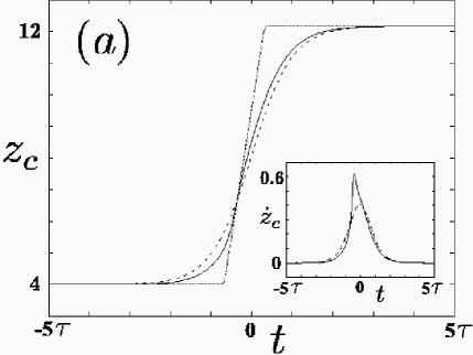
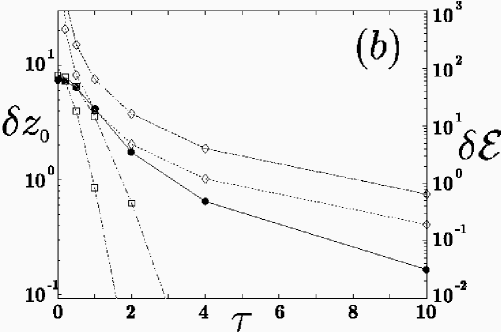
FIG. 2.: (a) Static solution for $z_{0}$ (full line) and position for the center of the harmonic potential for a raising time scale $\tau$: hyperbolic tangent shift (dashed line) and linear shift (dotted line); time derivative of $z_{0}(t)$ (inset). (b) Semi-amplitude of the final oscillations (left axis) and final excitation energy per particle (right axis): numerical results ($\bullet$), results for the $\tanh$ ($\Box$) and linear shift ($\diamond$) for $\omega=2.82$ and $1.54$.

We compare in Fig.2 these expressions with the numerical results. For fast raising of the barrier the hyperbolic tangent shift gives a good estimate. For slower raising, instead, the amplitude of the oscillations is largely underestimated. In this case, the linear shift of the center is useful to give an upper bound. We have checked numerically (by changing the frequency of the harmonic potential in time according to the adiabatic solution) that the small discrepancy between the actual shift of the center and the hyperbolic tangent dependence is enough to produce such a big change in the amplitude of the final oscillations. The reason for this might be better understood comparing the time derivative of $z_{c}(t)$ in the two cases (see inset in Fig.2(a)). Our estimations are qualitative, but allow us to set some lower and upper bounds and deduce an adiabaticity condition $\tau\ll 1/\omega_{z}$ for the external degrees of freedom. In the same way we can estimate the extra energy per particle due to the excitation of collective modes. Using the relation $K_{B}T_{c}\sim N\hbar\omega_{z}$ (the trapping frequency at the end of the process is $\omega_{z}$ and not $\omega_{T}$), we can estimate which is the fastest time scale which does not destroy the condensate. As expected, it is $\tau\sim 1/\omega_{z}$.

V Internal dynamics: static solution

In this section, we will study the complete splitting process, starting from a condensate trapped in a harmonic potential and ending with a potential barrier with height $V_{0}$. Apart from presenting the numerical results obtained by solving Eqs.(47), we will also introduce a simple two–mode model that allows a deeper understanding of the results obtained by the variational ansatz.

A Two–mode model

Given the fact that the external dynamics is basically independent of the internal one, we can derive a simple model that accounts for most of the effects related to the internal dynamics. The Hamiltonian in Eq.(6) depends on the following overlap integrals

$$K_{ij} = \int\varphi_{i}^{*}(z)\frac{p^{2}}{2M}\varphi_{j}(z)dz,\hskip 14.22636pt$$ (71)

$$V_{ij} = \int\varphi_{i}^{*}(z)V(z)\varphi_{j}(z)dz,$$ (72)

$$U_{1} = \int|\varphi_{i}(z)|^{4}dz,$$ (73)

$$U_{2} = \int|\varphi_{i}(z)|^{2}|\varphi_{j}(z)|^{2}dz=$$ (74)

$$= \int\varphi_{i}^{*}(z)\varphi_{i}^{*}(z)\varphi_{j}(z)\varphi_{j}(z)dz,$$ (75)

$$U_{3} = \int|\varphi_{i}(z)|^{2}\varphi_{i}^{*}(z)\varphi_{j}(z)dz,$$ (76)

where $i,j=1,2$ [27]. We use

$$a_{1}^{{\dagger}}a_{1}^{{\dagger}}a_{1}a_{2}+a_{1}^{{\dagger}}a_{2}^{{\dagger}}a_{2}a_{2}=$$ (77)

$$=\left(a_{1}^{{\dagger}}a_{1}-1+a_{2}^{{\dagger}}a_{2}\right)a_{1}^{{\dagger}}a_{2}\approx Na_{1}^{{\dagger}}a_{2},$$ (78)

to define two effective single-particle hopping terms $J_{12}=-K_{12}-V_{12}-gNU_{3}=-K_{21}-V_{21}-gNU_{3}$. The static solution for the external dynamics is known from the minimization of ${\cal H}(p,x_{I},z_{0},\sigma_{I},V_{0})$. Plugging the corresponding solution $z_{0}(V_{0})$ in Eqs.(V A), we get Hamiltonian parameters depending only on the barrier height $V_{0}$ (in particular $J_{12}=J_{21}=J$). Neglecting constant terms, we write the simplified Hamiltonian

$${\hat{H}} = \frac{1}{2}gU_{1}\left[a_{1}^{{\dagger}2}a_{1}^{2}+a_{2}^{{\dagger}2}a_{2}^{2}\right]-J\left[a_{1}^{{\dagger}}a_{2}+a_{2}^{{\dagger}}a_{1}\right]+$$ (79)

$$+ 2gU_{2}a_{1}^{\dagger}a_{2}^{\dagger}a_{1}a_{2}+\frac{1}{2}gU_{2}\left[a_{1}^{{\dagger}2}a_{2}^{2}+a_{2}^{{\dagger}2}a_{1}^{2}\right].$$ (80)

As it is well–known (see App. A), under certain conditions we can replace this model Hamiltonian by a phase model of the form

$${\hat{H}} = -g\left(U_{1}-2U_{2}\right)\frac{\partial^{2}}{\partial\phi^{2}}-JN\cos\phi+$$ (82)

$$+g\frac{N^{2}}{4}U_{2}\cos 2\phi\,,$$

where $\phi$ represents the relative phase between the two modes. The overlap integral $U_{2}$ may be non-negligible at the beginning of the process when the two mode functions overlap in a sensible way. Instead at the end, when the two condensates are almost spatially separated it is very small. In this case $U_{2}\rightarrow 0$ and one recoveres the Josephson’s Hamiltonian  [21]. The ground state of such Hamiltonian is a localised wavefunction for $JN\gg gU_{1}$ (corresponding to a broad number distribution) and a delocalised one for $JN\ll gU_{1}$ (corresponding to a narrow number distribution).

B Static solution and check of the Gaussian ansatz

For this simplified two–mode model, we write analytic approximated espressions for the static solution and check the validity of the Gaussian ansatz. As explained above, we let the parameters $J$, $U_{1}$, $U_{2}$ depend on the barrier height $V_{0}$, according to the static solution. The expectation value of the Hamiltonian can be now written as a function of the internal degrees of freedom only, ${\cal H}(p,x_{I},V_{0})$, and allows to study the coherence properties of the ground state at the different stages of the splitting process: for increasing barrier height, we expect the fluctuations in the number distribution to become smaller.

We solved the static problem numerically, finding the minimum of ${\cal H}$ with respect to $p$ and $x_{I}$ for fixed $V_{0}$. Moreover, in the limits of large $p$ ($\exp(-\sigma_{\phi}^{2}/2)\sim 1$) and small $p$ ($p\rightarrow 0$) it is possible to get analytic estimation for the value of $p$ at equilibrium and the frequency $\omega_{p}$ of the small oscillations as a function of the overlap integrals [3, 16]. In the large $p$ limit, one finds

$$p_{s}=\frac{N}{4}\sqrt{\frac{2(J-gNU_{2})}{2J-gNU_{2}+gN(U_{1}-2U_{2})}},$$ (84)

$$\omega_{p}=$$ (85)

$$2\sqrt{2(J-gNU_{2})[2J-gNU_{2}+gN(U_{1}-2U_{2})]};$$ (86)

in the small-$p$ limit ($JN\ll gU$), where the continuum approximation for $m$ is not valid, $p_{s}$ and $\omega_{p}$ can be calculated with perturbation theory, considering the Hamiltonian in Eq.(79) with $J=U_{2}=0$ as unperturbed Hamiltonian and the number state $|m=0\rangle$ as unperturbed ground state. Then we get

$$p_{s} = \left(4\log\frac{2gU_{1}}{JN}\right)^{-1},$$ (88)

$$\omega_{p} = gU_{1}.$$ (89)

In Fig. 3 we plot the two analytic solutions for $p_{s}$, comparing them with the numeric solution for the minimum of $\cal{H}$ using our ansatz and the corresponding value of $p$ obtained by minimizing the exact Hamiltonian for $N=200$ and $g=5$. The agreement between the variational solution and exact one is excellent and the analytic expressions interpolate correctly in the limits where they are expected to work.

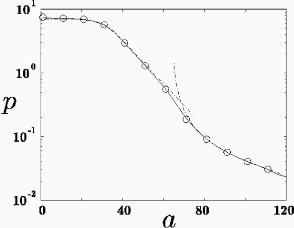
FIG. 3.: Static variational solution for $p$ as a function of $a$ (full line), analytic solutions in the large and small $p$ limit (dashed-dotted line), solution of the minimization of the exact Hamiltonian (circles). All results are for $N=200$ and $g=5$; $a$ parametrize the barrier (see Eq.(18) with $V_{0}=ab$ [28]).

Given the analytic espressions in Eqs.(V B,V B), we observe that the oscillation frequency for large $p$ coincides with the breathing frequency in the harmonic potential approximating the cosine potential, and the oscillation frequency for small $p$ corresponds to the revival time when the cosine potential is negligible (see Sec. VI A). Aware of the fact that it is not possible to define a transition point between the two regimes, being it a smooth transition, we still calculate the value of $p$ at which the two frequencies coincide, get $p=0.125$ and claim that the phase relation between the two condensates is smeared out for $p<0.125$.

VI Results: different regimes

In this section, we show some numerical results obtained by integrating the equations of motion for the variational parameters. In those results the full coupled dynamics of the process were considered. It is possible to compare with the evolution of the phase distribution governed by the Hamiltonian (82) with time–dependent coefficients. Moreover, it is possible to get analytic estimates concerning the typical time scales of the process.

In the three cases presented below we will fix the product $gN$ in order to have similar external dynamics and better isolate the effect of different $g$ and $N$ on the phase properties of the system. At the end of the process, when the barrier has reached its final value, depending on $N$ and $g$, one can have $gU_{1}\gg JN$ or $JN\gg gU_{1}$ (we assume that $U_{2}$ is then negligible). The case $gU_{1}\gg JN$ corresponds to the situation where the splitting process is completed and one expects a ground state with no well–defined relative phase. Instead in the case $JN\gg gU_{1}$ the ground state is still characterized by a localized phase distribution, and even if the two condensates are almost spatially separated they cannot be considered as independent. In this sense, the splitting is not complete.

A Complete splitting

We first analyse the case where in the final stage of the process, one has $gU_{1}\gg JN$. Since in this subsection and in the following we fix the product $gN$, this case is obtained for relatively small $N$ and large $g$. Depending on the time scale of the process, it is possible to observe collapses and revivals or to reach a final fragmented condensate characterized by very small number fluctuations.

We assume that in the final stage of the process it is possible to neglect $JN$ and $N^{2}U_{2}$, since they depend on the overlap of the two mode functions. Then the eingenstates are the number states

$${\hat{H}}|m\rangle=gU_{1}m^{2}|m\rangle.$$ (90)

and the time evolution of the final state corresponds to

$$|\Phi(t)\rangle\propto$$ (91)

$$\sum_{m}\exp\left(-\frac{m^{2}}{4p_{fin}}\right)\exp\left(-igU_{1}m^{2}t\right)|m\rangle.$$ (92)

In the variational ansatz formulation, one can plot the constant energy trajectories for the final barrier height (see Fig. 4(a)). Then, the time evolution corresponds to $p$ and $x_{I}$ following one of these trajectories: $p$ keeps almost constant and $x_{I}$ evolves unbounded increasing linearly with time with “velocity” $gU_{1}$ (see Eq.(89)), which exactly reproduces the phase in Eq.(91).

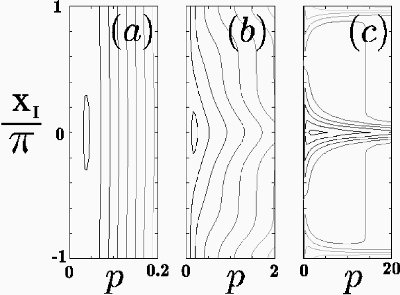
FIG. 4.: Contour plot of ${\cal H}$ for $a=120$: (a) $N=2\times 10^{3}$, $g=0.5$, (b) $N=2\times 10^{4}$, $g=0.05$ and (c) $N=2\times 10^{5}$, $g=0.005$ .

The main features of this time evolution are the following: the width of the number distribution is constant (determined by $p_{fin}$) and do not evolve in time; instead the phase distribution collapses and revives: an initial distribution peaked around zero smears out, revives around $\phi=\pi$ and so on. Defining the collapse time as the time $\tau_{c}$ when $\sigma_{\phi}\sim\pi$ and the revival time as the time $\tau_{r}$ when the original phase distribution is recovered shifted by $\pi$, one gets [3, 7].

$$\tau_{c} \sim \frac{2}{4p_{fin}gU_{1}}$$ (94)

$$\tau_{r} = \frac{\pi}{gU_{1}}.$$ (95)

The collapse time is governed by $p_{fin}$, which depends in general on the barrier raising process and on the parameters $g$ and $N$.

The final width of the number distribution obtained after the raising of the barrier is completed depends on the time scale of the process. This is just given by the value $p_{fin}$ at which the number fluctuations are frozen. To evaluated it, we claim that as long as $\omega_{p}>2\pi/\tau$ the number fluctuations follow the static solution, and when $\omega_{p}=2\pi/\tau$, they are frozen out to a final value $p_{fin}$. Setting $\omega_{p}=2\pi/\tau$ in Eq.(LABEL:omegaplp) and substituting in Eq.(84), one gets [29]

$$p_{fin} = \frac{N}{4}\frac{1}{2[2J-gNU_{2}+gN(U_{1}-2U_{2})]}\frac{2\pi}{\tau}\sim$$ (96)

$$\sim \frac{1}{8gU_{1}}\frac{2\pi}{\tau}.$$ (97)

Of course Eq.(96) is not valid for $\tau\rightarrow\infty$. For $\tau>2\pi/\ gU_{1}=2\tau_{r}$, we are in the adiabatic regime: $\omega_{p}>2\pi/\tau$ during all the process, and we expect to reach a completely delocalised relative phase.

We check this numerically and plot the results in Fig. 5 for several different splitting processes ($N=2\times 10^{2}$ and $N=2\times 10^{3}$). We actually find that for time scales $\tau>2\tau_{r}$ the final $p$ values lie in the region $p<0.125$. For faster time scales, the estimation in Eq.(96) was shown to be very good when the external degrees of freedom evolve adiabatically. Otherwise discrepancies can be observed (Fig. 5). It is not straighforward to estimate such discrepancies, since they depend on the exact dynamics and can be either positive or negative. Anyway, they are not striking and do not change from a situation in which the final relative phase is well defined to the opposite one.

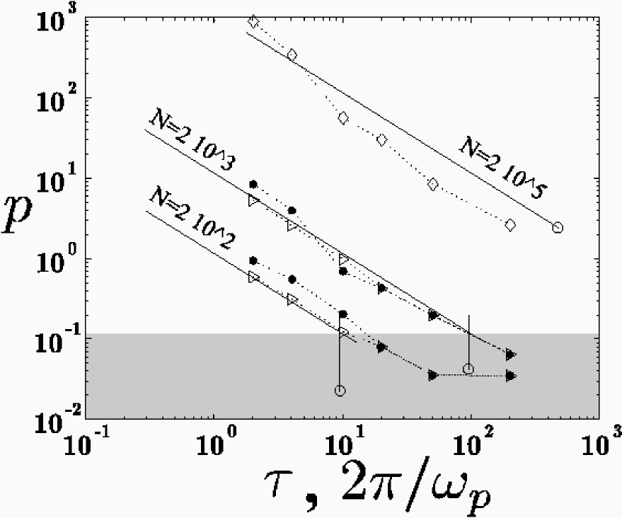
FIG. 5.: Case (i): $N=2\times 10^{2}$, $g=5$ and $N=2\times 10^{3}$, $g=0.5$. Final $p$ value against $\tau$: complete dynamics ($\bullet$) and adiabatic external dynamics ($\triangleright$); analytic solution for $p_{fin}$ against $2\pi/\omega_{p}$ in the large and small $p$ regimes (full lines); the shaded area is for $p\leq 0.125$ and represent the situation of completely delocalised relative phase; Case (ii): $N=2\times 10^{5}$, $g=0.005$; analytic solution for $p_{fin}$ (full lines) and numerical value for $p_{M}$ ($\diamond$); Static solutions for $a=120$ ($\circ$) [28]).

1 Collapses and revivals of the phase

Now we consider two of these splitting processes more in detail and compare quantitatively with the evolution of the phase distribution following the Hamiltonian in Eq.(82), where $J$, $U_{1}$ and $U_{2}$ vary in time with the barrier height according to the instantaneous static solution.

We have already mentioned that collapse and revival of the phase are predicted for two condensates with an initially good phase relation when the final tunneling coupling is negligible. Let us consider the case $N=2\times 10^{3}$, $g=0.5$ and $\tau=4$. In Fig. 6 we show the one-atom density matrix eigenvalues and the indetermination in the phase distribution $\sigma_{\phi}$. The agreement between the results of the two simulations is perfect [30] and our analytic estimations are also confirmed: we expect $\tau_{c}\sim 8$ and $\tau_{r}\sim 50$, which agree very well with the numerical results shown in Fig. 6.

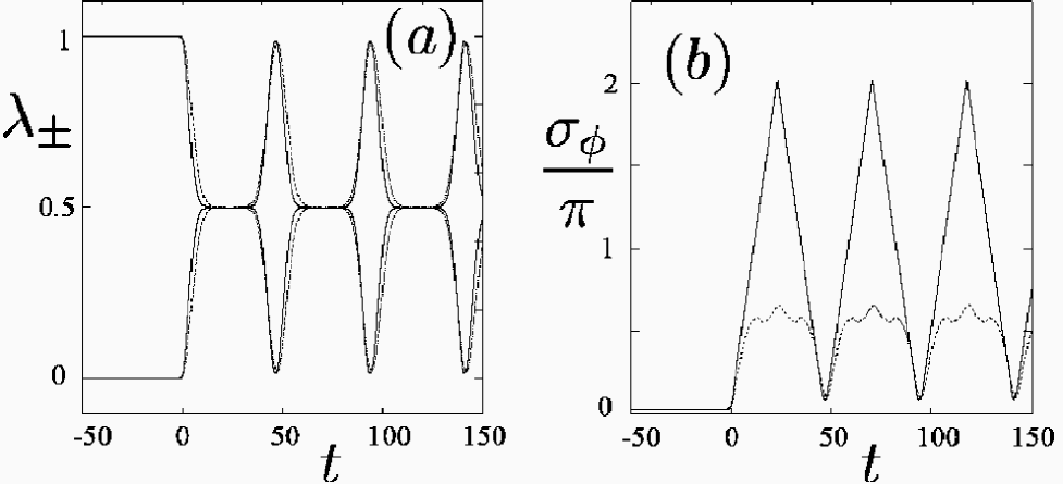
FIG. 6.: Eigenvalues $\lambda_{\pm}$ (a) and $\sigma_{\phi}/\pi$ (b). Numerical solutions for the variational ansatz (full line) and for the phase model (dotted line); $N=2\times 10^{3}$, $g=0.5$ and $\tau=4$.

The actual possibility of observing the revivals of the phase in an experiment is something outside our model. If they are actually destroyed by particles losses [24], one is left with two condensate with no phase relation, but higher number fluctations than they would have in the ground state.

2 Final fragmented condensate

Another way to cut the initial condensate into two independent ones, is to raise the barrier much slower, so that the phase coherence is lost adiabatically all along the process. So, we now choose again $N=2\times 10^{3}$, $g=0.5$ but a longer time scale $\tau=200$.

The agreement between the results of the variational ansatz and the phase model is very good also in this case. The final state is characterised by much smaller number fluctations with respect to the previous case (see Fig. 7(a)) and by a complete delocalised relative phase as shown in Fig. 7(b).

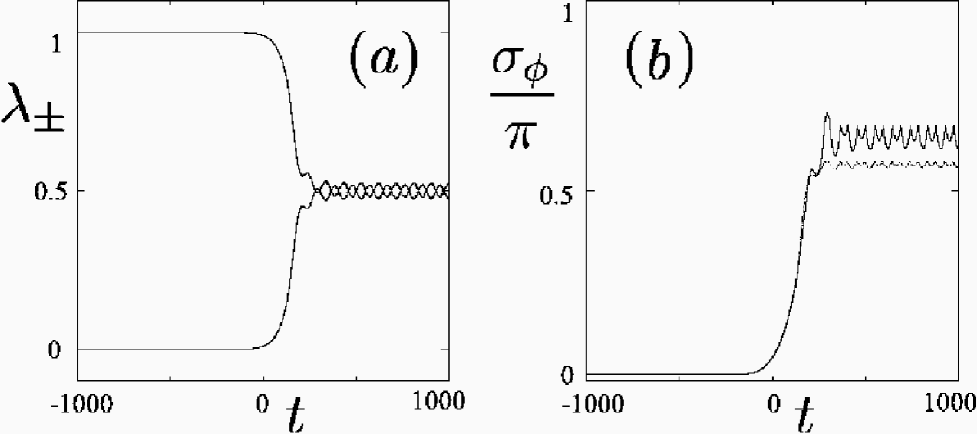
FIG. 7.: Eigenvalues $\lambda_{\pm}$ (a) and $\sigma_{\phi}/\pi$ (b). Numerical solutions for the variational ansatz (full line) and for the phase model (dotted line); $N=2\times 10^{3}$, $g=0.5$ and $\tau=200$.

From our analytic estimations, we actually expect to reach the static solution for $\tau>2\tau_{r}\sim 100$. Instead as it can be seen in Fig. 5 for $N=2\times 10^{3},\tau=200$, this does not happen. Dealing with such small values of $p_{fin}$ it is very easy to get at the end very small excitations, which can be due both to the external degrees of freedom or to some excitations already present in the initial conditions. The important feature is that the final relative phase is anyway completely delocalised.

B Incomplete splitting

We now analyse the case where in the final stage of the process, one has $JN\gg gU_{1}$. This case is obtained for large $N$ and small $g$: in the limit of large $N$, even if $J$ might be very small, it can happen that $JN>gU_{1}$ and the cosine potential in the phase representation (Eq.(82)) is not negligible. This can be seen as a process in which the barrier is raised up to a level at which the splitting is not really completed.

In the case in which the cosine potential at the end of the raising process is still deep, so that the lowest levels can be approximated with harmonic oscillator levels spaced by $\sqrt{2JNgU_{1}}$, the time evolution follows

$$|\Phi(t)\rangle\propto\sum_{n}c_{n}\exp\left(-in\sqrt{2JNgU_{1}}t\right)|n\rangle,$$ (98)

where $|n\rangle$ are the harmonic oscillator eigenstates and where the coefficients $c_{n}$ depend on the exact dynamics of the raising process. In particular, for symmetric initial conditions, the phase distribution is always symmetric and only the even eigenstates are populated. Then, the phase distribution breathes with a frequency $2\sqrt{2JNgU_{1}}$, remaining always centered at $\phi=0$. Moreover we notice that in such a case, the width in the number distribution is not expected to be constant. In the variational ansatz treatment, we have to look again at the orbits in the phase space. The contour plot in Fig. 4(b) is just to show how the orbit modify from the limit of small $N$ to the limit of large $N$. So let us consider Fig. 4(c). The orbits around the minimum of ${\cal H}$ represent a time evolution in which both the width of the number and phase distribution change in time. The frequency of the small oscillations around the equilibrium position can be calculted analytically for $\exp(-\sigma_{\phi}^{2}/2)\sim 1$ (see Eq.(LABEL:omegaplp) for $U_{2}=0$) and coincides with the breathing frequency of the phase distribution in the case of the superposition of harmonic oscillator eigenstates if $gNU_{1}\gg J$. If this condition is not satisifed, one is not in the weak coupling regime and the phase model is not valid.

The orbits in the $p$–$x_{I}$ space are characterised by very large oscillations in $p$. Hence we cannot talk of frozen number fluctations. Nevertheless, with arguments similar to the ones used before, we can try to identify the orbit which describes the dynamics at the end of the process. We estimate the maximum $p$ value in such an orbit to be $p_{M}\sim p_{fin}$. The agreement with the numerical solution can be checked in Fig. 5 and it is within a factor of $2$. The adiabaticity condition in this case consists in requiring that the final state is superfluid, as the static solution would be. This means that the minimum value of $p$ corresponding to the same orbit as $p_{M}$ must be such that the phase coherence is still good. We found that a final phase coherence corresponding to a minimum of $\lambda_{+}=1-\beta$ (with $\beta\ll 1/2$) is reached in process with typical time scales $\tau_{\beta}=2\pi/8JN\beta$. Note that this condition is weaker than requiring $p_{fin}=p_{s}$. In fact $\tau_{\beta}<\tau_{s}=2\pi/\sqrt{8NJgU_{1}}$, since $\beta<\sqrt{gU_{1}/8JN}$, as it would correspond to the static solution. This means that we still allow even big oscillation of $p$ around the equilibrium value, as long as they do not destroy the phase coherence. This corresponds to a breathing of the phase distribution which never becomes completely smeared out. Moreover, while $\tau_{s}$ depends only on the product $gN$, the adiabatic time scale $\tau_{\beta}$ scales like 1/N, getting easier and easier to be met for large $N$.

1 Final superfluid phase

As done before, we take now a particular case and check directly the results with the one obtained in the phase model. We choose $N=2\times 10^{5}$, $g=0.005$ and $\tau=50$ and find that the eigenvalues $\lambda_{\pm}$ oscillate with frequency $\omega_{p}$ (see Fig. 8(a)): $\lambda_{+}$ is always close to $1$ and $\lambda_{-}$ close to $0$. This corresponds to the breathing of the phase distribution in the non negligible cosine potential or in the variational ansatz treatment to one of the orbits in Fig. 4(c). No complete smearing out of the phase is observed (see Fig. 8(b)). Those results are confirmed up to a good level by the phase model (see Fig. 8(a,b)), even if the oscillations of $\sigma_{\phi}$ are damped, due to the anharmonicities of the cosine potential.

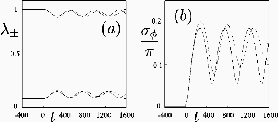
FIG. 8.: Eigenvalues $\lambda_{\pm}$ (a) and $\sigma_{\phi}/\pi$ (b). Numerical solutions for the variational ansatz (full line) and for the phase model (dotted line); $N=2\times 10^{5}$, $g=0.005$ and $\tau=50$.

The conditions that preserve the superfluid state are that the final tunneling coupling $JN$ is comparable to the on-site interaction and that the time scale of the process is slow enough to allow final small oscillations around the equilibrium. To destroy the phase coherence in this parameter range, one should raise the barrier faster in order to get larger oscillations, or raise it higher (case described in Sec. VI A).

To summarise, in this Section we have determined analytic expressions for the adiabaticity conditions for the internal dynamics, i.e. we identified the time scale at which the barrier can be raised in order to obtain the same relative phase properties as expected for the ground state. Concerning a completed splitting process, a fragmented condensate without any relative phase (no collapses and revivals) and characterised by a very narrow number distribution is reached in raising process with time scale $\tau>2\tau_{r}$. This means that the process has to be slower for large $N$ and small $g$. Instead in an incomplete splitting process, the superfluid phase is preserved for $\tau>2\pi/8JN\beta$. This time scale becomes shorter for large $N$. Both conclusions agree with the fact that in the Gross-Pitaevskii limit ($N\rightarrow\infty$ and $g\rightarrow 0$) the condensate is phase coherent.

VII Discussion and conclusions

We have solved the two-mode model describing the splitting of a condensate by a potential barrier through a variational ansatz. We found coupling between the internal and the external dynamics of the mode functions. We have identified the regimes in which the two dynamics decouple, and have concluded that in the case of splitting starting from a condensate in the ground state, they do not influence each other in a dramatic way. Hence, the internal and external excitations created by raising the barrier can be estimated in a good approximation independently and have been characterised as a function of the interaction strength, the number of atoms and the time scale of the process.

From our analytic estimations, confirmed by numerical resuts, we were able to identify the time scales $\tau_{z}$, $\tau_{p}$ and $\tau_{\beta}$, which define the adiabatic regime for the external and internal dynamics (respectively in the case of final fragmented or phase coherent condensate)

$$\tau_{z}\gg\frac{1}{\omega_{z}},\;\tau_{p}>2\tau_{r}=2\frac{\pi}{gU_{1}},\;\tau_{\beta}>\frac{2\pi}{8JN\beta}.$$ (99)

It is interesting to compare the adiabaticity condition for internal and external degress of freedom in the case of final fragmented condensate, when the splitting process can be consider to be completed. We normally found $\tau_{z}<\tau_{p}$; the case $N=200$, $g=5$ sets a boundary where internal and external degrees of freedom enter simultaneously the adiabatic regime for $\tau\sim 20$ (see Fig. 5). To get $\tau_{z}>\tau_{p}$ one needs $gU_{1}$ to be large compared to the trapping frequency. The quantity $gU_{1}$ is similar to the derivative of the chemical potential with respect to the total number of atoms $\partial\mu/\partial N$. From a Thomas-Fermi solution one gets that either in $1$ or $3$ dimensions, it scales as a negative power of $N$ and a positive power of $g$. So one needs to have very large $g$ or very small $N$, and our model fails in both limits. Therefore, we claim that in the usual regime of many weakly interacting particles, the adiabaticity condition for the phase dynamics is more restrictive than the one for the external dynamics.

We carried out a comparison of our model with the phase model, finding a substancial very good agreement. The numerical solution of the phase model consists in the integration of a time dependent Schrödinger equation. In practice, the number of wavefunctions $\varphi_{m}(\phi)=\exp(im\phi)/\sqrt{2\pi}$ that one has to use increases linearly with $N$, which leads to numerical problems. In this sense for large $N$, the variational ansatz is more convenient and has proved to give reliable results. Moreover the variational ansatz treatment allows to include the external degrees of freedom in a natural way.

In the previous results we did not take asymmetries into account. It is possible to include them in our ansatz, through the unbalance in population $m_{0}$ and through non symmetrically centered wave functions. In the case of complete splitting, one ends up with a final constant unbalance in population. The phase coherence shows the only new feature that the center of the phase distribution is now drifting with a velocity $\mu_{1}-\mu_{2}$, where $\mu_{i}$ are the chemical potentials of the two separate condensates. A complete analysis of this case, which even consideres losses and fluctuations in the total number of particles, can be found in [24]. Instead in the case of final phase coherent symmetric condensate, the asymmetry can destroy the phase coherence. The final unbalance in population might be so big, that the wavepacket describing the phase distribution flies above the cosine potential: depending on the “kinetic energy” $gU_{1}m_{0}^{2}$, the cosine potential may become negligible and the same features (collapses, revivals) as in the fragmented condensate case are observed.

Possible extensions of our model are the dynamic turning on of an optical lattice, where the initial harmonic trap is deformed into a many wells potential. The instantaneous version of such a process has recently been investigeted in [31]. Another problem of great significance is the inverse process, i.e. the merging of two condensates. This could allow to refill a condensate and be an important step towards a continuous atom laser.

A Two–mode variational ansatz approach and phase model

Dealing with two coupled condensates, in this paper we have often talked about the number difference $m$ and relative phase $\phi$. In this appendix, we will define number difference ${\hat{m}}$ and relative phase ${\hat{\phi}}$ operators, and derive the phase model Hamiltonian (82), discussing the approximations involved.

We first define the operators

$${\hat{L}}_{x} = \frac{1}{2}\left(a_{1}^{{\dagger}}a_{2}+a_{2}^{{\dagger}}a_{1}\right),$$ (A2)

$${\hat{L}}_{y} = \frac{i}{2}\left(a_{1}^{{\dagger}}a_{2}-a_{2}^{{\dagger}}a_{1}\right),$$ (A3)

$${\hat{L}}_{z} = \frac{1}{2}\left(a_{2}^{{\dagger}}a_{2}-a_{1}^{{\dagger}}a_{1}\right),$$ (A4)

such that the usual angular momentum commutation relations are fulfilled $[{\hat{L}}_{i},{\hat{L}}_{j}]=i\varepsilon_{ijk}{\hat{L}}_{k}$. After a small amount of algebra, the exact two–mode Hamiltonian in Eq.(79) can be rewritten as

$${\hat{H}}=g(U_{1}-2U_{2}){\hat{L}}_{z}^{2}-2J{\hat{L}_{x}}+gU_{2}\left({\hat{L}}_{x}^{2}-{\hat{L}}_{y}^{2}\right).$$ (A5)

In the subspace of fixed even total number of atoms $N$, the spectrum of ${\hat{L}}_{z}$ is given by all integer number in the interval $[-N/2,N/2]$. The operator ${\hat{L}}_{z}$ coincides with the number difference operator ${\hat{m}}$. We have often treated the eigenvalues $m$ as continuous, but in general care should be exercised. Given the phase operator ${\phi}$ such that $[{\hat{\phi}},{\hat{L}_{z}}]=i$, it is well–known that in the phase–representation ${\hat{L}}_{z}=\hat{m}=-i\partial/\partial\phi$ and the eigenstates of ${\hat{L}}_{z}$ ($\hat{m}$) with eigenvalue $m$ are $\langle\phi|m\rangle=\exp(im\phi)/\sqrt{2\pi}$ [26].

The state of the system $|\Phi\rangle$ can be in equivalent ways described as a superposition of eigenstates of ${\hat{m}}$ ($c_{m}$ is the number distribution)

$$|\Phi\rangle=\sum_{m=-N/2}^{N/2}c_{m}|m\rangle.$$ (A6)

or by a wave function in the $\phi$-representation given by

$$\Phi(\phi)=\langle\phi|\Phi\rangle=\frac{1}{\sqrt{2\pi}}\sum_{m=-N/2}^{N/2}c_{m}\exp(im\phi).$$ (A7)

Typical quantities characterizing $|\Phi\rangle$ are

- the width of the number distribution

$$\langle{\hat{m}}\rangle = \sum_{m}m|c_{m}|^{2},$$ (A8)

$$\sigma^{2}_{m} = \sum_{m}m^{2}|c_{m}|^{2}-\langle{\hat{m}}\rangle^{2};$$ (A9)

- the width of the phase distribution

$$\langle{\hat{\phi}}\rangle = \int_{-\pi}^{\pi}d\phi\,\phi\left|\Phi(\phi)\right|^{2},$$ (A10)

$$\sigma^{2}_{\phi} = \int_{-\pi}^{\pi}d\phi\,\phi^{2}\left|\Phi(\phi)\right|^{2}-\langle{\hat{\phi}}\rangle^{2}$$ (A11)

The uncertainty relations are the same one as for angular momenta [26].

In order to write the Hamiltonian in the phase–representation, we make some approximations which will lead to the simple phase model Hamiltonian and discuss under which conditions such approximations are valid. We will describe the procedure only for the term ${\hat{L}}_{x}$, since for the term ${\hat{L}}_{x}^{2}-{\hat{L}}_{y}^{2}$ an analogous one applies. Using the raising and lowering operators ${\hat{L}}_{\pm}$, we write

$$\langle\phi|2{\hat{L}}_{x}|\Phi\rangle=\sum_{m}c_{m}\langle\phi|\left({\hat{L}}_{+}+{\hat{L}}_{-}\right)|m\rangle=$$ (A12)

$$=\frac{N+1}{\sqrt{2\pi}}\sum_{m}c_{m}\frac{1}{2}e^{im\phi}$$ (A13)

$$\left[\sqrt{1-\left(\frac{2m+1}{N+1}\right)^{2}}e^{i\phi}+\sqrt{1-\left(\frac{2m-1}{N+1}\right)^{2}}e^{-i\phi}\right].$$ (A14)

We assume a narrow and centered number distribution (these assumptions will be quantified later on), so that we can expand the square roots at first order in $(m/N)^{2}$ and get

$$\langle\phi|2{\hat{L}}_{x}|\Phi\rangle=$$ (A15)

$$=(N+1)\cos\phi\Phi(\phi)+$$ (A16)

$$+2(N+1)\left[\frac{{\widetilde{m^{2}}}+1/4}{(N+1)^{2}}\cos\phi+\frac{{\tilde{m}}}{(N+1)^{2}}\sin\phi\right]+$$ (A17)

$$+o\left(\frac{{\widetilde{m^{4}}}}{N^{4}}\right)\approx N\cos\phi\;\Phi(\phi),$$ (A18)

where we can roughly estimate

$$\left|{\widetilde{m^{2}}}\right|^{2}\equiv\left|\sum_{m}c_{m}m^{2}\langle\phi|m\rangle\right|^{2}<$$ (A19)

$$<\left|\sum_{m}|c_{m}|m^{2}m^{2}\right|^{2}\leq\sum_{m}|c_{m}|^{2}m^{2}\sum_{m^{\prime}}m^{\prime 2}=$$ (A20)

$$=\left(\sigma_{m}^{2}+\langle m\rangle^{2}\right)\sum_{m=\langle m\rangle-\sigma_{m}}^{\langle m\rangle+\sigma_{m}}m^{2}\sim\left(\sigma_{m}^{2}+\langle m\rangle^{2}\right)^{2}\sigma_{m}<$$ (A21)

$$<\left(\sigma_{m}+|\langle m\rangle|\right)^{4}\sigma_{m},$$ (A22)

so that $\left|\widetilde{m^{2}}\right|<(\sigma_{m}+|\langle m\rangle|)^{2}\sqrt{\sigma_{m}}$ and where in a similar way $|{\tilde{m}}|\equiv\left|\sum_{m}c_{m}m\langle\phi|m\rangle\right|\sim(\sigma_{m}+|\langle m\rangle|)\sqrt{\sigma_{m}}$. In an analogous way, the term ${\hat{L}}_{x}^{2}-{\hat{L}}_{y}^{2}$ gives

$$4\left({\hat{L}}_{x}^{2}-{\hat{L}}_{y}^{2}\right)\approx$$ (A23)

$$\approx N^{2}\cos 2\phi-4\left[(\widetilde{m^{2}}+1)\cos 2\phi+2{\tilde{m}}\sin 2\phi\right]\approx$$ (A24)

$$\approx N^{2}\cos 2\phi.$$ (A25)

All together the neglected terms have to be smaller than all the other terms in the Hamiltonian, which implies

$$\left|\widetilde{m^{2}}\right|\sim\left(\sigma_{m}+|\langle m\rangle|\right)^{2}\sqrt{\sigma_{m}}\ll N^{2}$$ (A26)

$$\frac{2J-gNU_{2}}{N}\ll g(U_{1}-2U_{2}).$$ (A27)

For $|\langle m\rangle|\ll\sigma_{m}$, which is the typical situation treated in this paper, from the first equation one gets $\sigma_{m}\ll N^{4/5}$. In the opposite limit where $|\langle m\rangle|\gg\sigma_{m}$ instead one has

$$\frac{|\langle m\rangle|}{N}\ll\frac{1}{\sigma_{m}^{1/4}}.$$ (A28)

For $\sigma_{m}\rightarrow 0$ this condition is not correct and becomes simply $|\langle m\rangle|\ll N$.

To summarise, in the specific case treated in this paper, where no unbalance of population between the wells was assumed, the important condition of validity for the phase model Hamiltonian is Eq.(A27), which written for $U_{2}=0$ takes the form

$$J\ll gNU_{1}/2.$$ (A29)

We note that under such a condition, the ground state is characterised by $\sigma_{\phi}\gtrsim\sqrt{1/N}$ or equivalently $\sigma_{m}\lesssim\sqrt{N/4}$.

B Comparison between variational ansatz and phase model

In this subsection we will compare the phase model with our variational ansatz. For simplicity we set $U_{2}=0$, but the following discussion could be repeated in the more general case. In particular for $U_{2}=0$ the phase model Hamiltonian reduces to the Josephson Hamiltonian [21]

$${\hat{H}}=-gU_{1}\frac{\partial^{2}}{\partial\phi^{2}}-JN\cos\phi.$$ (B1)

The quantities $gU_{1}$ and $JN$ are respectively the on-site energy splitting (charging energy) and the tunneling coupling (Josephson coupling). It describe accurately the case of high barrier, where the two condensates are almost spatially separated, leading to a negligible $U_{2}$, and are characterised by very small number fluctuations, making the Josephson Hamiltonian valid. The phase model Hamiltonian in Eq.(B1) describes the motion of a particle in a cosine potential and the classical limit is obtained for $\sigma_{m},\sigma_{\phi}\rightarrow 0$. In the following we discuss the classical and quantum limits comparing it directly with the variational ansatz results.

In order to allow a complete comparison with the Hamiltonian in Eq.(B1), we now describe the coefficients $c_{m}$ in Eq.(3) with four variational parameters $p$, $x_{I}$, $m_{0}$ and $\varphi$

$$c_{m}=$$ (B2)

$${\cal N}(p)\exp\left[-\left(\frac{1}{4{p}}+i{x_{I}}\right)(m-m_{0})^{2}\right]\exp[im\varphi],$$ (B3)

The variational parameters $x_{I}$ and $\varphi$ are the variables conjugate to $p$ and $m_{0}$, allow the dynamic evolution and vanish in the ground state. In the limit of broad number distribution this ansatz describes a gaussian superposition of number states centered in $m=m_{0}$. The corresponding phase distribution $\Phi(\phi)$ is also a gaussian, centered in $\phi=\varphi$. Notice that in the case of symmetric splitting treated before $m_{0}=0$ and $\varphi=0$ $\forall t$.

Replacing again the sum over $m$ from $-N/2$ to $N/2$ with an integral from $-\infty$ to $\infty$ (for $p\gtrsim 1$ and $x_{I}$ such that $\sigma_{\phi}\lesssim\pi$), the widths of the number and phase distribution are respectively given by Eqs.(III D) and the expectation values $\langle a_{i}^{{\dagger}}a_{j}\rangle$ and $\langle a_{i}^{{\dagger}2}a_{i}^{2}\rangle$ on the state $|\Phi\rangle$ are now

$$\langle\Phi|a_{1,2}^{{\dagger}}a_{1,2}|\Phi\rangle=\frac{N}{2}\mp m_{0},$$ (B5)

$$\langle\Phi|a_{1,2}^{{\dagger}2}a_{1,2}^{2}|\Phi\rangle=\frac{N^{2}}{4}+p\mp Nm_{0}+m_{0}^{2},$$ (B6)

$$\langle\Phi|a_{1}^{{\dagger}}a_{2}|\Phi\rangle=\langle\Phi|a_{2}^{{\dagger}}a_{1}|\Phi\rangle^{*}=$$ (B7)

$$=\frac{N}{2}\exp\left(-\frac{\sigma_{\phi}^{2}}{2}\right)\exp\left(i\varphi\right)$$ (B8)

$$\hskip 56.9055pt\left[1-\frac{2p}{N^{2}}+\frac{2}{N^{2}}\left(m_{0}-i2px_{I}\right)^{2}\right].$$ (B9)

a Classical limit

Let us first consider the classical limit and compare the results obtained with the variational ansatz with the phase model. We write the expectation value of the Hamiltonian (Eq.(79)) for $U_{2}=0$ in the classical limit by setting $\sigma_{m}=0$ and $\sigma_{\phi}=0$

$${\cal H}_{cl}=gU_{1}m_{0}^{2}-JNcos\varphi;$$ (B10)

here we have assumed $m_{0}\ll N$, neglected all terms $o(1/N)\ll 1$ and all terms independent of $m_{0}$ and $\varphi$. One sees immediately that this expression coincide with the Hamiltonian in Eq.(B1), where the operators have been substituted with their expectation values ($\langle{\hat{m}}\rangle=m_{0}$ and $\langle{\hat{\phi}}\rangle=\varphi$). So, the analogy with the phase model in the classical limit is straighforward [10]. In particular if $J>0$ the stable equilibrium position is $\phi=0$; for a kinetic energy such that $gU_{1}m_{0}^{2}<JN$ the phase undergoes oscillations, otherwise if $gU_{1}m_{0}^{2}>JN$ the phase flies above the cosine potential.

b Quantum limit

In the quantum limit the width of the number and phase distribution start to play an important role. The comparison between the two models now is not so trivial, because we have on the one hand a wavefunction in the phase representation, $\Phi(\phi)$, and on the other hand $4$ variational parameters ($p$, $x_{I}$, $m_{0}$ and $\varphi$) which follow a classical dynamics and should reproduce the features of $\Phi(\phi)$. We consider here the simplified case of a wavefunction $\Phi(\phi)$ symmetric around $\phi=0$. In the variational ansatz picture, this corresponds to $m_{0}=$ and $\varphi=0$ $\forall t$. This last assumption is correct for symmetric initial conditions and preserved at all times, how can be checked esplicitly in the equations of motion.

Concerning the ground state of Hamiltonian (B1), two different regimes can be identified: for $gU_{1}\gg JN$, the cosine potential can be neglected and the ground state is a flat wavefunction, which corresponds to a completely undefined relative phase between the two condensates. Instead for $gU_{1}\ll JN$ the cosine potential is deep and the ground state is a localised wavefunction, which describe a state with very well defined relative phase. In the variational ansatz approach, to find the ground state we set $x_{I}=0$, $m_{0}=0$ and $\varphi=0$, and get ${\cal H}(p)=gU_{1}p-JN\exp(-1/8p)\left[1-2p/N^{2}\right]$. For $gU_{1}\ll JN$, the minimum of this Hamiltonian is $p=N/4$ corresponding to the Gross-Pitaevkii limit ($\sigma_{\phi}\sim 1/\sqrt{N}$) and if the hopping decreases $p\rightarrow 0$ ($\sigma_{\phi}\gg\pi$), reproducing the same results as the phase model. A quantitative comparison shows perfect agreement.

The time evolution was discussed already in Sec. VI, where the analogy between the evolution of the phase distribution $\Phi(\phi)$ and the evolution of the variational parameters $p$ and $x_{I}$ was carried out. The variational ansatz is able to predict all the main features typical of the evolution of the phase distribution: collapses and revivals of the relative phase for $gU_{1}\gg JN$ and breathing of the wavefunction in the cosine potential for $JN\gg gU_{1}$. Moreover the frequency of the small oscillations around the equilibrium point calculated in the variational approach concides with the splitting of the energy levels of the phase model Hamiltonian both in the limit of negligible cosine potential and in the limit of deep cosine potential.

In this Appendix we have qualitatively compared the phase distribution described by the phase model with the Gaussian ansatz for the coefficients of the state $|\phi\rangle$ in the number representation. We have shown that in the classical limit the expectation values $m_{0}$ and $\varphi$ of number and phase (variational parameters indicating the centers of the respective Gaussian distributions) are governed by the classical phase model Hamiltonian. Moreover in the quantum description the parameters $p$ and $x_{I}$, related to the widths $\sigma_{m}$ and $\sigma_{\phi}$, are able to reproduce the same features of the time evolution predicted by the phase model, whose limit of validity of the phase model (derived in App. A) is $J\ll gU_{1}N/2$.

We discussed the limit of fragmented condensate ($JN\ll gU_{1}$) and the limit of single phase coherent condensate ($JN\gg gU_{1}$). As already mentioned, for fixed $gN$, the limit $N\rightarrow\infty$ corresponds to the Gross-Pitaevkii limit. Infact, unless $J=0$, if $N\rightarrow\infty$ the condensate is always phase coherent. For finite $N$, the above discussion allows to judge whether the Gross-Pitaevskii description is still valid or not.

REFERENCES

- [1] E. M. Wright and D. F. Walls, J. C. Garrison, Phys. Rev. Lett, 77, 2158 (1996)
- [2] M. Lewenstein and L. You, Phys. Rev. Lett. 77, 3489 (1996)
- [3] P. Villain, M. Lewenstein, R. Dum, Y. Castin, L. You, A. Imamoglu and T. A. B. Kennedy, Jour. of Mod. Opt. bf 44 1775-1799 (1997)
- [4] A. Sinatra and Y. Castin, Eur. Phys. J. D 8, 319 (2000)
- [5] C. K. Law, H. Pu, N. P. Bigelow and J. H. Eberly, Phys. Rev. A, 58, 531 (1998)
- [6] D. Jaksch, C. Bruder, J. I. Cirac, C. W. Gardiner and P. Zoller, Phys. Rev. Lett. 81, 3108 (1999)
- [7] G. J. Milburn and J. Corney, E. M. Wright, D. F. Walls, Phys. Rev. A, 55, 4318 (1997)
- [8] A. Smerzi, S. Fantoni, S. Giovanazzi and S. R. Shenoy, Phys. Rev. Lett. 79, 4950 (1997)
- [9] I. Zapata and F. Sols, A. J. Leggett, Phys. Rev. A, 57, R28 (1998)
- [10] A. Smerzi and S. Raghavan, cond-mat/9905059
- [11] J. Javanainen and M. Wilkens, Phys. Rev. Lett. 78, 4675 (1997)
- [12] A. J. Leggett and F. Sols, Phys. Rev. Lett. 81, 1344 (1998)
- [13] J. Javanainen and M. Wilkens, Phys. Rev. Lett. 81, 1345 (1998)
- [14] K. Mølmer, Phys. Rev. A 58, 566 (1998)
- [15] D. S. Rokhsar, cond-mat/9812260
- [16] J. Javanainen and M. Yu. Ivanov, Phys. Rev. A, 60, 2351 (1999)
- [17] K. Berg-Sørensen and K. Mølmer, Phys. Rev. A 58, 1480 (1998)
- [18] W. Ketterle, D. S. Durfee and D. M. Stamper-Kurn, Proceedings of the International School of Physics “Enrico Fermi”, Course CXL, M. Inguscio, S. Stringari and C. Wieman (Eds.), IOS Press, Amsterdam 1999
- [19] B. P. Anderson and M. A. Kasevich, Science, 82 1686 (1998)
- [20] V. M. Perez-García, H. Michinel, J. I. Cirac, M. Lewenstein and P. Zoller, Phys. Rev. Lett. 77, 5320 (1996)
- [21] A. J. Leggett and F. Sols, Found. Phys. 21, 353 (1991)
- [22] F. Sols, Physica B 194-196, 1389 (1994)
- [23] I. Carusotto, Y. Castin and J. Dalibard, cond-mat/0003399
- [24] A. Sinatra and Y. Castin, Eur. Phys. J. D 4, 247 (1998)
- [25] Eugen Šimánec, Inhomogeneous Superconductors. Granular and Quantum effects (Oxford Univ. Press, New York, 1994)
- [26] Quantum Mechanics I, A. Galindo P. Pascual, pp.201-204 and discussion in [4]
- [27] The definitions in Eqs.(74,76) are not general: they are valid always is the static case when are real and are always true in the specific case of our variational ansatz (see Eq.(13))
- [28] We will make the following choice with , so that the potential wells keep as symmetric as possible when varies. This leads to oscillation frequencies of the same order of magnitude at the beginning and at the end of the splitting process.
- [29] This conclusion is similar to the result in [16]. It is difficult to make a direct comparison between the two, since due to the more complex spatial and time dependence our tunneling rate does not decrease following a simple exponential.
- [30] In Fig. 6,7 (b) the values for do not coincide for , because we used Eq.(55) without correcting it, but they both indicate a complete smearing out of the relative phase.
- [31] J. Javanainen, Phys. Rev. A, 60, 4902 (1999)