Scale Invariance in the Nonstationarity of Physiological Signals

Abstract

We introduce a segmentation algorithm to probe temporal organization of heterogeneities in human heartbeat interval time series. We find that the lengths of segments with different local values of heart rates follow a power-law distribution. This scale-invariant structure is not a simple consequence of the long-range correlations present in the data. We also find that the differences in mean heart rates between consecutive segments display a common functional form, but with different parameters for healthy individuals and for patients with heart failure. This finding may provide information into the way heart rate variability is reduced in cardiac disease.

A time series is stationary if the mean, standard deviation and all higher moments, as well as the correlation functions, are invariant under time translation [1]. Signals that do not obey these conditions are nonstationary. Nonstationarity is a prominent feature of biological variability that can be associated with regimes (segments) of different statistical properties. The borders between different segments can be gradual or abrupt (Fig. 1).

A major problem in contemporary physiology is the presence of nonstationarity in time series generated under free-running conditions [2]. Physiological signals obtained under widely-varying conditions raise serious challenges to both technical and fundamental aspects of time series analysis. By filtering out effects of nonstationarity, much work has focused on “intrinsic properties” of physiological signals [3]. This approach is based on the implicit assumption that the nonstationarity arises simply from changes in environmental conditions — e.g., different daily activities — so environmental “noise” could be treated as a “trend” and distinguished from the more subtle fluctuations that may reveal intrinsic correlation properties of the dynamics. Indeed, important scale-invariant features in physiological processes were recently revealed after filtering out masking effects of nonstationarity [4]. However, nonstationarity itself is also an important feature of physiological time series and is known to change from healthy to pathological conditions [5], suggesting more than only enviromental conditions are reflected in the phenomena. Thus one would expect that there is a non-trivial structure associated with the nonstationarity in physiological signals, which may change with disease. To test this hypothesis we focus on one statistical property, the mean heart rate, which is related to physiologic responses and is commonly used for medical evaluation.

The problem is to partition a nonstationary time series, which is composed of many segments with different mean value, in such a way as to maximize the difference in the mean values between adjacent segments. We apply the following procedure: we move a sliding pointer from left to right along the signal. At each position of the pointer, we compute the mean of the subset of the signal to the left of the pointer ($\mu_{\rm left}$) and to the right ($\mu_{\rm right}$). To measure the difference between $\mu_{\rm left}$ and $\mu_{\rm right}$, we compute the t-statistic [6]:

$$t\equiv\left|\frac{\mu_{\rm left}-\mu_{\rm right}}{s_{D}}\right|$$ (1)

where $s_{D}$ is the pooled variance [7].

We next determine the position of the pointer for which $t$ reaches its maximum value, $t_{\rm max}$, and compute the statistical significance of $t_{\rm max}$ [8]. We check if this significance exceeds a given threshold ${\cal P}_{0}$. If so, then the signal is cut at this point into two subsequences; otherwise the signal remains undivided. If the sequence is cut, the procedure continues recursively for each of the two resulting subsequences created by each cut. Before a new cut is accepted, we also compute $t$ between the right-hand new segment and its right neighbor (obtained by a previous cut) and the $t$ between the left-hand new segment and its left neighbor (also obtained by a previous cut) and check if both values of $t$ have a statistical significance exceeding ${\cal P}_{0}$. If so, we proceed with the new cut; otherwise we do not cut. This ensures that all resulting segments have a statistically significant difference in their means. The process stops when none of the possible cutting points has a significance exceeding ${\cal P}_{0}$, and we say that the signal has been segmented at the “significance level ${\cal P}_{0}$” (Fig. 2).

Our method leads to partitioning of a time series into segments with well-defined means, each significantly different from the mean of the adjacent segments (Fig. 1). This allows us to probe the nonstationarity in a signal through the statistical analysis of the properties of the segments.

Here we consider 47 datasets from 18 healthy subjects, 17 records of cosmonauts during orbital flight and 12 patients with congestive heart failure [9]. We separately analyze 6–hour long subsets of each dataset, corresponding to the periods when the subject is awake or sleeping. Figure 1 shows a representative dataset of a healthy subject, and a subject with heart failure. Superposed on the interbeat interval series, we also plot the segments obtained by means of our segmentation algorithm.

To quantify the nonstationarity in heart rate variability, we study the statistical properties of the segments corresponding to parts of the signal with significantly different mean values. To characterize the segments, we analyze two quantities: (i) the length of the segments; (ii) the absolute values of the differences between the mean values of consecutive segments, which we call jumps.

(i) Distribution of segment lengths — Healthy subjects typically exhibit nonstationary behavior associated with large variability, trends, and segments with large differences in their mean values, while data from heart failure subjects are characterized by reduced variability and appear to be more homogeneous (Fig. 1) [5]. Thus, one might naively expect that signals from healthy subjects will be characterized by a large number of segments, while signals from heart failure subjects will exhibit a smaller number of segments (i.e., the average length of the segments for healthy subjects could be expected to be smaller than for heart failure subjects).

To test this hypothesis, we apply the segmentation algorithm to 6–hour records of interbeat intervals during daily activity, and find that for each healthy subject the distribution of segment lengths is well described by a power law with an identical exponent, indicating absence of a characteristic length for the segments. Surprisingly, we find that this power law remains unchanged for records obtained from cosmonauts during orbital flight (under conditions of microgravity) and for patients with heart failure (Fig. 3). A similar common type of behavior is also observed from 6–hour records during sleep for all three groups [10].

To verify the results of the segmentation procedure, we perform several tests. First, we check the validity of the observed power law in the distribution of segment lengths. We generate a surrogate signal formed by joining segments of white noise with standard deviation $\sigma=0.5$, and mean values chosen randomly from the interval $[0,1]$. We choose the lengths of these segments from a power-law distribution with a given exponent. Even when the difference between the mean values of adjacent segments is smaller than the standard deviation of the noise inside the segments, we find that our procedure partitions the surrogate signal into segments with lengths that reproduce the original power-law distribution [Fig. 4(a)]. This test shows that the distributions obtained after segmenting surrogate data with similar values of their exponents, appear clearly different from each other, making more plausible that the distributions obtained for the lengths of the segments for the healthy, cosmonauts and congestive heart failure subjects (Fig.3) follow indeed an identical distribution.

Second, we test if the observed power-law distribution for the segment lengths is simply due to the known presence of long-range correlations in the heartbeat interval series [11]. For that, we generate correlated linear noise [12] with the same correlation exponent as the heartbeat data. We find that the distribution of segment lengths obtained for the linear noise differs from the distribution obtained for the heartbeat data [Fig. 4(b)]. For the noise, the distribution decays faster, which means that these signals are more segmented than the heart data. In fact, for different linear noises with a broad range of correlation exponents, we do not find power-law behavior in the distribution of the segments. Thus we conclude that the linear correlations are not sufficient to explain the power-law distribution of segment lengths in the heartbeat data.

(ii) Differences between the mean values of consecutive segments (jumps) — Different healthy records can be characterized by different overall variance, depending on the activity and the individual characteristics of the subjects. Moreover, subjects with heart failure exhibit interbeat intervals with lower mean and reduced beat-to-beat variability (lower standard deviation). Thus one can trivially assume that these larger jumps in healthy records are due only to the fact that their average standard deviation is larger [Fig. 1(a)(b)]. In order to systematically compare the statistical properties of the jumps between different individuals and different groups, we normalize each time series by subtracting the global average (over 6 hours) and dividing by the global standard deviation. In this way, all individual time series have zero mean and unit standard deviation [Fig. 1(c)(d)]. Such a normalization does not affect the results of our segmentation procedure.

We find that both the healthy subjects and the cosmonauts follow identical distributions, but the distribution of the jumps obtained from the heart failure group are markedly different — centered around lower values — indicating that, even after normalization, there is a higher probability for smaller jumps compared to the healthy subjects [Fig. 5(a)]. Note that the distributions for all groups appear to follow an identical homogeneous functional form, so we can collapse these distributions on top of each other by means of a homogeneous transformation [Fig. 5(b)]. The ratio between the scaling parameters used in this transformation gives us a factor by which this feature of the heartrate variability is reduced for the subjects with heart failure as compared to the healthy subjects. This finding indicates that, although the heartrate variability is reduced with disease, there may be a common structure to this variability, reflected in the identical functional form. These observations agree with previously reported results for the distribution of heartbeat fluctuations obtained by means of wavelet and Hilbert transforms [13].

In summary, we present a new method to probe the nonstationarity of a signal by partitioning it into segments with different mean values. We find a scale-invariant structure in the nonstationarity of a time series representative of a complex dynamics, namely the human heartbeat. This structure is characterized by a power-law distribution of the lengths of segments with a scaling exponent which does not change under certain pathological conditions and cannot be explained by the presence of correlations in the data. We find also a common structure to the jumps between consecutive segments, with a change in the scaling parameters with disease.

We thank Y. Ashkenazy, V. Schulte-Frohlinde, I. Grosse, S. Havlin, S. Mossa, C.-K. Peng, and Z. Struzik for helpful discussions and suggestions, grants BIO99-0651-CO2-01 (from the Spanish Government) and NIH/NCRR (P41RR13622), NASA, and the Mathers Charitable Foundation for support.

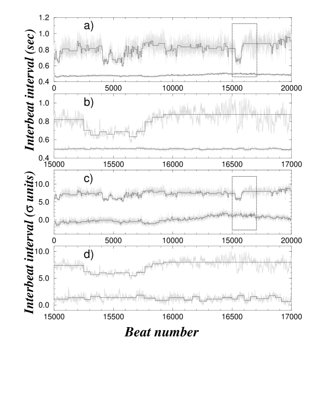
FIG. 1.: (a) Plot of 20,000 interbeat intervals ($\approx$ 6 hours) for a healthy subject (upper curve) and a subject with heart failure (bottom curve). Note the larger variability and patchiness for the healthy record. (b) Magnification of a small fraction (2000 beats) of the signals in (a). (c) Same signals as displayed in (a) after subtracting the global average and dividing by the global standard deviation; after this normalization both signals appear very similar. (d) Magnification of a small fraction (2000 beats) of the signals in (c).

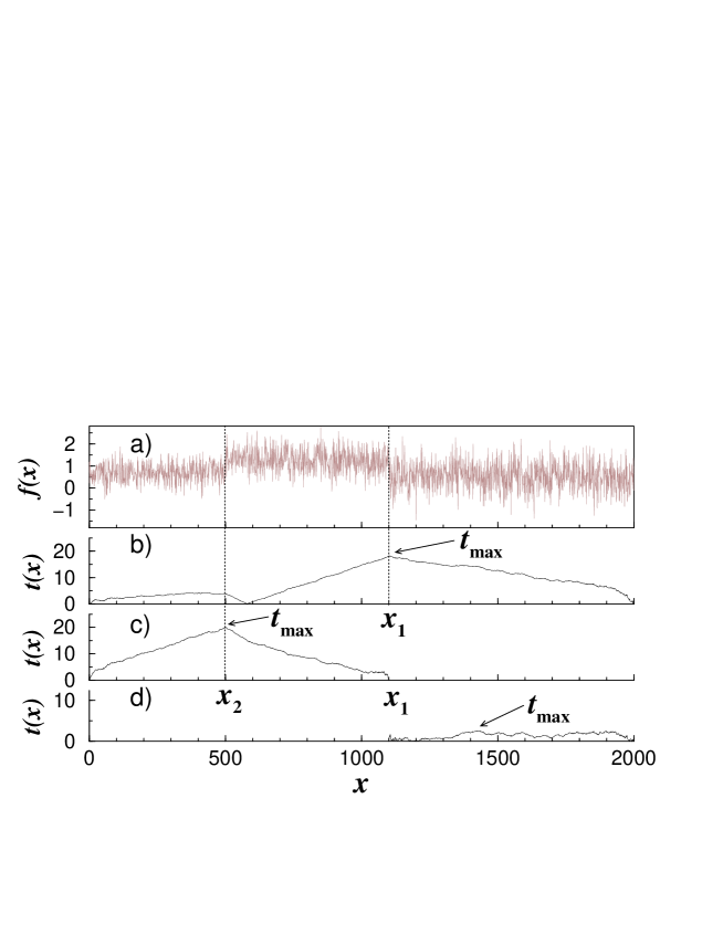
FIG. 2.: (a) An artificial time series $f(x)$ composed of three segments with different mean values. (b) Values of the statistic $t$, defined in Eq. (1), obtained by moving the pointer along the time series. Note that $t_{\rm max}$ is reached at $x_{1}$. We find that if ${\cal P}(t_{\rm max})\geq{\cal P}_{0}=95\%$, and so we cut the series at $x_{1}$. (c) We iterate the procedure with the segment $[0,x_{1}]$. We find that ${\cal P}(t_{\rm max})\geq 95\%$ and we also find that the significance of $t$ computed between $[x_{2},x_{1}]$ and $[x_{2},2000]$ is greater than $95\%$, so the series is cut at $x_{2}$. (d) We iterate the procedure with the segment $[x_{1},2000]$. Now, ${\cal P}(t_{\rm max})\leq 95\%$, so this segment is not cut.

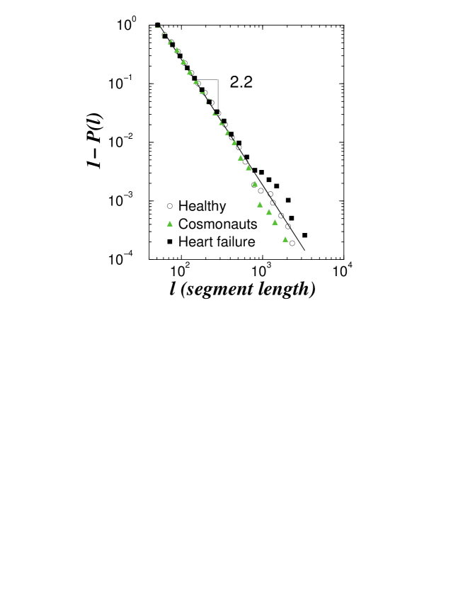
FIG. 3.: Probability of finding segments with a length $\ell$ larger than a given value for the segments obtained from all subjects in the healthy, cosmonauts and heart failure groups during during daily activity. The significance level is fixed to ${\cal P}_{0}=95\%$, and the imposed minimum length of the segments is $\ell_{0}=50$ beats. For all three groups we find a power law in the distribution of segment lengths with exponent $\beta\approx 2.2$, and we find that $\beta$ depends on $\ell_{0}$ and on ${\cal P}_{0}$. For all $\ell_{0}$ and ${\cal P}_{0}$, the value of $\beta$ is the same for each three groups.

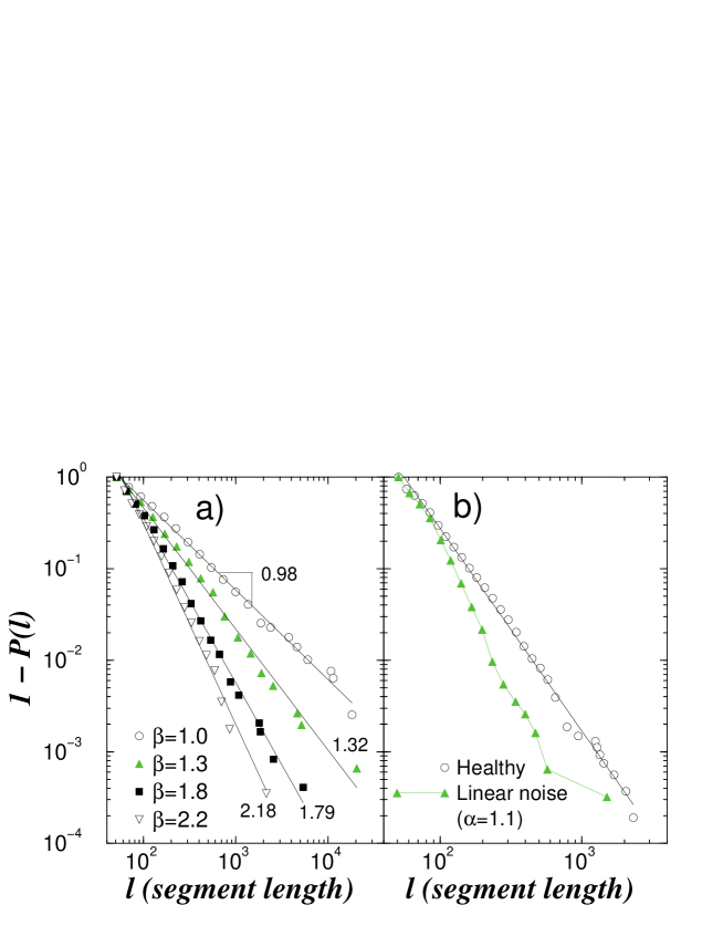
FIG. 4.: (a) Testing the validity of the observed power-law behavior in the distribution of segment lengths. We generate a surrogate signal formed by joining segments of white noise with standard deviation $\sigma=0.5$ and average values chosen randomly from the interval $[0,1]$. We chose the lengths of these segments from a power-law distribution with a given exponent $\beta$. The test shows that the distributions obtained after segmenting the surrogate data generated from power-law distributions with nearby values of their exponents appear clearly separated. This suggests that the distributions for the healthy, cosmonauts and congestive heart failure subjects in Fig. 3 are indeed identical. (b) Testing the effect of correlations in the heartbeat fluctuations on the segmentation. We generate 10 realizations, each with length of 26,000 points, of a linear Gaussian-distributed correlated noise with an exponent $\alpha=1.1$ [12]. This exponent is calculated using the detrended fluctuation analysis method and is identical to the exponent $\alpha$ observed for the heartbeat data [11]. The distribution of segment lengths for this correlated noise does not follow the power law found for the heartbeat data. This test suggests that the observed scale-invariant behavior in the distributions of segment lengths in the heartbeat is not simply due to the correlations. According to the results in (a), the differences found between heartbeat data and correlated noise are significant. To verify that the curvature found in the distribution of segments for the noise is not due to finite size effects, we also repeated the test with longer realizations of the noise (1,000,000).

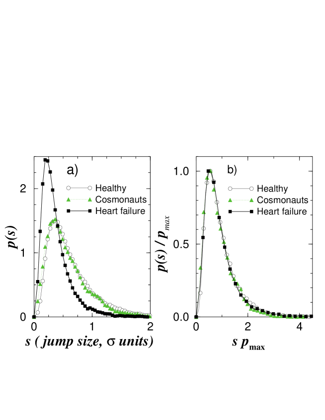
FIG. 5.: (a) Probability distribution of the absolute value of the difference between the mean values (‘jumps’) of consecutive segments. Both healthy and cosmonaut subjects follow an identical distribution while the heart-failure subjects follow a quite different distribution with higher probability for small jumps consistent with reports of smaller variability in heart failure subjects [5]. All distributions are normalized to unit area. (b) Same probability distributions as in (a), after rescaling $P(s)$ by $P_{\rm max}$, and $s$ by $1/P_{\rm max}$. This homogeneous transformation preserves the normalization to unit area. The data points collapse onto a single curve.

REFERENCES

- [1] R.L. Stratonovich, Topics in the Theory of Random Noise, vol.1 (Gordon and Breach, New York, 1981).
- [2] R.I. Kitney and O. Rompelman, The Study of Heart Rate Variability (Oxford Univ. Press, London, 1980); J.B. Bassingthwaighte, L.S. Liebovitch and B.J. West, Fractal Physiology (Oxford Univ. Press, New York, 1994); B.J. West, Fractal Physiology and Chaos in Medicine (World Scientific, Singapore, 1990).
- [3] H. Kantz and T. Schreiber, Nonlinear Time Series Analysis. (Cambridge Univ. Press, Cambridge, 1997); T. Schreiber, Phys. Rev. Lett. 78, 843 (1997); A. Witt, J. Kurths and A. Pikovsky, Phys. Rev. E. 58, 1800 (1998); G. Mayer-Kress, Integ. Physiol. Behav. Sci. 29, 205 (1994); R. Hegger, H. Kantz, and L. Matassini, Phys. Rev. Lett 84, 3197 (2000).
- [4] M. Kobayashi and T. Musha, IEEE Trans Biomed Eng. 29, 456 (1982); J.M. Hausdorff et al., J. Appl. Physiol. 80, 1448 (1996); M.F. Shlesinger, Ann. NY Acad. Sci. 504, 214 (1987); L.S. Liebovitch, Biophys. J. 55, 373 (1989); A. Arneodo et al., Physica D 96, 291 (1996).
- [5] M.M. Wolf et al., Med. J. Aust. 2, 52 (1978); C. Guilleminault et al., Lancet 1, 126 (1984); A.L. Goldberger et al., Experientia 44, 983 (1988).
- [6] W.H. Press et al., Numerical Recipes in FORTRAN (Cambridge University Press, Cambridge, 1994).
-
[7]
The pooled variance is defined by [6] :
, where and are the standard deviations of the data to the left and to the right of the pointer respectively, and and are the number of points to the left and to the right of the pointer respectively. - [8] The significance level of a possible cutting point with is defined as the probability of obtaining the value or lower values within a random sequence: . Note that this probability is not the same as the used for the standard Student’s test. As we could not obtain in a closed analytical form, we have developed an suitable approximation by means of Monte Carlo simulations. , where , , is the size of the sequence or subsequence to be split, , the degrees of freedom, and is the incomplete beta function [6].
- [9] Data used in this study were provided, without cost, by PhysioNet (http://www.physionet.org/), a public service of the Research Resource for Complex Physiologic Signals, under a grant from the N.I.H./National Center for Research Resources (P41 RR13622).
- [10] However, for the records during sleep, the distribution exhibits a crossover at a characteristic segment length of 700 beats, which might be related to the presence of sleep phases. This crossover indicates a smaller number of segments with short length.
- [11] C.-K. Peng et al., Chaos 5, 82 (1995).
- [12] H.A. Makse et al., Phys. Rev. E 53, 5445 (1996)
- [13] P.Ch. Ivanov et al., Nature 383, 323 (1996); M. Meyer et al., Integ. Physiol. and Behav. Sci. 33, 344 (1998).