Entropic Lattice Boltzmann Methods

Abstract

We present a general methodology for constructing lattice Boltzmann models of hydrodynamics with certain desired features of statistical physics and kinetic theory. We show how a methodology of linear programming theory, known as Fourier-Motzkin elimination, provides an important tool for visualizing the state space of lattice Boltzmann algorithms that conserve a given set of moments of the distribution function. We show how such models can be endowed with a Lyapunov functional, analogous to Boltzmann’s $H$, resulting in unconditional numerical stability. Using the Chapman-Enskog analysis and numerical simulation, we demonstrate that such entropically stabilized lattice Boltzmann algorithms, while fully explicit and perfectly conservative, may achieve remarkably low values for transport coefficients, such as viscosity. Indeed, the lowest such attainable values are limited only by considerations of accuracy, rather than stability. The method thus holds promise for high-Reynolds number simulations of the Navier-Stokes equations.

Keywords: computational fluid dynamics, thermodynamics, hydrodynamics, entropy, numerical stability, lattice gases, lattice Boltzmann equation, detailed balance, complex fluids

1 Introduction

Though lattice models have been used to study equilibrium systems since the 1920’s, their application to hydrodynamic systems is a much more recent phenomenon. Lattice-gas models of hydrodynamics were first advanced in the late 1980’s, and the related lattice Boltzmann method was developed in the early 1990’s. This paper describes a particularly interesting and useful category of lattice Boltzmann models, which we call Entropic Lattice Boltzmann models, and provides a number of mathematical tools for constructing and studying them. This introductory section describes and contrasts lattice methods for hydrodynamics, traces their development, and endeavors to place the current work in historical context.

1.1 Lattice Gases

The first isotropic lattice-gas models of hydrodynamics were introduced in the late 1980’s [1, 2, 3]. Such models consist of discrete particles moving and colliding on a lattice, conserving mass and momentum as they do. If the lattice has sufficient symmetry, it can be shown that the density and hydrodynamic velocity of the particles satisfy the Navier-Stokes equations in the appropriate scaling limit.

This method exploits an interesting hypothesis of kinetic theory: The Navier-Stokes equations are the dynamic renormalization group fixed point for the hydrodynamic behavior of a system of particles whose collisions conserve mass and momentum. We refer to this assertion as a hypothesis, because it is notoriously difficult to demonstrate in any rigorous fashion. Nevertheless, it is very compelling because it explains why a wide range of real fluids with dramatically different molecular properties – such as air, water, honey and oil – can all be described by the Navier-Stokes equations. A lattice gas can then be understood as a “minimalist” construction of such a set of interacting particles. Viewed in this way, it is perhaps less surprising that they satisfy the Navier-Stokes equations in the scaling limit.

For a time, lattice-gas models were actively investigated as an alternative methodology for computational fluid dynamics (CFD) [4]. Unlike all prior CFD methodologies, they do not begin with the Navier-Stokes equations; rather, these equations are an emergent property of the particulate model. Consequently, the use of such models to simulate the Navier-Stokes equations tends to parallel theoretical and experimental studies of natural fluids. One derives a Boltzmann equation for the lattice-gas particles, and applies the Chapman-Enskog analysis to determine the form of the hydrodynamic equations and the transport coefficients. In fact, numerical experimentalists often circumvent this theory by simply measuring lattice-gas transport coefficients in a controlled setting in advance of using them to study a particular flow problem, just as do laboratory experimentalists.

One often overlooked advantage of lattice-gas models is their unconditional stability. By insisting that lattice-gas collisions obey a detailed-balance condition , we are ensured of the validity of Boltzmann’s $H$ theorem, the fluctuation-dissipation theorem, Onsager reciprocity, and a host of other critically important properties with macroscopic consequences. By contrast, when the microscopic origins of the Navier-Stokes equations are cavalierly ignored, and they are “chopped up” into finite-difference schemes, these important properties can be lost. The discretized evolution equations need no longer possess a Lyapunov functional, and the notion of underlying fluctuations may lose meaning altogether. As the first practioneers of finite-difference methods found in the 1940’s and 1950’s, the result can be the development and growth of high-wavenumber numerical instabilities, and indeed these have plagued essentially all CFD methodologies in all of the decades since. Such instabilities are entirely unphysical because they indicate the absence of a Lyapunov functional, analogous to Boltzmann’s $H$. Numerical analyists have responded to this problem with methods for mitigating these anomalies – such as upwind differencing – but from a physical point of view it would have been much better if the original discretization process had retained more of the underlying kinetics, so that these problems had not occurred in the first place. Lattice gases represent an important first step in this direction. As was shown shortly after their first applications to hydrodynamics, lattice-gas models for single-phase ideal fluids can be constructed with an $H$ theorem [5] that rigorously precludes any kind of numerical instability. More glibly stated, lattice gases avoid numerical instabilities in precisely the same way that Nature herself does so.

1.2 Lattice Boltzmann Methods

In spite of these appealing features, the presence of intrinsic kinetic fluctuations makes lattice-gas models less than ideal as a CFD methodology. Accurate values for the velocity field at selected locations, or even for bulk coefficients such as drag and lift, have an intrinsic statistical error that can be reduced only by extensive averaging. On the other hand, the presence of such fluctuations in a simple hydrodynamic model make lattice gases an ideal tool for those studying the statistical physics of fluids, molecular hydrodynamics, and complex-fluid hydrodynamics; not surprisingly, these remain the method’s principal application areas [6]. Consequently, many CFD researchers who appreciated the emergent nature of lattice-gas hydrodynamics but wanted to eliminate (or at least control) the level of fluctuations, turned their attention to the direct simulation of the Boltzmann equation for lattice gases. Such simulations are called lattice Boltzmann models [7, 8, 9, 10, 11]. These models evolve the real-valued single-particle distribution function, rather than the discrete particles themselves, and in this manner eliminate the kinetic fluctuations.

Early attempts along these lines restricted attention to Boltzmann equations for actual lattice gases. It was soon realized, however, that these quickly become unwieldy as the number of possible particle velocities increases. In order for lattice Boltzmann models to become practical tools, it was necessary to develop simplified collision operators that did not necessarily correspond to an underlying lattice-gas model. The most successful collision operators of this type are those of the form due to Bhatnager, Gross and Krook [12], and these have given rise to the so-called lattice BGK models [13].

1.3 Lattice BGK Models

Lattice BGK collision operators allow the user to specify the form of the equilibrium distribution function to which the fluid should relax. For lattice gases obeying a detailed balance  condition, this is known to be a Fermi-Dirac distribution. Having abandoned lattice-gas collision operators, however, it seemed unnecessary to continue to use lattice-gas equilibria, and practitioners exploited the freedom of choosing lattice BGK equilibria to achieve certain desiderata, such as Galilean invariance, and the correct form of the compressible Navier-Stokes equations.

The alert reader will have noticed, however, that the evolution to lattice-BGK methods has jettisoned the last vestiges of kinetic-level physics that might have been left over from the original lattice-gas models. The move to a Boltzmann description of the lattice gas eliminated kinetic fluctuations, but at least it retained an $H$-theorem; more precisely, its global equilibrium still extremized a Lyapunov functional of the dynamics. The move to lattice-BGK operators and the arbitrary legislation of the equilibrium distribution function, however, completely abandoned even the concept of detailed balance and the $H$-theorem. Without a Lyapunov functional, lattice-BGK methods became susceptible to a wide variety of numerical instabilities which are ill-understood and remain the principal obstacle to the wider application of the technique to the present day.

1.4 Motivation for Entropic Lattice Boltzmann Methods

In this paper, we argue that the most natural way to eliminate numerical instabilities from lattice Boltzmann models is to return to the method its kinetic underpinnings, including the notion of a Lyapunov functional. We present a general program for the construction of “entropically stabilized” lattice Boltzmann models, and illustrate its application to several example problems.

The crux of the idea is to encourage the model builder to specify an appropriate Lyapunov functional for the model, rather than try to blindly dictate an equilibrium state. Of course, specifying a Lyapunov functional determines the equilibrium distribution, but it also governs the approach to this equilibrium. It can therefore be used to control the stability properties of the model. It should be emphasized that the presence of a Lyapunov functional guarantees the nonlinear stability of the model, which is a much stronger condition than linear stability.

As we shall show, collision operators that are constructed in this way are similar in form to the lattice BGK collision operators, except that their relaxation parameter may depend on the current state. As a result, the transport coefficients may have a certain minimum value in models of this type but, as we shall see, this value may actually be zero. In fact, the ultimate limitation to the application of these algorithms for very small transport coefficients will come from considerations of accuracy, rather than stability.

1.5 Structure of Paper

The plan of this paper is as follows: In Section 2 we present the general program of construction of entropic lattice Boltzmann models. This includes the introduction of a conservation representation of the lattice Boltzmann distribution function, by means of which the collision process is most naturally described. This representation also provides an interesting geometric interpretation, as it allows us to describe a collision process as a mathematical map from a certain polytope into (and perhaps onto) itself. We then show a way of constructing Lyapunov functionals on this polytope, contrast these with Boltzmann’s $H$, and use them to construct collision operators for absolutely stable models.

Section 3 carries out this program for a very simple lattice Boltzmann model of diffusion in one dimension. The model is useful from a pedagogical point of view, since an entropically stabilized collision operator can be written for it in closed form. Moreover, it is possible to determine the transport coefficient of this model analytically. The result is a fully explicit, perfectly conservative, absolutely stable method of integrating the diffusion equation. We present numerical simulations for various values of the diffusivity in order to probe the limitations of the technique. In the course of presenting this model, we show that a linear algebraic procedure, called the Fourier-Motzkin algorithm, is very useful for constructing and visualizing the conservation representation.

Section 4 applies the method to a simple five-velocity model of fluid dynamics in one dimension, first considered by Renda et al. in 1997 [14]. Here the geometric picture involves a four dimensional polytope, and the Fourier-Motzkin algorithm is shown to be very useful in describing it. Indeed, Appendix A gives the reader a “tour” of this polytope.

Finally, Section 5 applies the method to the two-dimensional FHP model and the three-dimensional FCHC model of fluid dynamics. For these examples, we are able to provide appropriate conservation representations. Though the latter example has too many degrees of freedom to allow geometric visualization of the collision dynamics, it is nevertheless possible to develop and present a Lyapunov functional and an entropic model. We use these more complicated models to demonstrate that entropic lattice Boltzmann models are not computationally prohibitive, even when the number of velocities involved is large. We describe the computational aspects of such models in some detail, and end with a discussion of Galilean invariance.

2 Entropic Lattice Boltzmann Models

In this section, we present the general program of construction of entropic lattice Boltzmann models. We note that the lattice Boltzmann distribution function admits a variety of representations, and we show how to transform between these. In particular, we introduce a conservation representation, by means of which the collision process has a very natural description. We also examine the geometric aspects of this representation, and use these insights to show how to construct lattice Boltzmann collision operators possessing a Lyapunov functional.

2.1 Representation

Lattice Boltzmann models are constructed on a $D$ dimensional regular lattice ${\cal L}$, and evolve in discrete time intervals ${\Delta t}$. We imagine that a population of particles exists at each site ${\bf x}\in{\cal L}$, and that these particles can have one of a finite number $n$ of velocities, ${\bf c}_{j}/{\Delta t}$ where $j\in\{1,\ldots,n\}$. The displacement vectors ${\bf c}_{j}$ are required to be combinations of lattice vectors with integer coefficients, so that if ${\bf x}\in{\cal L}$, then ${\bf x}+{\bf c}_{j}\in{\cal L}$. We note that there is nothing precluding some of the ${\bf c}_{j}$ from being the same, or from being zero; indeed, this latter choice is often made to incorporate so-called “rest particles” into the model.

Mathematically, the state of the system of particles is represented by $n$ real numbers at each site ${\bf x}\in{\cal L}$ and time step $t$. These are denoted by $N_{j}({\bf x},t)\in\Re$, and can be thought of as the expected number of particles with mass $m_{j}$ and velocity ${\bf c}_{j}/{\Delta t}$ at site ${\bf x}$ and time $t$. As such, we expect them to be nonnegative, $N_{j}({\bf x},t)\geq 0$. Taken together, these quantities constitute the single-particle distribution function of the system. This is all the information that is retained in a Boltzmann description of interacting particles.

In what follows, we shall think of the set of single-particle distribution functions as a vector space. That is, we shall regard the $n$ quantities $N_{j}({\bf x},t)$, for $i\in\{1,\ldots,n\}$, as the components of an $n$-vector or “ket,” $\left|{\bf N}({\bf x},t)\right\rangle\in\Re^{n}$. If no ambiguity is likely to result, we shall often omit the explicit dependence on $t$ and write simply $\left|{\bf N}({\bf x})\right\rangle$. If discussion is restricted to a single lattice site, we may further abbreviate this as $\left|{\bf N}\right\rangle$.

In one discrete time step ${\Delta t}$, the state of the system is modified in a manner that is intended to model collisions between the particles at each site, followed by propagation of the collided particles to new sites. The collisions are modelled by modifications to the distribution function

$$\left|{\bf N}({\bf x})\right\rangle\rightarrow\left|{\bf N}^{\prime}\right\rangle.$$ (1)

Here and henceforth, we use a prime to denote the postcollision state. It is usually the case that $\left|{\bf N}^{\prime}({\bf x})\right\rangle$ depends only on $\left|{\bf N}({\bf x})\right\rangle$, though in more sophisticated lattice Boltzmann models it may also depend on the $\left|{\bf N}\right\rangle$’s in a local neighborhood of sites about ${\bf x}$. Following convention, we define the collision operator $C_{j}(\left|{\bf N}({\bf x})\right\rangle)$ as the difference between the old and new values of the single-particle distribution,

$$C_{j}(\left|{\bf N}({\bf x})\right\rangle)=N^{\prime}_{j}({\bf x})-N_{j}({\bf x}).$$ (2)

As this is the difference of two kets, it can also be thought of as a ket,

$$\left|{\bf C}\right\rangle=\left|{\bf N}^{\prime}\right\rangle-\left|{\bf N}\right\rangle.$$ (3)

2.2 Conservation Laws

The collision process specified in Eq. (1) is usually required to conserve some number of locally defined quantities. Usually, these quantities are additive over the lattice sites and directions. For example, we may require that there be a conserved mass

$$M=\sum_{{\bf x}\in{\cal L}}\rho({\bf x},t),$$ (4)

where we have defined the mass density

$$\rho({\bf x},t)=\sum_{j=0}^{n}m_{j}N_{j}({\bf x},t)=\sum_{j=0}^{n}m_{j}N^{\prime}_{j}({\bf x},t).$$ (5)

To streamline the notation for this, we can define a covector or “bra” by the prescription

$$\left\langle{\mbox{\boldmath$\rho$}}\right|_{j}=m_{j},$$ (6)

and write simply

$$\rho=\left\langle{\mbox{\boldmath$\rho$}}\mid{\bf N}\right\rangle=\left\langle{\mbox{\boldmath$\rho$}}\mid{\bf N}^{\prime}\right\rangle.$$ (7)

Thus, to the extent that we think of the single-particle distribution function as a vector, to each conserved quantity there corresponds a covector such that the value of the conserved quantity is the contraction of the two. Because collisions are required to preserve this value, the contraction of the covector with the collision operator must vanish,

$$\left\langle{\mbox{\boldmath$\rho$}}\mid{\bf C}\right\rangle=0,$$ (8)

as can be seen from Eqs. (3) and (7).

Lattice Boltzmann models may also conserve momentum,

$${\mbox{\boldmath$\pi$}}({\bf x},t)=\sum_{j=0}^{n}m_{j}\frac{{\bf c}_{j}}{{\Delta t}}N_{j}({\bf x},t),=\sum_{j=0}^{n}m_{j}\frac{{\bf c}_{j}}{{\Delta t}}N^{\prime}_{j}({\bf x},t).$$ (9)

This is still linear in the $N_{j}$, so that we can define

$$\left\langle{\mbox{\boldmath$\pi$}}\right|_{j}=m_{j}\frac{{\bf c}_{j}}{{\Delta t}},$$ (10)

and write

$${\mbox{\boldmath$\pi$}}({\bf x},t)=\left\langle{\mbox{\boldmath$\pi$}}\mid{\bf N}\right\rangle=\left\langle{\mbox{\boldmath$\pi$}}\mid{\bf N}^{\prime}\right\rangle.$$ (11)

Here we must be a bit careful to define the meaning of the quantities involved: Note that $\left\langle{\mbox{\boldmath$\pi$}}\right|_{j}$ is a covector in its $j$ index, but a vector in its spatial index . Thus, the contraction with $\left|{\bf N}\right\rangle_{j}$ is over the $j$ index, and results in the vector $\pi$. Once again, this covector annihilates the collision operator,

$$\left\langle{\mbox{\boldmath$\pi$}}\mid{\bf C}\right\rangle={\bf 0},$$ (12)

where the right-hand side is a null vector.

The subsequent propagation process is described mathematically by the prescription

$$N_{j}({\bf x}+{\bf c}_{j},t+{\Delta t})=N^{\prime}_{j}({\bf x},t).$$ (13)

Note that this operation must be carried out simultaneously over the entire lattice. This may alter the values of the conserved quantities at each site, but because it is nothing more than a permutation of the values of the distribution function about the lattice, it clearly leaves unaltered the global values of the conserved quantities,

$$\begin{array}[]{ccccc}\sum_{{\bf x}\in{\cal L}}\rho({\bf x},t)&&\mbox{and}&&\sum_{{\bf x}\in{\cal L}}{\mbox{\boldmath$\pi$}}({\bf x},t).\end{array}$$ (14)

Combining Eqs. (2) and (13), we find the general dynamical equation for a lattice Boltzmann model,

$$N_{j}({\bf x}+{\bf c}_{j},t+{\Delta t})-N_{j}({\bf x})=C_{j}(\left|{\bf N}({\bf x})\right\rangle).$$ (15)

For compressible fluids, it is also necessary to pay attention to conservation of energy. Conservation of kinetic energy can be expressed using the bra,

$$\left\langle{\mbox{\boldmath$\varepsilon$}}\right|_{j}=\frac{m_{j}}{2}\left|{\bf c}_{j}\right|^{2}.$$ (16)

Indeed, the right-hand side could be generalized without difficulty to anything that depends only on $j$. The problem of including a potential energy function between particles at different sites, however, is much more difficult. If we suppose that there is a potential $V(|{\bf x}_{j}-{\bf x}_{k}|)$ between particles at ${\bf x}_{j},{\bf x}_{k}\in{\cal L}$, then two problems arise: First, the total potential energy will depend on the pair distribution function – that of finding two particles a certain distance apart. This is outside the scope of Boltzmann methods, which retain only the single-particle distribution. We can avoid this problem by making the mean-field approximation, in which the probability of having one particle at ${\bf x}_{j}$ and another at ${\bf x}_{k}$ is simply the product of the two single-particle probabilities, but then the potential energy is quadratic, rather than linear, in the $N_{j}$’s. Second, and perhaps more distressingly, the potential energy is not preserved by the propagation step [15]. These considerations make it very difficult to add potential interaction to lattice Boltzmann models. If we are willing to give up the idea of an exactly conserved energy, and instead consider isothermal systems, then methods of skirting these difficulties have been known and actively investigated for some time now [16, 17]. More recently, a method of incorporating interaction that maintains exact (kinetic plus potential) energy conservation has also been proposed [18]. In any case, this paper will be restricted to systems with kinetic energy only. The possibility of extending our methods to models with nontrivial interaction potentials is discussed briefly in the Conclusions section.

2.3 Geometric Viewpoint

The requirements of maintaining the conserved quantities and the nonnegativity of the distribution function place very important constraints on the collision process. Much of this paper will be devoted to describing – algebraically and geometrically – the most general set of collisional alterations of the $N_{j}({\bf x})$ that meet these requirements.

Suppose that there are $n_{c}<n$ independent conserved quantities. As described above, these define $n_{c}$ linearly independent covectors or bras, whose contraction with the collision operator vanishes. We shall sometimes adopt special names for these; for example, that corresponding to mass conservation shall be called $\left\langle{\mbox{\boldmath$\rho$}}\right|$, that for momentum conservation shall be called $\left\langle{\mbox{\boldmath$\pi$}}\right|$, etc. Generically, however, let us refer to them as $\left\langle{\mbox{\boldmath$\lambda$}}_{\sigma}\right|$, where $\sigma=1,\ldots,n_{c}$. These covectors are not necessarily orthogonal in any sense. Note, for example, that the covectors for mass and kinetic energy in Eqs. (6) and (16) are not orthogonal with respect to the Euclidean metric. In fact, there is no reason to insist on any kind of metric in this covector space.

The $n_{c}$ covectors are not uniquely defined, since a linear combination of two conserved quantities is also conserved. The $n_{c}$ dimensional subspace defined by the covectors, on the other hand, is uniquely defined, and we shall call it the hydrodynamic subspace . It is always possible to construct $n-n_{c}$ more covectors that are linearly independent of each other, and of the $n_{c}$ corresponding to the conserved quantities. For example, this may be done by the Gram-Schmidt procedure. Let us generically call these $\left\langle{\mbox{\boldmath$\alpha$}}_{\eta}\right|$, where $\eta=1,\ldots,n-n_{c}$; if there are only a few of these and we want to avoid excessive subscripting, we shall use the successive Greek letters $\left\langle{\mbox{\boldmath$\alpha$}}\right|,\left\langle{\mbox{\boldmath$\beta$}}\right|,\left\langle{\mbox{\boldmath$\gamma$}}\right|,\ldots$ for this purpose. Once again, these are not uniquely defined or orthogonal in any sense, but they do span an $n-n_{c}$ dimensional subspace which we shall call the kinetic subspace. The union of all $n$ of our covectors, namely the $\left\langle{\mbox{\boldmath$\lambda$}}_{\sigma}\right|$’s and the $\left\langle{\mbox{\boldmath$\alpha$}}_{\eta}\right|$’s, thus constitute a basis for the full $n$ dimensional covector space.

The ket $\left|{\bf N}\right\rangle$ whose components are the single-particle distribution function is thus seen to be but one representation of the dynamical variable. As has been recognized for some time now [19], we are free to make a change of basis in the lattice Boltzmann equation. In fact, one other basis suggests itself naturally. Given a basis of covectors or bras, it is always possible to construct a dual basis of vectors or kets. Indeed, our decomposition of the covector space into hydrodynamic and kinetic subspaces is naturally mirrored by a corresponding decomposition of the vector space. Thus we construct $\left|{\mbox{\boldmath$\lambda$}}_{\sigma}\right\rangle$ where $\alpha=1,\ldots,n_{c}$ and $\left|{\mbox{\boldmath$\alpha$}}_{\eta}\right\rangle$ where $\beta=1,\ldots,n-n_{c}$, such that

$$\begin{array}[]{ll}\left\langle{\mbox{\boldmath$\lambda$}}_{\sigma}\mid{\mbox{\boldmath$\lambda$}}_{\tau}\right\rangle=\delta_{\sigma\tau}&\left\langle{\mbox{\boldmath$\lambda$}}_{\sigma}\mid{\mbox{\boldmath$\alpha$}}_{\eta}\right\rangle=0\\ \left\langle{\mbox{\boldmath$\alpha$}}_{\eta}\mid{\mbox{\boldmath$\lambda$}}_{\sigma}\right\rangle=0&\left\langle{\mbox{\boldmath$\alpha$}}_{\eta}\mid{\mbox{\boldmath$\alpha$}}_{\theta}\right\rangle=\delta_{\eta\theta}.\end{array}$$ (17)

Thus, we can expend $\left|{\bf N}\right\rangle$ in terms of these hydrodynamic and kinetic basis kets.

$$\left|{\bf N}\right\rangle=\sum_{\sigma=1}^{n_{c}}\lambda_{\sigma}\left|{\mbox{\boldmath$\lambda$}}_{\sigma}\right\rangle+\sum_{\eta=1}^{n-n_{c}}\alpha_{\eta}\left|{\mbox{\boldmath$\alpha$}}_{\eta}\right\rangle.$$ (18)

We shall call the set of coefficients $\lambda_{\sigma}$ and $\alpha_{\eta}$ the conservation representation. The explicit construction of this representation is best illustrated by example, and we give several of these in the following sections.

The advantage of the conservation representation for describing collisions is clear: When $\left|{\bf N}\right\rangle$ is expanded in terms of hydrodynamic and kinetic kets, collisions may change only the coefficients of the latter. From Eqs. (17) and (18), we see that the coefficients of the hydrodynamic kets, namely the $\lambda_{\sigma}$’s, are the conserved quantities themselves. These are precisely what must remain unchanged by a collision. So, in the conservation representation, the collision process is simply an alteration of the $n-n_{c}$ coefficients of the kinetic kets, namely the $\alpha_{\eta}$’s. Thus, this representation effectively reduces the dimensionality of the space needed to describe the collision process to $n-n_{c}$. Again, we shall illustrate the construction of and transformations between these alternative representations of the single-particle distribution function for several examples of entropic lattice Boltzmann models.

2.4 Nonnegativity

While the conservation representation of $\left|{\bf N}\right\rangle$ is most natural for describing collisions, the original representation is more natural for describing the constraint of nonnegativity of the distribution function components. In the original representation, we had a restriction to $N_{j}\geq 0$ for $j=1,\ldots,n$. In the conservation representation, these $n$ inequalities transform to a corresponding set of linear inequalities on the hydrodynamic and kinetic parameters, $\lambda_{\sigma}$ and $\alpha_{\eta}$. As is well known, such a set of linear inequalities define a convex polytope in the parameter space. This construction, in the full $n$ dimensional space of hydrodynamic and kinetic parameters, shall be called the master polytope. Specification of the hydrodynamic parameters then defines the cross section of the master polytope that bounds the kinetic parameters, $\alpha_{\eta}$; we shall call these cross sections the kinetic polytopes, and it is clear that they must also be convex.

We shall construct the master and kinetic polytopes for simple entropic lattice Boltzmann models later in this paper. We shall see that they become very difficult to visualize when the number of particle velocities becomes large. This difficulty raises the question of whether or not there is a general method to describe the shape of polytopes defined by linear equalities in this way. It turns out that such a method is well known in linear programming and optimization theory, and is called Fourier-Motzkin elimination [20]. It is constructive in nature, and works for any set of inequalities in any number of unknowns. If the inequalities cannot be simultaneously satisfied, the method will indicate that. Otherwise, it will yield an ordered sequence of inequalities for each variable, the bounds of which depend only on the previously bounded variables in the sequence. If it were desired to perform a multiple integral over the polytopic region, for example, the Fourier-Motzkin method would provide a systematic procedure for setting up the limits of integration.

2.5 Collisions

Once we are able to construct and visualize these polytopes, it is straightforward to describe the constraints that conservation imposes on the collision process: Because the propagation process is nothing more than a permutation of the values of the $N_{j}({\bf x})$ on the lattice, it is clear that it will maintain nonnegativity. That is, if the $N_{j}({\bf x})$ were positive prior to the propagation, they will be so afterward. This means that the post-propagation state of each site will lie within the allowed master polytope. Given such a post-propagation state $\left|{\bf N}\right\rangle$, we transform to the conservation represenation. The coefficients $\lambda_{\sigma}$ of the hydrodynamic kets are the conserved quantities and must remain unchanged by the collision. Geometrically, these determine a cross section of the master polytope within which the state must remain. This cross section is the kinetic polytope of the pre-collision state. The essential point is that the post-collision state must also lie within this kinetic polytope to preserve nonnegativity. To the extent that the postcollision state is determined by the precollision state, this means that:

Collision Property 1

The collision process is a map from the kinetic polytope into itself.

We note that this requirement is not without some controversy. It may be argued that lattice Boltzmann algorithms are ficticious kinetic models from which realistic hydrodynamics are emergent. Since the details of the kinetics are ficticious anyway, why not also dispense with the requirement that the single-particle distribution function be positive? As long as the conserved densities of positive-definite quantities, such as mass and kinetic energy, are positive, why should we care if the underlying lattice Boltzmann distribution function is likewise? There are two reasons: The first is that, even if the system is initialized with nonnegative physical densities, the propagation step may give rise to negative physical densities if negative values of the distribution are allowed. To see this, imagine a postcollision state in which all of the neighbors of site ${\bf x}$ have a single negative distribution function component in the direction heading toward ${\bf x}$. Even if all these neighboring sites had positive mass density, site ${\bf x}$ will have a negative mass density after one propagation step.

The second reason for demanding nonnegativity of the distribution function is, to some extent, a matter of taste. We like to think that the kinetic underpinnings of the lattice Boltzmann algorithm are more than just a mathematical trick to yield a desired set of hydrodynamic equations. Though there may be no physical system with such a collision operator (not to mention dynamics constrained to a lattice), we feel that the more properties of real kinetics that can be maintained, the more useful the algorithm is likely to be. This is particularly important for complex fluids, for which the form of the hydrodynamic equations is often unknown, and for which we must often appeal to some kinetic level of description. Nevertheless, we shall revisit this question in Subsection 5.5.

Collision Property 1 is simple in statement and motivation, but in fact it weeds out many putative lattice Boltzmann collision operators, including those most commonly used in computational fluid dynamics research today – namely, the overrelaxed lattice BGK operators. For sufficiently large overrelaxation parameter (collision frequency), such operators are well known to give rise to negative values of the $N_{j}({\bf x})$. This is usually symptomatic of the onset of a numerical instability in the lattice Boltzmann algorithm. We shall discuss such instabilities in more detail later in this paper. For the present, we emphasize that we are not claiming that Collision Property 1 will eliminate such instabilities. The property does mandate a lower bound of zero on the $N_{j}({\bf x})$, and hence it restricts the manner in which such instabilities might grow and saturate. Nevertheless, it is generally still possible for collision operators that obey Collision Property 1 to exhibit numerical instability if they lack a Lyapunov functional.

2.6 Reversibility

Collision Property 1 is the minimum requirement that we impose on our lattice Boltzmann collision operators. It is possible to define more stringent requirements for them, and we shall continue to do exactly that to satisfy various desiderata. For example, we might want to demand that our lattice Boltzmann algorithm be reversible. A reversible algorithm could be run backwards in time from any final condition by alternately applying the inverse propagation operator,

$$N_{j}({\bf x}-{\bf c}_{j})\leftarrow N_{j}({\bf x}),$$ (19)

followed by an inverse collision operator to recover an initial condition at an earlier time. For such an inverse collision operator to exist, the map from the allowed polytope to itself must be one-to-one. Since we have already demanded that the map be into, this means that it must also be onto, hence:

Collision Property 2

A collision process is reversible if it is a map from the allowed polytope onto itself.

2.7 Imposition of a Lyapunov Functional

The criteria that we have set out thusfar assure that the conservation laws – and hence the First Law of Thermodynamics – will be obeyed. To ensure stability and thermodynamic consistency, however, it is necessary to also incorporate the requirements of the Second Law.

We suppose that our system has a function $H$ of the state variables $N_{j}$ that is additive over sites ${\bf x}$,

$$H=\sum_{{\bf x}\in{\cal L}}h\left({\bf N}({\bf x})\right),$$ (20)

and additive over directions $j$,

$$h\left({\bf N}({\bf x})\right)=\sum_{j=1}^{n}\theta_{j}\left(N_{j}\left({\bf x}\right)\right),$$ (21)

where the functions $\theta_{j}$ are defined on the nonnegative real numbers. One might wonder if Eq. (21) could be generalized, but in fact it has been shown to be a necessary condition for an $H$-theorem [21]. It is clear from this construction that $H$ is preserved under the propagation operation of Eq. (13). If we require that our collisions never decrease the contribution to $H$ from each site – that is, that $h\left({\bf N}({\bf x})\right)$ can only be increased by a collision – then $H$ is a Lyapunov functional for our system, and the existence and stability of an equilibrium state is guaranteed.

We note that $h$ is a function of the $N_{j}$ for all $N_{j}\geq 0$, and can therefore be thought of as a scalar function on the master polytope. Specification of the coefficients $\lambda_{\sigma}$ of the hydrodynamic kets then determine the cross section of allowed collision outcomes, or the kinetic polytope, parametrized by the coefficients of the kinetic kets $\alpha_{\eta}$. Thus, for a given incoming state, $h$ can be thought of as a scalar function on the kinetic polytope. We denote this by $h(\alpha_{\eta})$, and we demand that the collision process increase this function:

Collision Property 3

To ensure the existence and stability of an equilibrium state, a collision at site ${\bf x}$ must not decrease the restriction of the function $h$ to the kinetic polytope.

From a more geometric point of view, note that the (hyper)surfaces of constant $h(\alpha_{\eta})$ provide a codimension-one foliation of the kinetic polytope. These (hyper)surfaces degenerate to a point where $h$ reaches a maximum. An incoming state lies on such a (hyper)surface. A legitimate collision is required to map such an incoming state to an outgoing one that lies inside, or at least on, this (hyper)surface. Clearly, the point with maximal $h$ must be mapped to itself.

Indeed, we can subsume Collision Property 1 into Collision Property 3 by constructing the function $h$ so that it takes a minimum value on the boundary of the polytope, and increases to a single maximum somewhere inside. The master polytope is defined as the region for which all of the $N_{j}({\bf x})$’s are nonnegative. The boundary of the master polytope is therefore the place where at least one of the $N_{j}({\bf x})$’s vanishes. It follows that $\prod_{j}^{n}N_{j}({\bf x})$ is constant – in fact, it is zero – on the polytope boundary. More generally, if $\zeta_{j}(x)$ for $j=1,\ldots,n$ are such that

$$\zeta_{j}(0)=0,$$ (22)

then $\prod_{j}^{n}\zeta_{j}\left(N_{j}({\bf x})\right)$ also goes to zero on the polytope boundary. To ensure that there is only one maximum inside the convex (master or kinetic) polytope, we also require that the $\zeta_{j}$ be strictly increasing,

$$\zeta^{\prime}_{j}(x)>0,$$ (23)

for nonnegative $x$. Indeed, from Eqs. (22) and (23) it follows that

$$\zeta_{j}(x)\geq 0,$$ (24)

for nonnegative $x$. Thus, the simplest choice would be to make $h\left({\bf N}({\bf x})\right)$ a function of $\prod_{j}^{n}\zeta_{j}\left(N_{j}({\bf x})\right)$. To make this consistent with Eq. (21), however, we see that the functions $\theta_{j}$ should be chosen to be the logarithms of the functions $\zeta_{j}$, so

$$h\left({\bf N}({\bf x})\right)=\sum_{j=1}^{n}\ln\left[\zeta_{j}\left(N_{j}({\bf x})\right)\right].$$ (25)

This goes to negative infinity on the boundaries of the master (and hence kinetic) polytopes, and it has a unique maximum in the interior.

Collision Property 4

A valid functional form for $h$ is given by Eq. (25), where the functions $\zeta_{j}$ obey Eq. (22), Eq. (23), and Eq. (24).

This may well be the most controversial of the four collision properties that we have presented. Indeed, it is not necessary to assure that $H$ have a single maximum within the polytope. We shall discuss an $H$ function that violates Collision Property 4 in Subsection 5.5.

The equilibrium distribution is the point within the kinetic polytope where $h$ has its maximum value. If we denote the kinetic parameters by $\alpha_{j}$, then we can find this point by demanding that the gradient of $h$ vanish,

$$0=\frac{\partial h}{\partial\alpha_{\eta}}=\sum_{j=1}^{n}\frac{\zeta^{\prime}_{j}\left(N_{j}\right)}{\zeta_{j}\left(N_{j}\right)}\frac{\partial N_{j}}{\partial\alpha_{\eta}}=\sum_{j=1}^{n}\frac{\zeta^{\prime}_{j}\left(N_{j}\right)}{\zeta_{j}\left(N_{j}\right)}\left|{\mbox{\boldmath$\alpha$}}_{\eta}\right\rangle_{j}.$$ (26)

If we denote the equilibrium distribution function by ${{N^{\mbox{\scriptsize eq}}_{j}}}$, it follows that the covector with components $\zeta^{\prime}_{j}\left({{N^{\mbox{\scriptsize eq}}_{j}}}\right)/\zeta_{j}\left({{N^{\mbox{\scriptsize eq}}_{j}}}\right)$ lies in the hydrodynamic subspace,

$$\frac{\zeta^{\prime}_{j}\left({{N^{\mbox{\scriptsize eq}}_{j}}}\right)}{\zeta_{j}\left({{N^{\mbox{\scriptsize eq}}_{j}}}\right)}=\sum_{\sigma=1}^{n_{c}}Q_{\sigma}\left\langle{\mbox{\boldmath$\lambda$}}_{\sigma}\right|_{j}.$$ (27)

The $n_{c}$ coefficients $Q_{\sigma}$ must be chosen so that the values of the conserved quantities are as desired,

$$\left\langle{\mbox{\boldmath$\lambda$}}_{\tau}\mid{{\bf N}^{\mbox{\scriptsize eq}}}\right\rangle=\lambda_{\tau}$$ (28)

for $\tau=1,\ldots,n_{c}$. Eqs. (27) and (28) can be regarded as $n+n_{c}$ equations for the $n+n_{c}$ unknowns, ${{N^{\mbox{\scriptsize eq}}_{j}}}$ (for $j=1,\ldots,n$) and $Q_{\sigma}$ (for $\sigma=1,\ldots,n_{c}$). In general, these equations are nonlinear and it is not always possible to write the ${{N^{\mbox{\scriptsize eq}}_{j}}}$ in closed form.

The equilibrium distribution is something over which the model builder would like to retain as much control as possible, since it is often used to tailor the form of the resultant hydrodynamic equations. For example, a judicious choice of the equilibrium distribution function is required to obtain Galilean invariant hydrodynamic equations for lattice Boltzmann models of fluids. Customarily, lattice Boltzmann model builders have simply dictated the form of the equilibrium distribution function. To the extent that this is necessary, however, it is more in keeping with the philosophy espoused in this paper to (try to) dictate the form of the Lyapunov functional, rather than that of the equilibrium distribution. The challenge is to find a set of functions $\zeta_{j}$, subject to the requirements of Eqs. (22), (23) and (24), such that Eq. (27) yields the desired equilibrium distribution. We shall return to this problem in Subsection 5.5.

While this formulation of an entropic principle for lattice Boltzmann models seems reasonable, note that it is rather different from the usual one encountered in kinetic theory. The usual choice there would be that of Boltzmann, $h=\sum_{j=1}^{n}N_{j}\ln N_{j}$. A moment’s examination of Eq. (25) indicates that this would correspond to the choice $\zeta_{j}(x)=x^{x}$, but this function decreases for $x\in(0,1/e)$ and hence violates Eq. (23). Thus, while it is possible to construct lattice Boltzmann models with Maxwell-Boltzmann equilibria [21], the Lyapunov functionals of the models described in this paper need to be rather different from those commonly used in kinetic theory. With this caveat in mind, we shall henceforth abuse terminology by taking “$H$ function” and “Lyapunov functional” to be synonymous.

2.8 Collision Operator

Finally, we turn our attention to the construction of a collision operator that is in keeping with the collision properties described above. Obviously, there are many ways to describe maps from the kinetic polytopes into (and perhaps onto) themselves, that do not decrease an $H$ function. For the purposes of this paper, however, we restrict our attention to the BGK form of collision operator in which the outgoing state is a linear combination of the incoming state and the equilbrium,

$$\left|{\bf C}\right\rangle=\frac{1}{\tau}\left(\left|{{\bf N}^{\mbox{\scriptsize eq}}}\right\rangle-\left|{\bf N}\right\rangle\right),$$ (29)

where $\tau$ is called the relaxation time. Usually $\tau$ is taken to be constant, but more generally it may depend on the conserved quantities, and most generally on all of the $N_{j}$.

If we combine Eqs. (29) and (3), we get the BGK equation,

$$\left|{\bf N}^{\prime}\right\rangle=\left|{\bf N}\right\rangle+\frac{1}{\tau}\left(\left|{{\bf N}^{\mbox{\scriptsize eq}}}\right\rangle-\left|{\bf N}\right\rangle\right).$$ (30)

From a geometric point of view, this equation tells us to draw a line in the kinetic polytope from the position of the incoming state $\left|{\bf N}\right\rangle$ through the equilibrium state $\left|{{\bf N}^{\mbox{\scriptsize eq}}}\right\rangle$. The final state is a weighted combination of these two states and hence lies on this line. The incoming state is weighted by $1-1/\tau$, and the equilibrium state is weighted by $1/\tau$. Thus, for $\tau\geq 1$ the outgoing state lies somewhere on the segment between the incoming state and the equilibrium. Since both of these states are in the kinetic polytope, and since this polytope is convex, the outgoing state must lie within it as well. Thus Collision Property 1 is satisfied. Moreover, since the restriction of $h$ to this segment increases as one approaches the equilibrium, Collision Property 3 is also satisfied.

The instabilities associated with lattice BGK operators arise because practitioners try to overrelax them. A large class of lattice BGK models for the Navier-Stokes equations have shear viscosity $\nu\propto(\tau-1/2)$. In an effort to achieve lower viscosity (and hence higher Reynolds number), practitioners set $\tau$ to values between $1/2$ and unity. In this situation, the outgoing state “overshoots” the equilibrium and lies on the other side of the polytope, opposite the equilibrium state. For sufficiently small $\tau$, the outgoing state will lie on a contour of $h$ that is lower than that of the incoming state, thereby violating Collision Property 3. Still smaller values of $\tau$ might cause the outgoing state to lie outside the kinetic polytope altogether, thereby violating Collision Property 1. In either case, numerical instability is likely to result.

2.9 Entropically Stabilized BGK Operators

A potential solution to this problem is suggested by our geometrical viewpoint. For $\tau=1$ the outgoing state is the equilibrium, for which $h$ is maximal. As $\tau$ is decreased from unity, the final value of $h$ decreases from its maximal value. At some value of $\tau$ less than unity, the outgoing value of $h$ will be equal to the incoming one. In order to respect Collision Property 3, we must not make $\tau$ any lower than this value, given by the solution to the equation

$$h\left({\bf N}^{\prime}\right)=h\left({\bf N}\right),$$ (31)

where $\left|{\bf N}^{\prime}\right\rangle$ is given by Eq. (30). This may be regarded as a nonlinear algebraic equation for the single scalar unknown $\tau$. Indeed, this limitation on $\tau$ was suggested independently by Karlin et al. [22], and by Chen and Teixeira [23]. It is straightforward to find the solution to this equation numerically, since it is easily bounded: We know that the desired solution has an upper bound of unity. The lower bound will be that for which the solution leaves the kinetic polytope; this happens when one of the $N^{\prime}_{j}$’s vanish, or equivalently when $\tau$ is equal to the largest value of $1-{{N^{\mbox{\scriptsize eq}}_{j}}}/N_{j}$, for $j\in\{1,\ldots,n\}$, that lies between zero and one. Given these two bounds on $\tau$, the regula falsi algorithm will reliably locate the desired solution. Call this solution $\tau_{*}({\bf N})$. This will generally be a function of the incoming state. A useful way to parametrize $\tau$ is then to write

$$\tau({\bf N})=\frac{\tau_{*}({\bf N})}{\kappa},$$ (32)

where $0<\kappa<1$ is a constant parameter. The case $\kappa\rightarrow 0$ corresponds to $\tau\rightarrow\infty$ so that the collision operator vanishes; the case $\kappa\rightarrow 1$ corresponds to $\tau\rightarrow\tau_{*}$, which is the largest value possible that respects Collision Property 3. Thus, the entropically stabilized version of the lattice BGK equation is

$$\left|{\bf N}^{\prime}\right\rangle=\left|{\bf N}\right\rangle+\frac{\kappa}{\tau_{*}({\bf N})}\left(\left|{{\bf N}^{\mbox{\scriptsize eq}}}\right\rangle-\left|{\bf N}\right\rangle\right),$$ (33)

where $\tau_{*}$ is the solution to Eq. (31), and $0\leq\kappa\leq 1$.

Of course, making $\tau$ a nontrivial function of the incoming state will impact the hydrodynamic equations derived from the model. The challenge to the designer of entropic lattice Boltzmann models is then to choose the $\zeta_{j}$ very judiciously, so that Eq. (33) yields the desired hydrodynamic equations, while stability is guaranteed by keeping $0<\kappa<1$.

In constructing a lattice Boltzmann model in this fashion, as opposed to using the simpler prescription of specifying $\tau$, it may be argued that we are relinquishing some control over the transport coefficients. After all, if $\nu\propto(\tau-1/2)$, it appears that we can specify arbitrarily small viscosity by reducing $\tau$. In fact, this is not the case since uncontrolled instabilities are known to set in for $\tau$ well above $1/2$. The objective of entropic lattice Boltzmann models is to allow the user some ability to overrelax the collision process, without sacrificing stability. The price that one may have to pay for this stable overrelaxation is living with a bounded transport coefficient. Thus, entropic lattice Boltzmann models for fluid flow may be restricted to minimum values of viscosity. As we shall show, however, for certain entropically stabilized lattice Boltzmann models, this minimum value can actually be zero. This allows for fully explicit, perfectly conservative, absolutely stable algorithms at arbitrarily small transport coefficient.

Finally, we note that this particular prescription is only one way of creating a stable lattice Boltzmann algorithm. In fact, any map obeying Collision Properties 1 and 3 will work. More general mappings of polytopes to themselves can and should be considered, and we leave this to future study.

3 One-Dimensional Diffusion Model

Having discussed entropic lattice Boltzmann models in general terms, we now apply the formalism to mass diffusion in one dimension. In elementary books on numerical analysis, it is demonstrated that the fully explicit finite-difference approximation to the one-dimensional diffusion equation is stable only if the Courant condition [24], ${\Delta t}\leq({\Delta x})^{2}/(2D)$, is satisfied; note that this places an upper bound on the transport coefficient. It is also shown that this condition may be removed by adopting an implicit differencing scheme, such as that of Crank and Nicolson [25], or an alternating-direction implicit scheme, such as that of Peaceman and Rachford [26]. The DuFort-Frankel algorithm [27] is fully explicit and unconditionally stable, but it achieves this by a differencing scheme that involves three time steps, even though the diffusion equation is first-order in time.

For the problem of achieving high Reynolds number, one would like the transport coefficient to be as small as possible. We shall show that the entropic lattice Boltzmann algorithm provides a fully explicit, perfectly conservative, two-time-step algorithm that is absolutely stable for arbitrarily small transport coefficient. While this result seems significant in and of itself, part of our purpose is pedagogical. In the course of our development of this model, we shall discuss optimal conservation representations and present the Fourier-Motzkin method for visualizing the master and kinetic polytopes. Nongeneric features of the example are noted, in preparation for more sophisticated examples in subsequent sections.

3.1 Description of Model

We suppose that we have a regular one-dimensional lattice ${\cal L}$ whose sites $x\in{\cal L}$ are occupied by particles whose velocities may take on one of only $n=3$ discrete values, namely $-1$, $0$ and $+1$. We abuse notation slightly by letting $j$ take its values from the set of symbols $\{-,0,+\}$, so that we may write the single-particle distribution as $N_{j}(x)$. Thus, the state of a given site is captured by the ket,

$$\left|{\bf N}\right\rangle=\left(\begin{array}[]{l}N_{-}\\ N_{0}\\ N_{+}\end{array}\right),$$ (34)

where we have suppressed the dependence on the coordinate $x$ for simplicity.

Diffusion conserves mass, so we suppose that the mass per unit lattice site (mass density in lattice units),

$$\rho=N_{-}+N_{0}+N_{+}=\left\langle{\mbox{\boldmath$\rho$}}\mid{\bf N}\right\rangle,$$ (35)

is conserved by the collisions. Here we have introduced the hydrodynamic “bra,”

$$\left\langle{\mbox{\boldmath$\rho$}}\right| = \left(\begin{array}[]{rrr}+1&+1&+1\end{array}\right).$$ (37)

This is the one and only hydrodynamic degree of freedom in this example. Because there are a total of three degrees of freedom, the other two must be kinetic in nature. To span these kinetic degrees of freedom and thereby make the bra basis complete, we introduce the linearly independent bras,

$$\left\langle{\mbox{\boldmath$\alpha$}}\right| = \left(\begin{array}[]{rrr}-1&+2&-1\end{array}\right)$$ (40)

$$\left\langle{\mbox{\boldmath$\beta$}}\right| = \left(\begin{array}[]{rrr}+1&\phantom{+}0&-1\end{array}\right).$$ (42)

Next, we form a matrix of the three bras and invert it to get the dual basis of kets,

$$\left(\begin{array}[]{rrr}\left|{\mbox{\boldmath$\rho$}}\right\rangle&\left|{\mbox{\boldmath$\alpha$}}\right\rangle&\left|{\mbox{\boldmath$\beta$}}\right\rangle\end{array}\right)=\left(\begin{array}[]{r}\left\langle{\mbox{\boldmath$\rho$}}\right|\\ \left\langle{\mbox{\boldmath$\alpha$}}\right|\\ \left\langle{\mbox{\boldmath$\beta$}}\right|\end{array}\right)^{-1}=\left(\begin{array}[]{rrr}+1&+1&+1\\ -1&+2&-1\\ +1&0&-1\end{array}\right)^{-1}=\frac{1}{6}\left(\begin{array}[]{rrr}+2&-1&+3\\ +2&+2&0\\ +2&-1&-3\end{array}\right).$$ (43)

From Eq. (43) we identify the linearly independent basis kets

$$\begin{array}[]{ccccc}\left|{\mbox{\boldmath$\rho$}}\right\rangle=\frac{1}{3}\left(\begin{array}[]{r}+1\\ +1\\ +1\end{array}\right)&\phantom{aaa}&\left|{\mbox{\boldmath$\alpha$}}\right\rangle=\frac{1}{6}\left(\begin{array}[]{r}-1\\ +2\\ -1\end{array}\right)&\phantom{aaa}&\left|{\mbox{\boldmath$\beta$}}\right\rangle=\frac{1}{2}\left(\begin{array}[]{r}+1\\ 0\\ -1\end{array}\right).\end{array}$$ (44)

The first of these is a hydrodynamic basis ket, while the last two are kinetic basis kets.

One nongeneric feature should be noted: In this example, we were able to choose $\left\langle{\mbox{\boldmath$\alpha$}}\right|$ and $\left\langle{\mbox{\boldmath$\beta$}}\right|$ so that each ket is proportional to the transpose of a corresponding bra. Such a choice is convenient but unnecessary. The only real requirement in choosing the kinetic bras is that they be linearly independent of each other and of the hydrodynamic bras. The next example will illustrate a situation in which there is no obvious correspondence between the individual bras and kets.

We can expand the state ket in this basis as follows

$$\left|{\bf N}\right\rangle=\rho\left|{\mbox{\boldmath$\rho$}}\right\rangle+\alpha\left|{\mbox{\boldmath$\alpha$}}\right\rangle+\beta\left|{\mbox{\boldmath$\beta$}}\right\rangle=\frac{\rho}{3}\left(\begin{array}[]{c}1-\frac{{\bar{\alpha}}}{2}+\frac{3{\bar{\beta}}}{2}\\ 1+{\bar{\alpha}}\\ 1-\frac{{\bar{\alpha}}}{2}-\frac{3{\bar{\beta}}}{2}\\ \end{array}\right),$$ (45)

where we have defined ${\bar{\alpha}}\equiv\alpha/\rho$ and ${\bar{\beta}}\equiv\beta/\rho$. The coefficients $\rho$, $\alpha$ and $\beta$ (or equivalently $\rho$, ${\bar{\alpha}}$ and ${\bar{\beta}}$) constitute the conservation representation. The inverse of this transformation is seen to be

$$\rho = \left\langle{\mbox{\boldmath$\rho$}}\mid{\bf N}\right\rangle=+N_{-}+N_{0}+N_{+}$$

$$\alpha = \left\langle{\mbox{\boldmath$\alpha$}}\mid{\bf N}\right\rangle=-N_{-}+2N_{0}-N_{+}$$ (46)

$$\beta = \left\langle{\mbox{\boldmath$\beta$}}\mid{\bf N}\right\rangle=+N_{-}-N_{+}.$$

3.2 Nonnegativity

The nonnegativity of the components of the single-particle distribution, $\left|{\bf N}\right\rangle$, places inequality constraints on the parameters $\rho$, $\alpha$ and $\beta$. For example, it is clear that $\rho\geq 0$. Referring to Eq. (45), we see that we must also demand

$$0 \leq 1-\frac{{\bar{\alpha}}}{2}+\frac{3{\bar{\beta}}}{2}$$

$$0 \leq 1+{\bar{\alpha}}$$ (47)

$$0 \leq 1-\frac{{\bar{\alpha}}}{2}-\frac{3{\bar{\beta}}}{2}.$$

It is easy to see that all three of these inequalities may be subsumed by the single statement

$$-1\leq{\bar{\alpha}}\leq 2-3\left|{\bar{\beta}}\right|.$$ (48)

This restricts the kinetic parameters to a triangular region in the $({\bar{\alpha}},{\bar{\beta}})$ plane, as is shown in Fig. 1.

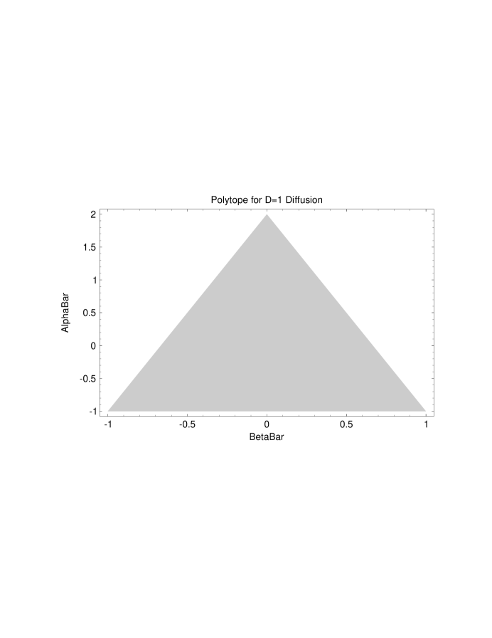
Figure 1: The Kinetic Polytope: Nonnegativity of the distribution function requires that the kinetic parameters ${\bar{\alpha}}$ and ${\bar{\beta}}$ lie in the shaded triangular region.

Note that the effect of varying $\rho$ at constant ${\bar{\alpha}}$ and ${\bar{\beta}}$ is to simply scale the components of the distribution function. The triangular region bounding the parameters ${\bar{\alpha}}$ and ${\bar{\beta}}$ is then independent of $\rho$. That is, the bounds on the barred kinetic parameters do not depend on the hydrodynamic parameter, so there is really no need for distinction between the master and kinetic polytopes. It should be noted that this is another nongeneric feature of the present model. While it is always possible to scale out by a single nonnegative-definite hydrodynamic parameter, as we have done with $\rho$ in this case, more sophisticated models will have several hydrodynamic parameters. In such cases, the shape of the region bounding the kinetic parameters will depend on the remaining hydrodynamic parameters. We shall see this more clearly in the example of Section 4.

3.3 Optimality of Representation

In this example, there is clearly a great deal of latitude in the choice of the kinetic bras. The only requirement that we have placed on these is that they be linearly independent of the hydrodynamic bra and of each other. This raises the question of whether there is some optimal choice that might be made for these. Of course, this depends entirely on what is meant by “optimal” in this context.

It has been noted that the original representation of $\left|{\bf N}\right\rangle$ is more natural for expressing the constraint of nonnegativity, while the conservation representation is more natural for expressing the collision process. For this reason, any computer implementation of entropic lattice Boltzmann methods will require frequent transformations between the two representations. This transformation is precisely what we have worked out in Eqs. (45) and (46) above. Thus, one natural figure of merit is the number of arithmetic operations required to perform such transformations.

To investigate this question, rather than requiring that the kinetic bras be given by Eqs. (40) and (42), we leave them in the general form

$$\left\langle{\mbox{\boldmath$\alpha$}}\right| = \left(\begin{array}[]{rrr}\alpha_{1}&\alpha_{2}&\alpha_{3}\end{array}\right)$$ (50)

$$\left\langle{\mbox{\boldmath$\beta$}}\right| = \left(\begin{array}[]{rrr}\beta_{1}&\beta_{2}&\beta_{3}\end{array}\right).$$ (52)

When we invert to get the kets, the results are

$$\begin{array}[]{ccccc}\left|{\mbox{\boldmath$\rho$}}\right\rangle=\frac{1}{\Delta}\left(\begin{array}[]{r}\alpha_{2}\beta_{3}-\alpha_{3}\beta_{2}\\ \alpha_{3}\beta_{1}-\alpha_{1}\beta_{3}\\ \alpha_{1}\beta_{2}-\alpha_{2}\beta_{1}\end{array}\right)&\phantom{aaa}&\left|{\mbox{\boldmath$\alpha$}}\right\rangle=\frac{1}{\Delta}\left(\begin{array}[]{r}\beta_{2}-\beta_{3}\\ \beta_{3}-\beta_{1}\\ \beta_{1}-\beta_{2}\end{array}\right)&\phantom{aaa}&\left|{\mbox{\boldmath$\beta$}}\right\rangle=\frac{1}{\Delta}\left(\begin{array}[]{r}\alpha_{3}-\alpha_{2}\\ \alpha_{1}-\alpha_{3}\\ \alpha_{2}-\alpha_{1}\end{array}\right),\end{array}$$ (53)

where we have defined the determinant

$$\Delta\equiv\alpha_{1}\left(\beta_{2}-\beta_{3}\right)+\alpha_{2}\left(\beta_{3}-\beta_{1}\right)+\alpha_{3}\left(\beta_{1}-\beta_{2}\right).$$ (54)

One way to simplify the transformation process would be to find a representation in which as many components as possible of the kinetic bras and kets vanish, without making the transformation singular. This means that we want to choose the $\alpha_{j}$’s and $\beta_{j}$’s such that $\Delta\neq 0$, while making vanish as many as possible of the following twelve quantities:

$$\alpha_{1}, \alpha_{2}, \alpha_{3},$$

$$\beta_{1}, \beta_{2}, \beta_{3},$$

$$\alpha_{3}-\alpha_{2}, \alpha_{1}-\alpha_{3}, \alpha_{2}-\alpha_{1},$$

$$\beta_{2}-\beta_{3}, \beta_{3}-\beta_{1}, \beta_{1}-\beta_{2}.$$

In this example, it is straightforward to see that there are a number of ways to make six of these quantities equal to zero. For example, we could choose

$$\alpha_{1}\neq 0, \alpha_{2}=0, \alpha_{3}=0,$$

$$\beta_{1}=0, \beta_{2}\neq 0, \beta_{3}=0,$$ (55)

resulting in $$\Delta=\alpha_{1}\beta_{2}\neq 0$$ and

$$\alpha_{3}-\alpha_{2}=0, \alpha_{1}-\alpha_{3}\neq 0, \alpha_{2}-\alpha_{1}\neq 0,$$

$$\beta_{2}-\beta_{3}\neq 0, \beta_{3}-\beta_{1}=0, \beta_{1}-\beta_{2}\neq 0.$$ (56)

This choice also has the added virtue of making the hydrodynamic ket equal to

$$\left|{\mbox{\boldmath$\rho$}}\right\rangle=\left(\begin{array}[]{c}0\\ 0\\ 1\end{array}\right),$$ (57)

which also has two vanishing components.

The computation of the $\left|{\bf N}\right\rangle$ components from the parameters $\rho$, ${\bar{\alpha}}$ and ${\bar{\beta}}$ is thus reduced to

$$N_{-} = \rho{\bar{\alpha}}$$

$$N_{0} = \rho{\bar{\beta}}$$

$$N_{+} = \rho\left(1-{\bar{\alpha}}-{\bar{\beta}}\right),$$

involving a total of two multiplications and two additions/subtractions; this may be contrasted with Eqs. (45) which involve six multiplications and five additions/subtractions. Likewise, using the choice of Eqs. (55), the computation of the parameters $\rho$, ${\bar{\alpha}}$ and ${\bar{\beta}}$ from the ${\bf N}$ is reduced to

$$\rho = N_{-}+N_{0}+N_{+}$$

$${\bar{\alpha}} = N_{-}/\rho$$

$${\bar{\beta}} = N_{0}/\rho,$$

involving two additions/subtractions and two divisions; this may be contrasted to Eqs. (46) which involve five additions/subtractions, one multiplication, and two divisions.

Clearly, more sophisticated figures of merit could be devised to optimize the transformations used in lattice Boltzmann computations. As we have noted, vanishing components of the kinetic bras and kets eliminate the addition/subtraction of terms. Likewise, components equal to $\pm 1$ do require an addition/subtraction, but not a multiplication, and this fact could be taken into account in a more refined figure of merit. The computation of the collision outcome is the principal “inner loop” of a lattice Boltzmann computation, insofar as it must be performed at each site of a spatial grid at each time step. Such considerations may be especially important for lattice Boltzmann models with large numbers of velocities.

3.4 Fourier-Motzkin Elimination

For this simple example, we had no difficulty visualizing the master and kinetic polytopes. In preparation for the succeeding sections where the task will be substantially more difficult, however, we take this opportunity to introduce the Fourier-Motzkin elimination method for this purpose. The algorithm consists of the following sequence of steps:

1. We rewrite the set of inequalities, Eq. (47) in matrix format,

   $$\left(\begin{array}[]{rrr}-\frac{\mbox{\scriptsize$1$}}{\mbox{\scriptsize$2$}}&+\frac{\mbox{\scriptsize$3$}}{\mbox{\scriptsize$2$}}&+1\\ +1&0&+1\\ -\frac{\mbox{\scriptsize$1$}}{\mbox{\scriptsize$2$}}&-\frac{\mbox{\scriptsize$3$}}{\mbox{\scriptsize$2$}}&+1\end{array}\right)\left(\begin{array}[]{c}{\bar{\alpha}}\\ {\bar{\beta}}\\ 1\end{array}\right)\geq 0$$ (58)

   We have adopted the convention of including constant terms in an extra column of the matrix, using the device of appending $1$ to the column vector of unknowns. In general, there will be $m$ inequalities for $n$ unknowns, and the matrix will be of size $m\times(n+1)$.

2. We scale each inequality by a positive factor so that the pivot  is either $-1$, $0$ or $+1$. (Recall that scaling by a positive factor preserves the sense of an inequality.) We then reorder the inequalities, sorting by their (scaled) pivots so that the zero pivots are last. Beginning with Eq. (58), this yields

   $$\left(\begin{array}[]{rrr}-1&+3&+2\\ -1&-3&+2\\ +1&0&+1\end{array}\right)\left(\begin{array}[]{c}{\bar{\alpha}}\\ {\bar{\beta}}\\ 1\end{array}\right)\geq 0.$$ (59)

   Note that there were no zero pivots in this first step. We did, however, reorder the inequalities so that those with pivot $-1$ are together, and preceed that with pivot $+1$.

3. We now add all pairs of inequalities, such that the first member of the pair has pivot $-1$ and the second member of the pair has pivot $+1$, and we append the new zero-pivot inequalities thus obtained to the system. If there are $m_{-}$ inequalities with pivot $-1$, and $m_{+}$ inequalities with pivot $+1$, this results in the addition of $m_{-}m_{+}$ new inequalities to the system. Since there were $m-m_{-}-m_{+}$ zero-pivot inequalities to begin with, the new system will have a total of $m_{0}=m-m_{-}-m_{+}+m_{-}m_{+}$ zero-pivot inequalities. For our above example, $m=3$, $m_{-}=2$ and $m_{+}=1$, so we get $m_{0}=2$ zero-pivot inequalities in the system, which can now be written

   $$\left(\begin{array}[]{rrr}-1&+3&+2\\ -1&-3&+2\\ +1&0&+1\\ 0&+3&+3\\ 0&-3&+3\\ \end{array}\right)\left(\begin{array}[]{c}{\bar{\alpha}}\\ {\bar{\beta}}\\ 1\end{array}\right)\geq 0.$$ (60)

4. Finally, we recurse by returning to step 2 for the $m_{0}\times n$ submatrix obtained by taking only the zero-pivot inequalities and neglecting the first unknown (since the zero-pivot inequalities do not involve it anyway). We continue in this fashion until all of the first $n$ elements of the rows of the matrix are zero.

For our example, the recursion step asks us to return to step 2 for the submatrix indicated below

$$\left(\mbox{ \begin{tabular}[]{r|rr}\lx@intercol\hfil-1\lx@intercol &\lx@intercol\hfil+3\lx@intercol &\lx@intercol\hfil+2\lx@intercol\\ \lx@intercol\hfil-1\lx@intercol &\lx@intercol\hfil-3\lx@intercol &\lx@intercol\hfil+2\lx@intercol\\ \lx@intercol\hfil+1\lx@intercol &\lx@intercol\hfil 0\lx@intercol &\lx@intercol\hfil+1\lx@intercol\\ \cline{2-3}\cr\\ 0&+3&+3\\ 0&-3&+3\end{tabular} }\right)\left(\begin{array}[]{c}{\bar{\alpha}}\\ {\bar{\beta}}\\ 1\end{array}\right)\geq 0.$$ (61)

As before, we begin by normalizing the rows and sorting them by pivot,

$$\left(\mbox{ \begin{tabular}[]{r|rr}\lx@intercol\hfil-1\lx@intercol &\lx@intercol\hfil+3\lx@intercol &\lx@intercol\hfil+2\lx@intercol\\ \lx@intercol\hfil-1\lx@intercol &\lx@intercol\hfil-3\lx@intercol &\lx@intercol\hfil+2\lx@intercol\\ \lx@intercol\hfil+1\lx@intercol &\lx@intercol\hfil 0\lx@intercol &\lx@intercol\hfil+1\lx@intercol\\ \cline{2-3}\cr\\ 0&-1&+1\\ 0&+1&+1\end{tabular} }\right)\left(\begin{array}[]{c}{\bar{\alpha}}\\ {\bar{\beta}}\\ 1\end{array}\right)\geq 0.$$ (62)

In this example there is now one row of the submatrix with pivot $-1$ and one with pivot $+1$, so we append the sum of these to the system to get

$$\left(\mbox{ \begin{tabular}[]{r|rr}\lx@intercol\hfil-1\lx@intercol &\lx@intercol\hfil+3\lx@intercol &\lx@intercol\hfil+2\lx@intercol\\ \lx@intercol\hfil-1\lx@intercol &\lx@intercol\hfil-3\lx@intercol &\lx@intercol\hfil+2\lx@intercol\\ \lx@intercol\hfil+1\lx@intercol &\lx@intercol\hfil 0\lx@intercol &\lx@intercol\hfil+1\lx@intercol\\ \cline{2-3}\cr\\ 0&-1&+1\\ 0&+1&+1\\ 0&0&+2\end{tabular} }\right)\left(\begin{array}[]{c}{\bar{\alpha}}\\ {\bar{\beta}}\\ 1\end{array}\right)\geq 0.$$ (63)

At this point, the first $n$ elements of the last row of the matrix are zero, so we stop the recursion and examine the last row. It states a true inequality, namely $+2\geq 0$, so we can conclude that the original inequalities are not mutually exclusive; that is, a nonnull polytope of solutions will exist. If the $n+1$ element of the final row had been negative, we would have concluded that no such solution was possible.

Once we have stopped the recursion and established the consistency of the inequalities, we can get the final set of inequalities by “back substituting” up the matrix. The last two nontrivial inequalities tell us that $-1\leq{\bar{\beta}}\leq+1$, or

$$\left|{\bar{\beta}}\right|\leq 1.$$ (64)

The first three equations then yield $-1\leq{\bar{\alpha}}\leq\min\left(2-3{\bar{\beta}},2+3{\bar{\beta}}\right)$ which is equivalent to Eq. (48), describing the triangular region of Fig. 1.

More generally, each variable will have a lower bound that is the maximum of all the lower bounds determined by the inequalities with pivot $+1$, and an upper bound that is the minimum of all the upper bounds determined by the inequalities with pivot $-1$. The arguments of the maximum and minimum functions will depend only on those variables that have already been bounded. If we were using the technique to find limits of integration for a multiple integral, the inequalities at the bottom of the Fourier-Motzkin-eliminated matrix would correspond to the outermost integrals. We shall revisit this technique in the next section.

3.5 Collision Operator

To illustrate the construction of an entropically stable collision operator for this model, we adopt the simplest possible $H$ function by taking $\zeta_{j}(x)=x$. Since there is only one hydrodynamic degree of freedom, Eqs. (27) reduce to

$${N^{\mbox{\scriptsize eq}}_{-}}={N^{\mbox{\scriptsize eq}}_{0}}={N^{\mbox{\scriptsize eq}}_{+}}=\frac{1}{Q}.$$ (65)

Eq. (28) then tells us that $Q=3/\rho$, so

$${{\bf N}^{\mbox{\scriptsize eq}}}=\frac{\rho}{3}\left(\begin{array}[]{c}1\\ 1\\ 1\end{array}\right).$$ (66)

Comparing this with Eq. (45), we see that, within the kinetic polytope, the equilibrium point is the origin, $\alpha^{\mbox{\scriptsize eq}}=\beta^{\mbox{\scriptsize eq}}=0$. A contour plot of the $H$ function on the kinetic polytope is presented in Fig. 2.

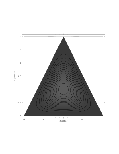
Figure 2: $H$ Function on the Kinetic Polytope: Note that $H$ reaches a maximum when ${\bar{\alpha}}={\bar{\beta}}=0$, and goes to $-\infty$ on the boundary of the polytope.

The lattice BGK equation in the conservation representation, Eq. (30), is then equivalent to the prescription

$$\rho^{\prime}=\rho$$ (67)

and

$$\left(\begin{array}[]{l}\alpha^{\prime}\\ \beta^{\prime}\end{array}\right)=\left(\begin{array}[]{l}\alpha\\ \beta\end{array}\right)+\frac{1}{\tau}\left[\left(\begin{array}[]{l}\alpha^{\mbox{\scriptsize eq}}\\ \beta^{\mbox{\scriptsize eq}}\end{array}\right)-\left(\begin{array}[]{l}\alpha\\ \beta\end{array}\right)\right]=z\left(\begin{array}[]{l}\alpha\\ \beta\end{array}\right),$$ (68)

where $z\equiv 1-1/\tau$. These can also be written as the single equation

$$\left(\begin{array}[]{l}\rho^{\prime}\\ \alpha^{\prime}\\ \beta^{\prime}\end{array}\right)=\left(\begin{array}[]{ccc}1&0&0\\ 0&z&0\\ 0&0&z\end{array}\right)\left(\begin{array}[]{l}\rho\\ \alpha\\ \beta\end{array}\right).$$ (69)

As promised, the collision is dramatically simplified in this representation. The hydrodynamic parameter is unchanged; only the two kinetic parameters are altered by the collision. Transformation back to the original representation yields

$$\left|{\bf N}^{\prime}\right\rangle=\frac{\rho}{3}\left(\begin{array}[]{c}1-\frac{z{\bar{\alpha}}}{2}+\frac{3z{\bar{\beta}}}{2}\\ 1+z{\bar{\alpha}}\\ 1-\frac{z{\bar{\alpha}}}{2}-\frac{3z{\bar{\beta}}}{2}\\ \end{array}\right),$$ (70)

or equivalently

$$\left|{\bf N}^{\prime}\right\rangle=\frac{1}{3}\left(\begin{array}[]{ccc}1+2z&1-z&1-z\\ 1-z&1+2z&1-z\\ 1-z&1-z&1+2z\end{array}\right)\left|{\bf N}\right\rangle.$$ (71)

3.6 Entropic Stabilization

The condition for marginal entropic stabilization, Eq. (31), for this model is then

$$\ln N^{\prime}_{+}+\ln N^{\prime}_{0}+\ln N^{\prime}_{-}=\ln N_{+}+\ln N_{0}+\ln N_{-}.$$ (72)

This needs to be solved for the limiting value $z=z_{*}$, where $z_{*}=1-1/\tau_{*}$. Using Eqs. (45) and (70), this becomes

$$\left(1-\frac{z_{*}{\bar{\alpha}}}{2}+\frac{3z_{*}{\bar{\beta}}}{2}\right)\left(1+z_{*}{\bar{\alpha}}\right)\left(1-\frac{z_{*}{\bar{\alpha}}}{2}-\frac{3z_{*}{\bar{\beta}}}{2}\right)=\left(1-\frac{{\bar{\alpha}}}{2}+\frac{3{\bar{\beta}}}{2}\right)\left(1+{\bar{\alpha}}\right)\left(1-\frac{{\bar{\alpha}}}{2}-\frac{3{\bar{\beta}}}{2}\right).$$ (73)

This appears to be a cubic equation for $z_{*}$, but in fact $z_{*}=1$ (corresponding to $\tau_{*}\rightarrow\infty$) is clearly a root. It is an uninteresting root since it corresponds to no collision. Once it is removed, we are left with a quadratic for $z_{*}$, so the relevant solution is easily written in closed form,

$$z_{*}=\frac{3{\bar{\alpha}}^{2}-{\bar{\alpha}}^{3}+9{\bar{\beta}}^{2}+9{\bar{\alpha}}{\bar{\beta}}^{2}-\sqrt{3({\bar{\alpha}}^{2}+{\bar{\alpha}}^{3}+3{\bar{\beta}}^{2}-9{\bar{\alpha}}{\bar{\beta}}^{2})(3{\bar{\alpha}}^{2}-{\bar{\alpha}}^{3}+9{\bar{\beta}}^{2}+9{\bar{\alpha}}{\bar{\beta}}^{2})}}{2({\bar{\alpha}}^{3}-9{\bar{\alpha}}{\bar{\beta}}^{2})}.$$ (74)

A contour plot of the function $z_{*}({\bar{\alpha}},{\bar{\beta}})$ on the kinetic polytope is displayed in Fig. 3. There it can be seen that $z_{*}$ has minimum value of $-2$ at the midpoints of the sides of the triangle, has maximum value of $-1/2$ at the vertices, and approaches $-1$ at the equilibrium ${\bar{\alpha}}={\bar{\beta}}=0$.

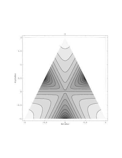
Figure 3: Contours of $z_{*}({\bar{\alpha}},{\bar{\beta}})$ on the Kinetic Polytope: This function approaches $-1$ when ${\bar{\alpha}}={\bar{\beta}}=0$, is $-2$ on the midpoints of the sides of the triangle, and is $-1/2$ at the vertices.

The entropically stabilized collision operator is then given by Eq. (70), with $\tau\rightarrow\tau_{*}/\kappa$, or equivalently

$$z\rightarrow 1-\kappa(1-z_{*}).$$ (75)

It is useful to discuss three possible choices for $\kappa$:

• $\kappa\rightarrow 0$ means that $z\rightarrow 1$ and $\tau\rightarrow\infty$. This is the uninteresting limit in which the collision operator vanishes and hydrodynamic behavior is lost.

• $\kappa=1/2$ means that $z=(1+z_{*})/2$ and $\tau=2/(1-z_{*})$. This is interesting because near equilibrium, where $z_{*}\sim-1$, it coincides with the prescription $\tau=1$. This is the limit, mentioned in Subsection 2.9, wherein the outgoing state is the local equilibrium. This is the smallest value of $\tau$ for which the standard lattice BGK algorithm is guaranteed to be stable. (In fairness, the standard algorithm is likely to be stable for smaller $\tau$; it’s just that this is not guaranteed.)

• $\kappa\rightarrow 1$ means that $z\rightarrow z_{*}$ and $\tau\rightarrow\tau_{*}$. This is the largest value of $\tau$ for which the entropic lattice BGK algorithm is guaranteed to be stable.

3.7 Attainable Transport Coefficient

The complicated form of Eq. (74) may lead one to believe that the hydrodynamic equation (in this case, a diffusion equation) would be very difficult to derive for the entropically stabilized collision operator. In fact, this is not the case at all. The Chapman-Enskog analysis that yields the hydrodynamic equations requires only that one linearize the collision operator about the local equilibrium. Since the local equilibrium has $\alpha=\beta=0$, it is clear from Eqs. (68) and (69), that only the value of $z$ at equilibrium will enter. Since $z_{*}\rightarrow-1$ at the equilibrium, Eq. (75) indicates that the transport coefficient will be precisely that obtained by the standard lattice BGK algorithm with $\tau=1/(2\kappa)$.

The Chapman-Enskog analysis of the standard lattice BGK algorithm is an elementary exercise [28]. The result for the diffusivity in natural lattice units is

$$D=\frac{1}{3}\left(\tau-\frac{1}{2}\right).$$ (76)

Hence, by the above argument, the result for the diffusivity of the entropic lattice BGK algorithm is

$$D=\frac{1}{6}\left(\frac{1}{\kappa}-1\right).$$ (77)

From this, we can clearly see the benefit of the entropic algorithm. The standard lattice BGK algorithm is not guaranteed stable for $\tau<1$ or $\kappa>1/2$, as discussed above. From Eq. (76) or (77), respectively, we see that this corresponds to a minimum diffusivity of $1/6$. By contrast, the entropic lattice BGK algorithm loses stability only when $\kappa=1$, corresponding to $D=0$.

It is remarkable that we have found a stable, conservative, explicit algorithm that seems to allow the transport coefficient to become arbitrarily small. After all, the analysis leading to the shear viscosity of a fluid model is not very different from that leading to the diffusivity above, and arbitrarily small shear viscosity would allow for arbitrarily large Reynolds number. In the field of computational fluid dynamics, however, results that seem too good to be true usually are just that. For one thing, stability does not imply accuracy. A perfectly stable algorithm is not terribly useful if it does not converge to the correct answer. Flows at higher Reynolds number involve ever smaller eddies, and at some point the lattice spacing becomes insufficient to resolve these. While it is comforting to have an algorithm that does not lose stability in this situation, it is probably a mistake to attach much physical significance to its results.

Another problem is that the time required for the system to come to equilibrium goes to infinity as $\kappa\rightarrow 1$. In fact, when $\kappa=1$ the entropic lattice BGK collision operator is its own inverse: If incoming state $\left|{\bf N}\right\rangle$ yields outgoing state $\left|{\bf N}^{\prime}\right\rangle$, then incoming state $\left|{\bf N}^{\prime}\right\rangle$ would yield outgoing state $\left|{\bf N}\right\rangle$. This means that if the entire lattice were initialized slightly away from equilibrium with no spatial gradients whatsoever, it would simply thrash back and forth between two states, without ever converging to the desired equilibrium. When the time required to achieve local equilibrium exceeds time scales of interest, hydrodynamic behavior breaks down.

To illustrate this problem, we simulated the entropically stabilized diffusion model with the initial density profile

$$\rho=\rho_{0}+\rho_{1}\sin\left(\frac{2\pi\ell x}{L}\right)$$ (78)

on a periodic lattice. We used lattice size $L=32$, and wavenumber $\ell=3$ in all the simulations reported below. We initialized the state of each site in a local equilibrium $N_{-}=N_{0}=N_{+}=\rho/3$, without the Chapman-Enskog correction due to gradient. Now Eq. (78) is a solution of the diffusion equation, if $\rho_{1}$ decays in time as $\exp(-\gamma t)$, where

$$\gamma=D\left(\frac{2\pi\ell}{L}\right)^{2}.$$ (79)

So we fit our results to the functional form of Eq. (78), measured $\rho_{1}(t)$, and did a least-squares fit of its logarithm to a linear function of time in order to determine $\gamma$. We then used Eq. (79) to get the diffusion coefficient, and we compared this to the theoretical value provided by Eq. (77) for several different values of $\kappa$, approaching unity.

Fig. 4 shows the measured value of $\rho_{1}(t)$ for $\kappa=0.9$ and $\kappa=0.99$.

Figure 4: Decay of sinusoidal density profile for $\kappa=0.9$ (left) and $\kappa=0.99$ (right).

As can be seen, there is an initial transient, due to the inadequacy of the form used for the local equilibrium $N_{-}=N_{0}=N_{+}=\rho/3$ in the presence of a spatial gradient. The left-hand side of Fig. 5 shows the measured value of $\rho_{1}(t)$ for $\kappa=0.999$, and the right-hand side is an enlargement of the transient region. Fig. 6 shows the same things for $\kappa=0.9999$. Note that the transient period lengthens considerably as $\kappa$ nears unity. We could have substantially reduced these transient periods had we used the Chapman-Enskog correction to the local equilibrium; instead, we simply waited for the transient to die away before measuring the decay constant $\gamma$.

Figure 5: Decay of sinusoidal density profile for $\kappa=0.999$

Figure 6: Decay of sinusoidal density profile for $\kappa=0.9999$

The results for the diffusivity are displayed in Table 1. Note that we find reasonable agreement until we get to the cases $\kappa=0.9999$ and $\kappa=0.99999$. To see what is going wrong for these cases, the upper-left-hand corner of Fig. 7 shows the measured value of $\rho_{1}(t)$ for $\kappa=0.99999$, and the upper-right-hand corner shows the same plot with a reduced range for the ordinate. In addition to the oddly shaped envelope of the initial transient period, similar to that seen in Fig. 6, and enlarged in the lower part of this figure, we note that the plot of $\rho_{1}(t)$ in the upper right seems to be increasing in thickness, even after the initial transient. Upon further enlargement, shown on the left-hand side of Fig. 8, we see that this thickness is in fact a subtle transient of extremely long duration. The right-hand side of the figure shows this same transient at the longest time for which the simulation in Fig. 7 was run. Though reduced in magnitude (the scales of the ordinates of both graphs in Fig. 8 are equal), the transient is still present, even though most of the signal itself has diffused away. We believe that this transient is causing the anomaly in the measured diffusivity. A much longer simulation would be required to test this assertion.

$\kappa$	$D_{\mbox{\scriptsize theory}}$	$D_{\mbox{\scriptsize meas}}$
$0.9$	$1.852\times 10^{-2}$	$1.75364\times 10^{-2}$
$0.99$	$1.684\times 10^{-3}$	$1.67419\times 10^{-3}$
$0.999$	$1.668\times 10^{-4}$	$1.66674\times 10^{-4}$
$0.9999$	$1.667\times 10^{-5}$	$1.66198\times 10^{-5}$
$0.99999$	$1.667\times 10^{-6}$	$2.28751\times 10^{-6}$

Table 1: Theoretical and measured values of the diffusivity for various values of $\kappa$.

Figure 7: Decay of sinusoidal density profile for $\kappa=0.99999$

Figure 8: Decay of sinusoidal density profile for $\kappa=0.99999$

To better understand this loss of separation between the kinetic and hydrodynamic time scales, note that the time required for the signal to decay away is

$$\tau_{\mbox{\scriptsize signal}}\propto\frac{1}{\gamma}\propto\frac{1}{D}\propto\frac{\kappa}{1-\kappa}.$$ (80)

The time required for the transient to decay to $1/e$ of its initial value, on the other hand, obeys

$$\kappa^{\tau_{\mbox{\scriptsize transient}}}=\frac{1}{e},$$ (81)

whence

$$\tau_{\mbox{\scriptsize transient}}\propto\frac{1}{\ln\kappa}.$$ (82)

For $\kappa=1-\epsilon$, where $\epsilon$ is small, the characteristic times in Eqs. (80) and (82) both go like $1/\epsilon$. Thus, the transients begin to linger for hydrodynamic time scales, and it becomes impossible to separate the kinetic behavior from the hydrodynamic behavior.

When the time required for the decay of transients is comparable to hydrodynamic time scales of interest, the usefulness of the simulation is questionable. Thus, while Table 1 indicates good agreement with theory, and the transport coefficient really does tend to zero without loss of stability, one must be exceedingly careful in the preparation of the initial condition to exploit this feature of entropic lattice Boltzmann models. In particular, transient behavior could be dramatically reduced by including the Chapman-Enskog correction to first-order in the gradient. Indeed, if this problem turns out to be the only obstacle to stable, conservative, explicit algorithms with arbitrarily small transport coefficients, higher-order gradient corrections may also be worth investigating.

4 One-Dimensional Compressible Fluid Model

In this section, we apply the entropic lattice Boltzmann method to a simple five-velocity model of fluid dynamics in one dimension, first considered by Renda et al. in 1997 [14]. We shall find that the geometric picture is much richer than that for the diffusion model. The master polytope for this model is four-dimensional, and we shall show that the Fourier-Motzkin algorithm is very useful for describing it.

4.1 Description of Model

As a second example, we consider a lattice Boltzmann model for a one-dimensional compressible fluid with conserved mass, momentum and energy, first studied by Renda et al. [14]. The velocity space of this model consists of five discrete values of velocity, namely $0$, $\pm 1$, and $\pm 2$. The single-particle distribution at site $x$ with velocity $j\in\{-2,-1,0,+1,+2\}$ is denoted by $N_{j}$. As in the last example, the state vector $\left|{\bf N}\right\rangle$ at a given site $x$ will be denoted by a ket,

$$\left|{\bf N}\right\rangle=\left(\begin{array}[]{l}N_{-2}\\ N_{-1}\\ N_{0}\\ N_{+1}\\ N_{+2}\end{array}\right),$$ (83)

where we have suppressed the dependence on $x$ for simplicity.

A compressible fluid conserves mass, momentum and kinetic energy, so we suppose that the corresponding densities

$$\rho = \sum_{j=-2}^{+2}N_{j}=\left\langle{\mbox{\boldmath$\rho$}}\mid{\bf N}\right\rangle$$ (84)

$$\pi = \sum_{j=-2}^{+2}j\;N_{j}=\left\langle{\mbox{\boldmath$\pi$}}\mid{\bf N}\right\rangle$$ (85)

$$\varepsilon = \sum_{j=-2}^{+2}\frac{j^{2}}{2}\;N_{j}=\left\langle{\mbox{\boldmath$\varepsilon$}}\mid{\bf N}\right\rangle,$$ (86)

are conserved by the collisions. Here we have introduced the bras

$$\begin{array}[]{ccc}\left\langle{\mbox{\boldmath$\rho$}}\right|_{j}&=&1\\ &&\\ \left\langle{\mbox{\boldmath$\pi$}}\right|_{j}&=&j\\ &&\\ \left\langle{\mbox{\boldmath$\varepsilon$}}\right|_{j}&=&j^{2}/2,\end{array}$$ (92)

or explicitly

$$\left\langle{\mbox{\boldmath$\rho$}}\right| \equiv \phantom{\frac{1}{2}}\left(\begin{array}[]{rrrrr}+1&+1&+1&+1&+1\end{array}\right)$$ (94)

$$\left\langle{\mbox{\boldmath$\pi$}}\right| \equiv \phantom{\frac{1}{2}}\left(\begin{array}[]{rrrrr}-2&-1&\phantom{+}0&+1&+2\end{array}\right)$$ (96)

$$\left\langle{\mbox{\boldmath$\varepsilon$}}\right| \equiv \frac{\mbox{\scriptsize$1$}}{\mbox{\scriptsize$2$}}\left(\begin{array}[]{rrrrr}+4&+1&\phantom{+}0&+1&+4\end{array}\right).$$ (98)

These are the three hydrodynamic degrees of freedom in this example. Because there are a total of five degrees of freedom, the other two must be kinetic in nature. To span these kinetic degrees of freedom and thereby make the bra basis complete, we introduce the linearly independent bras,

$$\left\langle{\mbox{\boldmath$\alpha$}}\right| = \frac{\mbox{\scriptsize$1$}}{\mbox{\scriptsize$2$}}\left(\begin{array}[]{rrrrr}\phantom{-}0&+1&\phantom{-}0&+1&\phantom{-}0\end{array}\right)$$ (100)

$$\left\langle{\mbox{\boldmath$\beta$}}\right| = \frac{\mbox{\scriptsize$1$}}{\mbox{\scriptsize$2$}}\left(\begin{array}[]{rrrrr}\phantom{-}0&-1&\phantom{-}0&+1&\phantom{-}0\end{array}\right).$$ (102)

Next, we form a matrix of the five bras and invert it to get the dual basis of kets,

$$\left(\begin{array}[]{ccccc}\left|{\mbox{\boldmath$\rho$}}\right\rangle&\left|{\mbox{\boldmath$\pi$}}\right\rangle&\left|{\mbox{\boldmath$\varepsilon$}}\right\rangle&\left|{\mbox{\boldmath$\alpha$}}\right\rangle&\left|{\mbox{\boldmath$\beta$}}\right\rangle\end{array}\right)=$$ (120)

$$\left(\begin{array}[]{c}\left\langle{\mbox{\boldmath$\rho$}}\right|\\ \left\langle{\mbox{\boldmath$\pi$}}\right|\\ \left\langle{\mbox{\boldmath$\varepsilon$}}\right|\\ \left\langle{\mbox{\boldmath$\alpha$}}\right|\\ \left\langle{\mbox{\boldmath$\beta$}}\right|\end{array}\right)^{-1}=\left[\frac{1}{2}\left(\begin{array}[]{rrrrr}+2&+2&+2&+2&+2\\ -4&-2&0&+2&+4\\ +4&+1&0&+1&+4\\ 0&+1&0&+1&0\\ 0&-1&0&+1&0\end{array}\right)\right]^{-1}=\frac{1}{4}\left(\begin{array}[]{rrrrr}0&-1&+1&-1&+2\\ 0&0&0&+4&-4\\ +4&0&-2&-6&0\\ 0&0&0&+4&+4\\ 0&+1&+1&-1&-2\end{array}\right).$$

From Eq. (120) we identify the linearly independent basis kets, consisting of the hydrodynamic basis kets

$$\begin{array}[]{lll}\left|{\mbox{\boldmath$\rho$}}\right\rangle=\phantom{\frac{1}{4}}\left(\begin{array}[]{r}0\\ 0\\ +1\\ 0\\ 0\end{array}\right),&\left|{\mbox{\boldmath$\pi$}}\right\rangle=\frac{1}{4}\left(\begin{array}[]{r}-1\\ 0\\ 0\\ 0\\ +1\end{array}\right),&\left|{\mbox{\boldmath$\varepsilon$}}\right\rangle=\frac{1}{4}\left(\begin{array}[]{r}+1\\ 0\\ -2\\ 0\\ +1\end{array}\right),\end{array}$$ (121)

and the kinetic basis kets

$$\begin{array}[]{ll}\left|{\mbox{\boldmath$\alpha$}}\right\rangle=\frac{1}{4}\left(\begin{array}[]{r}-1\\ +4\\ -6\\ +4\\ -1\end{array}\right),&\left|{\mbox{\boldmath$\beta$}}\right\rangle=\frac{1}{2}\left(\begin{array}[]{r}+1\\ -2\\ 0\\ +2\\ -1\end{array}\right).\end{array}$$ (122)

Unlike the previous example, there is no obvious correspondence between the individual bra and ket basis elements. This is because there is no natural notion of a metric in this space. Nevertheless, as noted in Section 2, it is always possible to construct an entire ket basis from an entire bra basis, and that is what we have done here.

We can then expand the state ket in this basis as follows

$$\left|{\bf N}\right\rangle=\rho\left|{\mbox{\boldmath$\rho$}}\right\rangle+\pi\left|{\mbox{\boldmath$\pi$}}\right\rangle+\varepsilon\left|{\mbox{\boldmath$\varepsilon$}}\right\rangle+\alpha\left|{\mbox{\boldmath$\alpha$}}\right\rangle+\beta\left|{\mbox{\boldmath$\beta$}}\right\rangle=\rho\left(\begin{array}[]{c}\frac{\mbox{\scriptsize$1$}}{\mbox{\scriptsize$4$}}\left({\bar{\varepsilon}}-{\bar{\pi}}-{\bar{\alpha}}+2{\bar{\beta}}\right)\\ {\bar{\alpha}}-{\bar{\beta}}\\ 1-\frac{\mbox{\scriptsize$1$}}{\mbox{\scriptsize$2$}}\left({\bar{\varepsilon}}+3{\bar{\alpha}}\right)\\ {\bar{\alpha}}+{\bar{\beta}}\\ \frac{\mbox{\scriptsize$1$}}{\mbox{\scriptsize$4$}}\left({\bar{\varepsilon}}+{\bar{\pi}}-{\bar{\alpha}}-2{\bar{\beta}}\right)\end{array}\right),$$ (123)

where we have continued to use an overbar to denote conserved quantities per unit mass; for example, ${\bar{\pi}}\equiv\pi/\rho$ is the hydrodynamic velocity. As with the last example, this representation of the distribution function $\left|{\bf N}\right\rangle$ has the virtue of making the conserved quantities manifest. In this case, we have the inverse transformation

$$\rho = \left\langle{\mbox{\boldmath$\rho$}}\mid{\bf N}\right\rangle=+N_{-2}+N_{-1}+N_{0}+N_{+1}+N_{+2}$$

$$\pi = \left\langle{\mbox{\boldmath$\pi$}}\mid{\bf N}\right\rangle=-2N_{-2}-N_{-1}+N_{+1}+2N_{+2}$$

$$\varepsilon = \left\langle{\mbox{\boldmath$\varepsilon$}}\mid{\bf N}\right\rangle=+2N_{-2}+N_{-1}/2+N_{+1}/2+2N_{+2}$$ (124)

$$\alpha = \left\langle{\mbox{\boldmath$\alpha$}}\mid{\bf N}\right\rangle=+N_{-1}/2+N_{+1}/2$$

$$\beta = \left\langle{\mbox{\boldmath$\beta$}}\mid{\bf N}\right\rangle=-N_{-1}/2+N_{+1}/2.$$

4.2 Nonnegativity

We now consider the shape of the master and kinetic polytopes for the compressible fluid model described in the last subsection. Here we shall find a much richer structure than the simple triangular region that we found for the diffusive example in the last section above. Referring to Eq. (123), we see that that nonnegativity of the components of the single-particle distribution function is guaranteed by the set of inequalities $\rho\geq 0$ and

$$0 \leq {\bar{\varepsilon}}-{\bar{\pi}}-{\bar{\alpha}}+2{\bar{\beta}}$$

$$0 \leq {\bar{\alpha}}-{\bar{\beta}}$$

$$0 \leq 2-{\bar{\varepsilon}}-3{\bar{\alpha}}$$ (125)

$$0 \leq {\bar{\alpha}}+{\bar{\beta}}$$

$$0 \leq {\bar{\varepsilon}}+{\bar{\pi}}-{\bar{\alpha}}-2{\bar{\beta}}.$$

These define the master polytope in the four dimensional $({\bar{\pi}},{\bar{\varepsilon}},{\bar{\alpha}},{\bar{\beta}})$ space. If we fix the hydrodynamic parameters, ${\bar{\pi}}$ and ${\bar{\varepsilon}}$, the above still constitute a set of linear inequalities specifying the corresponding kinetic polytope in the two dimensional $({\bar{\alpha}},{\bar{\beta}})$ space. Geometrically, these are the intersections of the master polytope with the (hyper)planes of fixed hydrodynamic parameters ${\bar{\pi}}$ and ${\bar{\varepsilon}}$. Thus, though the mass density $\rho$ still scales out of the distribution function, the shape of the kinetic polytopes in the $({\bar{\alpha}},{\bar{\beta}})$ plane will depend on the hydrodynamic velocity ${\bar{\pi}}$ and the kinetic energy per unit mass ${\bar{\varepsilon}}$.

It is not particularly easy to visualize the shape of the kinetic polytope in the $({\bar{\alpha}},{\bar{\beta}})$ plane for given hydrodynamic parameters ${\bar{\pi}}$ and ${\bar{\varepsilon}}$. In fact, the task is tedious enough that we have relegated it to Appendix A, which takes the reader on a detailed tour of the four-dimensional master polytope and its kinetic polytope cross sections. To summarize the conclusions of that Appendix, the projection of the master polytope on the $({\bar{\pi}},{\bar{\varepsilon}})$ plane is illustrated in Fig. 9. Values of $({\bar{\pi}},{\bar{\varepsilon}})$ outside the shaded regions are not possible. The shape of the kinetic polytope is then a triangle when $({\bar{\pi}},{\bar{\varepsilon}})$ is in the most lightly shaded regions of Fig. 9, a quadrilateral when $({\bar{\pi}},{\bar{\varepsilon}})$ is in the intermediately shaded regions of Fig. 9, and a pentagon when $({\bar{\pi}},{\bar{\varepsilon}})$ is in the most darkly shaded region of Fig. 9. Illustrations and detailed descriptions of the kinetic polytopes for particular values of $({\bar{\pi}},{\bar{\varepsilon}})$ in each of the seven distinct regions with ${\bar{\pi}}\geq 0$ are provided in the seven figures of Appendix A; the chart below Fig. 9 indicates which figure corresponds to each of its regions. Finally, since the inequalities are invariant under $({\bar{\pi}},{\bar{\beta}})\rightarrow(-{\bar{\pi}},-{\bar{\beta}})$, the kinetic polytopes for ${\bar{\pi}}\leq 0$ are obtained from those for ${\bar{\pi}}\geq 0$ by simply reflecting in ${\bar{\beta}}$.

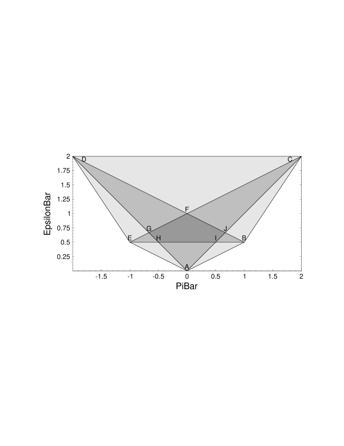
Figure 9: Bounds on ${\bar{\pi}}$ and ${\bar{\varepsilon}}$: The regions with the lightest shading correspond to triangular regions in the $({\bar{\alpha}},{\bar{\beta}})$ plane, those with intermediate shading correspond to quadrilateral regions in the $({\bar{\alpha}},{\bar{\beta}})$ plane, and that with the darkest shading corresponds to pentagonal regions in the $({\bar{\alpha}},{\bar{\beta}})$ plane.

4.3 Fourier-Motzkin Analysis for the 1D Compressible Fluid Model

To compute the master polytope for the compressible fluid model, we cast the inequalities of Eqs. (125) into matrix format as follows,

$$\left(\begin{array}[]{rrrrr}-1&+2&-1&+1&0\\ +1&-1&0&0&0\\ -3&0&0&-1&+2\\ +1&+1&0&0&0\\ -1&-2&+1&+1&0\end{array}\right)\left(\begin{array}[]{c}{\bar{\alpha}}\\ {\bar{\beta}}\\ {\bar{\pi}}\\ {\bar{\varepsilon}}\\ 1\end{array}\right)\geq 0.$$ (126)

Here we have put the hydrodynamic parameters ${\bar{\pi}}$ and ${\bar{\varepsilon}}$ after the kinetic parameters ${\bar{\alpha}}$ and ${\bar{\beta}}$ in the column vector of unknowns, for reasons that will become apparent in a moment. Performing the Fourier-Motzkin algorithm on this set of inequalities, we finally arrive at the 23 inequalities,

$$\left(\begin{array}[]{rrrrr}-1&-2&+1&+1&0\\ -1&+2&-1&+1&0\\ -1&0&0&-\frac{\mbox{\scriptsize$1$}}{\mbox{\scriptsize$3$}}&+\frac{\mbox{\scriptsize$2$}}{\mbox{\scriptsize$3$}}\\ +1&-1&0&0&0\\ +1&+1&0&0&0\\ 0&-1&+1&+1&0\\ 0&-1&+\frac{\mbox{\scriptsize$1$}}{\mbox{\scriptsize$3$}}&+\frac{\mbox{\scriptsize$1$}}{\mbox{\scriptsize$3$}}&0\\ 0&-1&0&-\frac{\mbox{\scriptsize$1$}}{\mbox{\scriptsize$3$}}&+\frac{\mbox{\scriptsize$2$}}{\mbox{\scriptsize$3$}}\\ 0&+1&-1&+1&0\\ 0&+1&-\frac{\mbox{\scriptsize$1$}}{\mbox{\scriptsize$3$}}&+\frac{\mbox{\scriptsize$1$}}{\mbox{\scriptsize$3$}}&0\\ 0&+1&0&-\frac{\mbox{\scriptsize$1$}}{\mbox{\scriptsize$3$}}&+\frac{\mbox{\scriptsize$2$}}{\mbox{\scriptsize$3$}}\\ 0&0&-1&+2&0\\ 0&0&-1&+\frac{\mbox{\scriptsize$2$}}{\mbox{\scriptsize$3$}}&+\frac{\mbox{\scriptsize$2$}}{\mbox{\scriptsize$3$}}\\ 0&0&-1&0&+2\\ 0&0&+1&+2&0\\ 0&0&+1&+\frac{\mbox{\scriptsize$2$}}{\mbox{\scriptsize$3$}}&+\frac{\mbox{\scriptsize$2$}}{\mbox{\scriptsize$3$}}\\ 0&0&+1&0&+2\\ 0&0&0&-1&+2\\ 0&0&0&+1&+4\\ 0&0&0&+1&+1\\ 0&0&0&+1&+\frac{\mbox{\scriptsize$1$}}{\mbox{\scriptsize$4$}}\\ 0&0&0&+1&0\\ 0&0&0&0&+1\end{array}\right)\left(\begin{array}[]{c}{\bar{\alpha}}\\ {\bar{\beta}}\\ {\bar{\pi}}\\ {\bar{\varepsilon}}\\ 1\end{array}\right)\geq 0.$$ (127)

The last of these is a consistency condition which is seen to be satisfied. The five inequalities prior to that yield

$$\max\left(0,-\frac{\mbox{\scriptsize$1$}}{\mbox{\scriptsize$4$}},-1,-4\right)\leq{\bar{\varepsilon}}\leq 2,$$

or

$$0\leq{\bar{\varepsilon}}\leq 2,$$ (128)

which explains the extent of Fig. 9 along the ordinate. The six inequalities prior to that yield

$$\max\left(-2,-\frac{\mbox{\scriptsize$2$}}{\mbox{\scriptsize$3$}}-\frac{\mbox{\scriptsize$2$}}{\mbox{\scriptsize$3$}}{\bar{\varepsilon}},-2{\bar{\varepsilon}}\right)\leq{\bar{\pi}}\leq\min\left(+2,+\frac{\mbox{\scriptsize$2$}}{\mbox{\scriptsize$3$}}+\frac{\mbox{\scriptsize$2$}}{\mbox{\scriptsize$3$}}{\bar{\varepsilon}},+2{\bar{\varepsilon}}\right),$$

or

$$\left|{\bar{\pi}}\right|\leq\min\left(2,\frac{\mbox{\scriptsize$2$}}{\mbox{\scriptsize$3$}}+\frac{\mbox{\scriptsize$2$}}{\mbox{\scriptsize$3$}}{\bar{\varepsilon}},2{\bar{\varepsilon}}\right),$$ (129)

which explains the extent of Fig. 9 along the abscissa. Thus, we have bounded the projection of the master polytope in the hydrodynamic parameter space.

Given hydrodynamic parameters in the allowed region thus determined, the first 11 inequalities of Eq. (127) then specify the kinetic polytopes. (This is why we put the hydrodynamic parameters after the kinetic ones in the column vector of unknowns.) Continuing our back substitution, the bounds on ${\bar{\beta}}$ are

$$\max\left(-\frac{\mbox{\scriptsize$2-{\bar{\varepsilon}}$}}{\mbox{\scriptsize$3$}},-{\bar{\varepsilon}}+{\bar{\pi}},-\frac{\mbox{\scriptsize${\bar{\varepsilon}}-{\bar{\pi}}$}}{\mbox{\scriptsize$3$}}\right)\leq{\bar{\beta}}\leq\min\left(+\frac{\mbox{\scriptsize$2-{\bar{\varepsilon}}$}}{\mbox{\scriptsize$3$}},+{\bar{\varepsilon}}+{\bar{\pi}},+\frac{\mbox{\scriptsize${\bar{\varepsilon}}+{\bar{\pi}}$}}{\mbox{\scriptsize$3$}}\right).$$ (130)

Finally, the bounds on ${\bar{\alpha}}$ are

$$\max\left({\bar{\beta}},-{\bar{\beta}}\right)\leq{\bar{\alpha}}\leq\min\left(+2{\bar{\beta}}-{\bar{\pi}}+{\bar{\varepsilon}},-2{\bar{\beta}}+{\bar{\pi}}+{\bar{\varepsilon}}\right).$$ (131)

Eqs. (130) and (131) specify the shape of the kinetic polytope in the $({\bar{\alpha}},{\bar{\beta}})$ plane, given the hydrodynamic parameters ${\bar{\pi}}$ and ${\bar{\varepsilon}}$. In fact, they provide a more succinct way of determining and expressing the bounds of both the master polytope and the kinetic polytopes than the analysis presented in Appendix A.

5 Two and Three-Dimensional Fluid Dynamics

In this section, we apply our methodology to much richer models, namely those most commonly used for two and three-dimensional Navier-Stokes hydrodynamics. Thought the Fourier-Motzkin method cannot easily be applied to the latter, we are able to present a valid collision representation for both examples. We indicate how a computer simulation for such models might be implemented.

5.1 FHP Model

The diffusion and compressible fluid models that we considered above had three and five particle velocities, respectively. Such models are of academic and pedagogical interest, but not particularly useful as simulational tools. The smallest model that has been used for serious computational fluid dynamics calculations in two dimensions is called the FHP model. This is a six-velocity model on a triangular grid which has been shown to yield isotropic, incompressible Navier-Stokes flow in the appropriate scaling limit [1, 2]. The six velocities are given by

$${\bf c}_{j}=\hat{{\bf x}}\cos\left(\frac{2\pi j}{6}\right)+\hat{{\bf y}}\sin\left(\frac{2\pi j}{6}\right),$$ (132)

for $0\leq j\leq 5$. The model conserves mass with density

$$\rho=\sum_{j=0}^{5}N_{j}$$ (133)

and momentum with density

$${\mbox{\boldmath$\pi$}}=\sum_{j=0}^{5}N_{j}{\bf c}_{j},$$ (134)

so the hydrodynamic bras are

$$\left\langle{\mbox{\boldmath$\rho$}}\right| = \left(\begin{array}[]{cccccc}+1&+1&+1&+1&+1&+1\end{array}\right)$$ (136)

$$\left\langle{\mbox{\boldmath$\pi$}}_{x}\right| = \left(\begin{array}[]{cccccc}+1&+\frac{\mbox{\scriptsize$1$}}{\mbox{\scriptsize$2$}}&-\frac{\mbox{\scriptsize$1$}}{\mbox{\scriptsize$2$}}&-1&-\frac{\mbox{\scriptsize$1$}}{\mbox{\scriptsize$2$}}&+\frac{\mbox{\scriptsize$1$}}{\mbox{\scriptsize$2$}}\end{array}\right)$$ (138)

$$\left\langle{\mbox{\boldmath$\pi$}}_{y}\right| = \left(\begin{array}[]{cccccc}0&+\frac{\mbox{\scriptsize$\sqrt{3}$}}{\mbox{\scriptsize$2$}}&+\frac{\mbox{\scriptsize$\sqrt{3}$}}{\mbox{\scriptsize$2$}}&0&-\frac{\mbox{\scriptsize$\sqrt{3}$}}{\mbox{\scriptsize$2$}}&-\frac{\mbox{\scriptsize$\sqrt{3}$}}{\mbox{\scriptsize$2$}}\end{array}\right)$$ (140)

and a reasonable choice for the kinetic bras might be

$$\left\langle{\mbox{\boldmath$\alpha$}}\right| = \left(\begin{array}[]{cccccc}+1&-1&+1&-1&+1&-1\end{array}\right)$$ (142)

$$\left\langle{\mbox{\boldmath$\beta$}}\right| = \left(\begin{array}[]{cccccc}-1&+\frac{\mbox{\scriptsize$1$}}{\mbox{\scriptsize$2$}}&+\frac{\mbox{\scriptsize$1$}}{\mbox{\scriptsize$2$}}&-1&+\frac{\mbox{\scriptsize$1$}}{\mbox{\scriptsize$2$}}&+\frac{\mbox{\scriptsize$1$}}{\mbox{\scriptsize$2$}}\end{array}\right)$$ (144)

$$\left\langle{\mbox{\boldmath$\gamma$}}\right| = \left(\begin{array}[]{cccccc}0&+\frac{\mbox{\scriptsize$\sqrt{3}$}}{\mbox{\scriptsize$2$}}&-\frac{\mbox{\scriptsize$\sqrt{3}$}}{\mbox{\scriptsize$2$}}&0&+\frac{\mbox{\scriptsize$\sqrt{3}$}}{\mbox{\scriptsize$2$}}&-\frac{\mbox{\scriptsize$\sqrt{3}$}}{\mbox{\scriptsize$2$}}\end{array}\right).$$ (146)

The kets can then be found as with the preceeding examples; the hydrodynamic kets are

$$\begin{array}[]{lll}\left|{\mbox{\boldmath$\rho$}}\right\rangle=\frac{\mbox{\scriptsize$1$}}{\mbox{\scriptsize$6$}}\left(\begin{array}[]{r}+1\\ +1\\ +1\\ +1\\ +1\\ +1\end{array}\right),&\left|{\mbox{\boldmath$\pi$}}_{x}\right\rangle=\frac{\mbox{\scriptsize$1$}}{\mbox{\scriptsize$6$}}\left(\begin{array}[]{r}+2\\ +1\\ -1\\ -2\\ -1\\ +1\end{array}\right),&\left|{\mbox{\boldmath$\pi$}}_{y}\right\rangle=\frac{\mbox{\scriptsize$\sqrt{3}$}}{\mbox{\scriptsize$6$}}\left(\begin{array}[]{r}0\\ +1\\ +1\\ 0\\ -1\\ -1\end{array}\right),\end{array}$$ (148)

and the kinetic kets are

$$\begin{array}[]{lll}\left|{\mbox{\boldmath$\alpha$}}\right\rangle=\frac{\mbox{\scriptsize$1$}}{\mbox{\scriptsize$6$}}\left(\begin{array}[]{r}+1\\ -1\\ +1\\ -1\\ +1\\ -1\end{array}\right),&\left|{\mbox{\boldmath$\beta$}}\right\rangle=\frac{\mbox{\scriptsize$1$}}{\mbox{\scriptsize$6$}}\left(\begin{array}[]{r}-2\\ +1\\ +1\\ -2\\ +1\\ +1\end{array}\right),&\left|{\mbox{\boldmath$\gamma$}}\right\rangle=\frac{\mbox{\scriptsize$\sqrt{3}$}}{\mbox{\scriptsize$6$}}\left(\begin{array}[]{r}0\\ +1\\ -1\\ 0\\ +1\\ -1\end{array}\right).\end{array}$$ (149)

The general representation of the state of the FHP model is then

$$\left|{\bf N}\right\rangle = \rho\left|{\mbox{\boldmath$\rho$}}\right\rangle+\pi_{x}\left|{\mbox{\boldmath$\pi$}}_{x}\right\rangle+\pi_{y}\left|{\mbox{\boldmath$\pi$}}_{y}\right\rangle+\alpha\left|{\mbox{\boldmath$\alpha$}}\right\rangle+\beta\left|{\mbox{\boldmath$\beta$}}\right\rangle+\gamma\left|{\mbox{\boldmath$\gamma$}}\right\rangle$$ (156)

$$= \frac{\mbox{\scriptsize$\rho$}}{\mbox{\scriptsize$6$}}\left(\begin{array}[]{c}1+2{\bar{\pi}}_{x}+{\bar{\alpha}}-2{\bar{\beta}}\\ 1+{\bar{\pi}}_{x}+\sqrt{3}{\bar{\pi}}_{y}-{\bar{\alpha}}+{\bar{\beta}}+\sqrt{3}{\bar{\gamma}}\\ 1-{\bar{\pi}}_{x}+\sqrt{3}{\bar{\pi}}_{y}+{\bar{\alpha}}+{\bar{\beta}}-\sqrt{3}{\bar{\gamma}}\\ 1-2{\bar{\pi}}_{x}-{\bar{\alpha}}-2{\bar{\beta}}\\ 1-{\bar{\pi}}_{x}-\sqrt{3}{\bar{\pi}}_{y}+{\bar{\alpha}}+{\bar{\beta}}+\sqrt{3}{\bar{\gamma}}\\ 1+{\bar{\pi}}_{x}-\sqrt{3}{\bar{\pi}}_{y}-{\bar{\alpha}}+{\bar{\beta}}-\sqrt{3}{\bar{\gamma}}\end{array}\right).$$

In addition, the factors of $\sqrt{3}$ could be absorbed into ${\bar{\pi}}_{y}$ and ${\bar{\gamma}}$ to further simplify the final expression.

5.2 FCHC Model

Early attempts to generalize the FHP model to obtain a three-dimensional lattice model of the Navier-Stokes equations were thwarted by the observation that no regular three-dimensional lattice would yield the required isotropy – as the triangular lattice did in two dimensions. The problem was solved by noting that a lattice with the required isotropy existed in four dimensions, and its three-dimensional projection could be used to construct an isotropic model [3]. The four dimensional lattice is called the Face-Centered Hypercubic (FCHC) lattice. It is a self-dual lattice with coordination number 24. It can be defined as all sites $(i,j,k,l)$ on a Cartesian lattice such that $i+j+k+l$ is even. The 24 lattice vectors – or, equivalently, the 24 lattice sites that neighbor the origin $(0,0,0,0)$ – are enumerated in Table 2.

		${c_{j}}_{w}$	${c_{j}}_{x}$	${c_{j}}_{y}$	${c_{j}}_{z}$
	1	0	+1	+1	0
	2	0	+1	-1	0
	3	0	-1	+1	0
	4	0	-1	-1	0
	5	+1	0	0	+1
	6	-1	0	0	+1
	7	+1	0	0	-1
	8	-1	0	0	-1
	9	0	+1	0	+1
	10	0	+1	0	-1
	11	0	-1	0	+1
$j$	12	0	-1	0	-1
	13	+1	0	+1	0
	14	-1	0	+1	0
	15	+1	0	-1	0
	16	-1	0	-1	0
	17	0	0	+1	+1
	18	0	0	+1	-1
	19	0	0	-1	+1
	20	0	0	-1	-1
	21	+1	+1	0	0
	22	-1	+1	0	0
	23	+1	-1	0	0
	24	-1	-1	0	0

Table 2: Lattice vectors of the FCHC model.

To project these lattice vectors to three-dimensional space, we simply ignore the ficticious $l$ coordinate. When we do this, we note that 6 of the resulting three-dimensional lattice vectors will have two preimages from the original set of 24 FCHC lattice vectors. Rather than maintain these as separate three-dimensional vectors (as is done in lattice-gas studies), it is possible to combine them in lattice Boltzmann studies, simply weighting contributions from those directions by a factor of two. In fact, this weighting factor can be thought of as a direction-dependent particle mass $m_{j}$, so that the three-dimensional projection of the FCHC model is as presented in Table 3.

		$m_{j}$	${c_{j}}_{x}$	${c_{j}}_{y}$	${c_{j}}_{z}$
	1	1	+1	+1	0
	2	1	+1	-1	0
	3	1	-1	+1	0
	4	1	-1	-1	0
	5	2	0	0	+1
	6	2	0	0	-1
	7	1	+1	0	+1
	8	1	+1	0	-1
$j$	9	1	-1	0	+1
	10	1	-1	0	-1
	11	2	0	+1	0
	12	2	0	-1	0
	13	1	0	+1	+1
	14	1	0	+1	-1
	15	1	0	-1	+1
	16	1	0	-1	-1
	17	2	+1	0	0
	18	2	-1	0	0

Table 3: Lattice vectors and masses of the three-dimensional projection of the FCHC model.

The model is required to conserve mass and three components of momentum, so that the four hydrodynamic bras are given by

$$\left\langle{\mbox{\boldmath$\rho$}}\right|_{j} = m_{j}$$ (157)

$$\left\langle{\mbox{\boldmath$\pi$}}_{x}\right|_{j} = m_{j}{c_{j}}_{x}$$ (158)

$$\left\langle{\mbox{\boldmath$\pi$}}_{y}\right|_{j} = m_{j}{c_{j}}_{y}$$ (159)

$$\left\langle{\mbox{\boldmath$\pi$}}_{z}\right|_{j} = m_{j}{c_{j}}_{z}.$$ (160)

These are shown in the first four rows of Table 4 in Appendix B, followed by a choice of twenty linearly independent kinetic bras. The corresponding kets are shown in Table 5 in Appendix B, and these can be used to construct a general analytic form for the state ket, $\left|{\bf N}\right\rangle$.

5.3 Attainable Transport Coefficient

As with the one-dimensional diffusion model, we expect that the entropic lattice Boltzmann model will allow us to reduce the transport coefficient of the model. For fluids, this would mean smaller shear viscosity and hence higher Reynolds number. To see if this is possible, we consider the FHP model in the incompressible limit. In the incompressible limit, the Mach number scales like the Knudsen number, so the Chapman-Enskog method involves only the equilibrium distribution at zero momentum. Taking $\zeta_{j}(x)=x$, it is straightforward to extremize $h$ to find the equilibrium distribution. This may be done perturbatively in Mach (equivalently, Knudsen) number, and the result to tenth order is

$${\bar{\alpha}}^{\mbox{\scriptsize eq}} = 2\pi_{x}\left(\pi_{x}^{2}-3\pi_{y}^{2}\right)\left(1-\pi_{x}^{2}-\pi_{y}^{2}\right)^{2}\left(1+2\pi_{x}^{2}+2\pi_{y}^{2}\right)+{\cal O}\left(\pi^{10}\right)$$ (161)

$${\bar{\beta}}^{\mbox{\scriptsize eq}} = \pi_{y}^{2}-\pi_{x}^{2}-\left(\pi_{x}^{4}-6\pi_{x}^{2}\pi_{y}^{2}+\pi_{y}^{4}\right)+$$ (162)

$$2\left(\pi_{x}^{6}-5\pi_{x}^{4}\pi_{y}^{2}-5\pi_{x}^{2}\pi_{y}^{4}+\pi_{y}^{6}\right)+\left(\pi_{x}^{2}+\pi_{y}^{2}\right)^{2}\left(3\pi_{x}^{4}+6\pi_{x}^{2}\pi_{y}^{2}-5\pi_{y}^{4}\right)+{\cal O}\left(\pi^{10}\right)$$

$${\bar{\gamma}}^{\mbox{\scriptsize eq}} = 2\pi_{x}\pi_{y}\left[1-2\left(\pi_{x}^{2}-\pi_{y}^{2}\right)+4\left(\pi_{x}^{4}-\pi_{y}^{4}\right)-2\left(\pi_{x}^{2}+\pi_{y}^{2}\right)^{2}\left(3\pi_{x}^{2}+\pi_{y}^{2}\right)\right]+{\cal O}\left(\pi^{10}\right).$$ (163)

Thus the equilibrium values of ${\bar{\beta}}$ and ${\bar{\gamma}}$ are of second order, while that of ${\bar{\alpha}}$ is actually third order. For the computation of viscosity in the incompressible limit, the Chapman-Enskog analysis requires the linearized collision operator only to zeroth order in the Mach number. Thus, for the purposes of working out the attainable viscosity, we may simply set the equilibrium values of all three kinetic parameters to zero. It follows that the outgoing kinetic parameters are equal to the incoming ones multiplied by $z=1-1/\tau$.

We can now construct an entropic lattice Boltzmann model. Using Eq. (156) for guidance, we see that the analog of Eq. (73) for $z_{*}$ is

$$\left(1+2{\bar{\pi}}_{x}+{\bar{\alpha}}-2{\bar{\beta}}\right)\left(1+{\bar{\pi}}_{x}+\sqrt{3}{\bar{\pi}}_{y}-{\bar{\alpha}}+{\bar{\beta}}+\sqrt{3}{\bar{\gamma}}\right)\left(1-{\bar{\pi}}_{x}+\sqrt{3}{\bar{\pi}}_{y}+{\bar{\alpha}}+{\bar{\beta}}-\sqrt{3}{\bar{\gamma}}\right)\phantom{=aaaaaaaaaaaaaaaaaai}$$

$$\left(1-2{\bar{\pi}}_{x}-{\bar{\alpha}}-2{\bar{\beta}}\right)\left(1-{\bar{\pi}}_{x}-\sqrt{3}{\bar{\pi}}_{y}+{\bar{\alpha}}+{\bar{\beta}}+\sqrt{3}{\bar{\gamma}}\right)\left(1+{\bar{\pi}}_{x}-\sqrt{3}{\bar{\pi}}_{y}-{\bar{\alpha}}+{\bar{\beta}}-\sqrt{3}{\bar{\gamma}}\right)=\phantom{aaaaaaaaaaaaaaaaaai}$$

$$\left(1+2{\bar{\pi}}_{x}+z_{*}{\bar{\alpha}}-2z_{*}{\bar{\beta}}\right)\left(1+{\bar{\pi}}_{x}+\sqrt{3}{\bar{\pi}}_{y}-z_{*}{\bar{\alpha}}+z_{*}{\bar{\beta}}+\sqrt{3}z_{*}{\bar{\gamma}}\right)\left(1-{\bar{\pi}}_{x}+\sqrt{3}{\bar{\pi}}_{y}+z_{*}{\bar{\alpha}}+z_{*}{\bar{\beta}}-\sqrt{3}z_{*}{\bar{\gamma}}\right)\phantom{a}$$

$$\left(1-2{\bar{\pi}}_{x}-z_{*}{\bar{\alpha}}-2z_{*}{\bar{\beta}}\right)\left(1-{\bar{\pi}}_{x}-\sqrt{3}{\bar{\pi}}_{y}+z_{*}{\bar{\alpha}}+z_{*}{\bar{\beta}}+\sqrt{3}z_{*}{\bar{\gamma}}\right)\left(1+{\bar{\pi}}_{x}-\sqrt{3}{\bar{\pi}}_{y}-z_{*}{\bar{\alpha}}+z_{*}{\bar{\beta}}-\sqrt{3}z_{*}{\bar{\gamma}}\right),$$ (164)

where it bears repeating that, just for the purposes of this computation of viscosity, we have neglected corrections to the equilibrium of order Mach number squared . This is a sixth-order equation for $z_{*}$; since $z_{*}=1$ is clearly a root, it can be reduced to fifth order. In spite of the fact that fifth order equations generally do not admit solutions in radicals, this one does happen to do so. The result, however, is complicated and uninspiring, and so we omit it here. The interested reader can simply type the above equation into, e.g., ${\mbox{\it Mathematica}}^{\copyright}$, and use the Solve utility to see the result. The important point is that the relevant root for $z_{*}$ approaches $-1$ as ${\bar{\alpha}},{\bar{\beta}},{\bar{\gamma}}\rightarrow 0$.

The rest of the analysis is exactly as it was for the one-dimensional diffusion model. We set $z=1-\kappa(1-z_{*})$, where $0<\kappa<1$. Since the usual lattice Boltzmann version of the FHP model has the shear viscosity proportional to $\tau-1/2$, the entropic version will have it proportional to $1/\kappa-1$ which goes to zero as $\kappa$ approaches unity. Moreover, absolute stability is maintained as this limit is approached, even though the algorithm is fully explicit and perfectly conservative. As with the diffusion model, we are prevented from achieving arbitrarily small transport coefficient only by considerations of accuracy (resolution of the smallest eddies), and of the time scale for the approach to equilibrium.

5.4 Computer Implementation

We pause to consider the computer implementation of the entropic lattice Boltzmann algorithm for the FHP fluid. The propagation step can be handled in precisely the same fashion that it is for conventional lattice Boltzmann simulations. The principal difference lies in the implementation of the collision operator, and that is what we describe here. Unlike the analysis in the last subsection, a complete computer implementation needs to solve for the equilibrium exactly – not just to within the Mach number squared.

Given the six quantities, $N_{j}$ for $j=0,\ldots,5$, entering a site, we first contract them with the bras, Eqs. (136) through (146), to obtain the conservation representation, namely $\rho$, $\pi_{x}$, $\pi_{y}$, $\alpha$, $\beta$ and $\gamma$. Given $\pi_{x}$ and $\pi_{y}$, it is then necessary to solve for the equilibrium values of ${\bar{\alpha}}$, ${\bar{\beta}}$ and ${\bar{\gamma}}$. We can use Eqs. (161) through (163) to get excellent approximations for these, and then use a Newton-Raphson iteration to get the correct values to machine precision. Even with an excellent initial guess, there is some potential for loss of convergence in any Newton-Raphson iteration, and so it might be worthwhile to investigate better ways of solving for these values. Assume that we can do this, and denote the equilibrium values with an “eq” superscript.

Given the equilibrium values, we set

$${\bar{\alpha}}^{\prime} = {\bar{\alpha}}+\frac{1}{\tau}\left({\bar{\alpha}}^{\mbox{\scriptsize eq}}-{\bar{\alpha}}\right)$$ (165)

$${\bar{\beta}}^{\prime} = {\bar{\beta}}+\frac{1}{\tau}\left({\bar{\beta}}^{\mbox{\scriptsize eq}}-{\bar{\beta}}\right)$$ (166)

$${\bar{\gamma}}^{\prime} = {\bar{\gamma}}+\frac{1}{\tau}\left({\bar{\gamma}}^{\mbox{\scriptsize eq}}-{\bar{\gamma}}\right),$$ (167)

and find the value of $\tau$ that solves the nonlinear equation $h({\bf N}^{\prime})=h({\bf N})$. This equation will look much like Eq. (164), except that ${\bar{\alpha}}^{\mbox{\scriptsize eq}}$, ${\bar{\beta}}^{\mbox{\scriptsize eq}}$ and ${\bar{\gamma}}^{\mbox{\scriptsize eq}}$ will enter, corresponding to corrections of order Mach number squared. Since this nonlinear equation has only one scalar unknown, namely $\tau$, it can be solved using an iteration method that is guaranteed to converge, such as regula falsi. We know that $\tau=1$ is one bound on the solution; the other bound can be taken as the point at which the line of outgoing states intersects the boundary of the kinetic polytope. This means finding the largest value of $\tau$ between zero and one for which $N^{\prime}_{j}=0$ for some $j\in\{0,\ldots,5\}$. Using these two bounds, we iterate the regula falsi algorithm to obtain the solution $\tau_{*}$. We then set $\tau=\tau_{*}/\kappa$, and use Eqs. (165) through (167) to get the outgoing values of the kinetic parameters. We finish the collision procedure by using Eq. (156) to get the outgoing state in the original representation.

5.5 Galilean Invariance

As noted in the Introduction, practitioners of lattice BGK models have long known that it is necessary to tailor the equilibrium distribution function in a certain way in order to maintain Galilean invariance. Recall that the zeroth moment (with respect to the velocity vector) of the distribution function is determined by the mass density. Likewise, the first moment is determined by the momentum density. For a lattice BGK model of an ideal gas [29, 30], the trace of the second moment is determined by the kinetic energy density. To obtain the correct, Galilean-invariant form of the compressible Navier-Stokes equations, it is also necessary [31] to mandate the rest of the second moment, the third moment, and the trace of the fourth moment.

While it is possible to construct equilibrium distributions with these moments for various lattices, no lattice model has ever been found for which these equilibria are guaranteed to be nonnegative. This means that the equilibrium toward which we would like to relax in order to maintain Galilean invariance may itself lie outside of the master polytope! There is thus no way that such an equilibrium could be the maximum of an entropy function that goes to $-\infty$ on the polytope boundary, such as do the ones that we have been considering.

In such a situation, we may ask whether it is possible to jettison the requirement of nonnegativity, while still demanding absolute stability. In fact, our formalism suggests an interesting way of doing just that. If we no longer demand that the function $h$ go to negative infinity on the polytope boundary, then we need no longer demand Eq. (22), though Eq. (23) is still useful to ensure that the equilibrium is unique, and Eq. (24) is useful to keep $h$ real-valued in light of Eq. (25). Thus, we are free to make the choice $\zeta_{j}(x)$ is $\exp[x^{2}/(2g_{j})]$, where the $g_{j}$’s are positive constants. Indeed, this choice is similar to one made by Karlin et al. [32]. Eq. (27) is then the set of $n$ equations,

$${{N^{\mbox{\scriptsize eq}}_{j}}}=g_{j}\sum_{\sigma=1}^{n_{c}}Q_{\sigma}\left|{\mbox{\boldmath$\lambda$}}_{\sigma}\right\rangle_{j},$$ (168)

and Eqs. (28) give $n_{c}$ additional requirements. One may then try to solve these $n+n_{c}$ equations for the $n+n_{c}$ unknowns, $Q_{\sigma}$ and $g_{j}$, subject to the requirement that $g_{j}>0$. In fact, not all of these unknowns are independent; the scaling $g_{j}\rightarrow g_{j}/x$ and $Q_{\sigma}\rightarrow Q_{\sigma}x$, where $x$ is arbitrary, leaves Eq. (168) invariant, so there are more requirements than equations, and hence not all equilibria are derivable from an $h$ function of this form. Nevertheless, many interesting equilibria are derivable in this way, and this approach leads immediately to the construction of an entropically stabilized algorithm for such equilibria. Investigation of this approach is work in progress [33]. Its successful resolution may yield an absolutely stable entropic lattice Boltzmann algorithm for compressible flow, albeit one that allows for negative $N_{j}$.

6 Conclusions

In summary, we have presented a general methodology for constructing lattice Boltzmann models of fluid dynamics that conserve a given set of moments of the distribution function. The method guarantees the nonnegativity of the distribution function, and allows for convenient visualization of the dynamics by construction of the polytope of allowed states using Fourier-Motzkin elimination. We have shown how such models can be endowed with a Lyapunov functional, resulting in unconditional numerical stability, and we presented various choices for the $H$ function for this purpose. We also described the computer implementation of such models in some detail. For lattice Boltzmann models of diffusion and of incompressible fluid flow, we were able to present fully explicit, perfectly conservative, absolutely stable algorithms that appear to work for arbitrarily small transport coefficient. Indeed, we showed that the limitations on attainable transport coefficients for these models arise from considerations of accuracy, rather than stability.

There are numerous avenues for extension of the current work. We close by presenting a list of these. We hope that the richness and promise of this style of model will inspire others to take up some of these questions.

1. We have not discussed the question of boundary conditions in this paper. For a viscous fluid, for example, collisions at a solid boundary wall must conserve mass, but not momentum or energy. The latter two quantities can enter or leave the domain through the wall, resulting in drag, lift, surface heating, etc. This results in very different polytope structure at the boundaries than in the interior. In addition, there is nothing preventing entropy from entering or leaving through the wall, so the entire question of how to construct $h$ functions at the boundary sites needs to be revisited.

2. While we touched on the question of optimality of conservation representations, clearly much more work could be done along these lines. In addition to making it computationally easier to transform back and forth between the original and conservation representations, one might like to try to optimize the form of the entropically stabilized collision operator.

3. We mentioned reversible models, but did not discuss or study them in any detail. Our entropically stabilized models are reversible in the limit as $\kappa\rightarrow 1$, but this is precisely the limit in which they begin to fail to simulate the parabolic equations of interest, namely the diffusion and Navier-Stokes equations. It would be interesting to know if such reversible models are capable of simuating time-symmetric partial differential equations, such as Euler’s equations of inviscid fluid dynamics.

4. The nature of the anomalies encountered as $\kappa\rightarrow 1$ remains to be completely elucidated. For example, the lower right plot in Fig. 7 appears to indicate that the approach to equilibrium is extremely slow for this model. Does it eventually reach an exponentially decaying equilibrium state for which the diffusion coefficient matches that of the theory? Does roundoff error play a role in this regime? These open questions will require substantially more numerical simulation than that presented here.

5. Given that the anomalies as $\kappa\rightarrow 1$ are due to the slowness of the approach to the equilibrium state, much effort could be expended in trying to start the simulation in as close to a global equilibrium state as possible. This means taking spatial gradient corrections into account. At a minimum, the Chapman-Enskog corrections – accurate to first-order in the spatial gradient – could be incorporated with little effort.

6. The question of how to deal with interaction potentials in this formalism could be addressed. At the level of mean-field theory, this would require the introduction of conserved quantities that are quadratic in the distribution function. The allowed regions would then no longer be polytopes, convex, or even simply connected. Moreover, multiple local equilibria within the allowed region may be expected. For near-equilibrium dynamics, this might give rise to a Ginzburg-Landau model with multiple free-energy minima. This is thus a difficult extension of the current theory, but one for which the rewards would be great.

7. One could try to construct an adaptive mesh refinement (AMR) version of this algorithm for which the nonnegativity of the physical densities is the refinement criterion. Using such an approach, it might be possible to relax the criterion of nonnegativity of the distribution function. That is, we could carry negative distribution function values, but insist that all physical densities be positive. Should the propagation step threaten to create a negative density, we would try to refine the lattice locally until that is no longer the case.

8. Finally, it would be interesting to consider the potential utility of this algorithm for the construction of “eddy-viscosity” subgrid models of turbulence. As noted at several points in this paper, while entropic lattice Boltzmann algorithms may be stable for arbitrarily small transport coefficient, they may begin to lose accuracy. The smallest eddy sizes in three dimensional Navier-Stokes turbulence, for example, scale as ${\mbox{Re}}^{-3/4}$, where the Reynolds number Re goes inversely with viscosity. Thus, at sufficiently small viscosity, the eddies will be smaller than any fixed grid spacing. If one’s goal is an ab initio simulation of the Navier-Stokes equations, this circumstance is grounds for rejecting the entropic lattice Boltzmann solution as unphysical. On the other hand, stable, coarse-grained, turbulent flow must obey the same conservation laws as the underlying Navier-Stokes equations. Since the entropic lattice Boltzmann collision operators are the most general that respect these conservation laws, it is interesting to speculate as to whether some physical significance might yet be attached to their solutions, even when the smallest eddies are not resolved by the lattice.

Acknowlegements

This work was presented by BMB at the Seventh International Conference on the Discrete Simulation of Fluids in Oxford, England in July, 1998. During the late stages of writing this paper, we became aware that two other groups [22, 23] were independently working on requirements of the form of Eq. (31). As the works were conducted independently, there are numerous difference in style, formulation and emphasis, and we believe that the resulting papers, including this one, are nicely complementary to one another.

It is a pleasure to acknowledge helpful conversations with Frank Alexander, Bastien Chopard, Nicos Martys, Sauro Succi and Julia Yeomans. BMB was supported in part by an IPA assignment agreement with the Air Force Research Laboratory, Hanscom AFB, Massachusetts, and in part by the United States Air Force Office of Scientific Research under grant number F49620-95-1-0285. BMB and PVC would like to thank Schlumberger Research and the EPSRC’s Collaborative Computing Project No. 5 for making possible BMB’s visit to Schlumberger Cambridge Research and the University of Oxford, where this work was begun in early 1997. PVC is grateful to Wolfson College and the Department of Theoretical Physics, University of Oxford, for a Visiting Fellowship (1996 – 1999).

Appendix A A Tour of the Master Polytope for the Compressible-Fluid Model

The five inequalities of Eq. (125) can be recast as

$$0\leq|{\bar{\beta}}|\leq{\bar{\alpha}}\leq\min\left(\frac{2-{\bar{\varepsilon}}}{3},{\bar{\varepsilon}}-|2{\bar{\beta}}-{\bar{\pi}}|\right).$$ (169)

This implies

$${\bar{\varepsilon}}\geq{\bar{\alpha}}+|2{\bar{\beta}}-{\bar{\pi}}|\geq{\bar{\alpha}}\geq|{\bar{\beta}}|\geq 0$$ (170)

and

$${\bar{\varepsilon}}\leq 2-3{\bar{\alpha}}\leq 2-3|{\bar{\beta}}|\leq 2,$$ (171)

and hence ${\bar{\alpha}}\geq 0$ and ${\bar{\varepsilon}}\in[0,2]$. Moreover, we note that all of the inequalities are invariant under the transformation

$${\bar{\pi}} \rightarrow -{\bar{\pi}}$$

$${\bar{\beta}} \rightarrow -{\bar{\beta}},$$

so that we may restrict our attention to ${\bar{\pi}}\geq 0$ without loss of generality.

Next note that the second argument of the $\min$ function in Eq. (169) will be smaller than the first if $0\leq{\bar{\varepsilon}}<(2-{\bar{\varepsilon}})/3$, or $0\leq{\bar{\varepsilon}}<1/2$. In this case, for sufficiently small ${\bar{\pi}}$, the boundary of the polytope in the $({\bar{\alpha}},{\bar{\beta}})$ plane will be a quadrilateral, such as that in Fig. 10, whose lower bound in ${\bar{\alpha}}$ (shown in black) is $|{\bar{\beta}}|$ and whose upper bound in ${\bar{\alpha}}$ (shown in gray) is ${\bar{\varepsilon}}-|2{\bar{\beta}}-{\bar{\pi}}|$. The allowed region of the $({\bar{\alpha}},{\bar{\beta}})$ plane is the shaded area in between these bounds. The bottom vertex  $(a)$ of this quadrilateral is at the origin, $({\bar{\alpha}},{\bar{\beta}})=(0,0)$, and the upper vertex $(c)$ is at $({\bar{\alpha}},{\bar{\beta}})=({\bar{\varepsilon}},{\bar{\pi}}/2)$. The right vertex $(b)$ is then at ${\bar{\beta}}={\bar{\varepsilon}}-(2{\bar{\beta}}-{\bar{\pi}})$ or $({\bar{\alpha}},{\bar{\beta}})=(({\bar{\varepsilon}}+{\bar{\pi}})/3,({\bar{\varepsilon}}+{\bar{\pi}})/3)$, and the left vertex $(d)$ is then at $-{\bar{\beta}}={\bar{\varepsilon}}+(2{\bar{\beta}}-{\bar{\pi}})$ or $({\bar{\alpha}},{\bar{\beta}})=(({\bar{\varepsilon}}-{\bar{\pi}})/3,(-{\bar{\varepsilon}}+{\bar{\pi}})/3)$. These results are summarized in the table included in Fig. 10.

We now ask for what range of ${\bar{\varepsilon}}$ and ${\bar{\pi}}$ the above-described quadrilateral boundary in the $({\bar{\alpha}},{\bar{\beta}})$ plane is valid. We note that vertices $(a)$ and $(b)$ will be degenerate when ${\bar{\varepsilon}}=-{\bar{\pi}}$, and that vertices $(a)$ and $(d)$ will be degenerate when ${\bar{\varepsilon}}=+{\bar{\pi}}$. Also, it is easy to see that one or the other of these two degeneracies will occur before any degeneracy involving vertex $(c)$. It follows that the above-described quadrilateral boundary in the $({\bar{\alpha}},{\bar{\beta}})$ plane is valid only for $|{\bar{\pi}}|<{\bar{\varepsilon}}<1/2$. This region of the $({\bar{\pi}},{\bar{\varepsilon}})$ plane is the shaded triangle $AIH$ in Fig. 9.

Beginning in triangle $AIH$, boundary $AI$ is encountered when ${\bar{\varepsilon}}={\bar{\pi}}$ so that vertices $(a)$ and $(d)$ are degenerate. If we cross this boundary the allowed region in the $({\bar{\alpha}},{\bar{\beta}})$ plane is no longer a quadrilateral, but rather becomes a triangle, such as that in Fig. 11, whose upper bound in ${\bar{\alpha}}$ (shown in gray) is ${\bar{\varepsilon}}-|2{\bar{\beta}}-{\bar{\pi}}|$ and whose lower bound in ${\bar{\alpha}}$ (shown in black) is ${\bar{\beta}}$. The bottom vertex $(e)$ of this triangle is at ${\bar{\alpha}}={\bar{\beta}}={\bar{\varepsilon}}+(2{\bar{\beta}}-{\bar{\pi}})$ or $({\bar{\alpha}},{\bar{\beta}})=({\bar{\pi}}-{\bar{\varepsilon}},{\bar{\pi}}-{\bar{\varepsilon}})$; this vertex replaces the degenerate vertices $(a)$ and $(d)$ of the above-described quadrilateral. The expressions for the coordinates of the triangle’s upper vertex $(c)$ and its right vertex $(b)$ are identical to those of the corresponding vertices of the quadrilateral. These results are summarized in the table included in Fig. 11.

Again, we ask for what range of ${\bar{\varepsilon}}$ and ${\bar{\pi}}$ the above-described triangular boundary in the $({\bar{\alpha}},{\bar{\beta}})$ plane is valid. We note that vertices $(b)$ and $(c)$ will be degenerate when $({\bar{\varepsilon}}+{\bar{\pi}})/3={\bar{\varepsilon}}$ or ${\bar{\varepsilon}}={\bar{\pi}}/2$; for smaller values of ${\bar{\varepsilon}}$ the set of allowed points in the $({\bar{\alpha}},{\bar{\beta}})$ plane is empty. We also note that, just as for the quadrilateral of Fig. 10, the first argument of the $\min$ function in Eq. (169) will become the determining factor when ${\bar{\varepsilon}}>1/2$, also invalidating the above argument. Thus, the allowed region in the $({\bar{\alpha}},{\bar{\beta}})$ plane will be a triangle with vertices described in Fig. 11 only if $({\bar{\varepsilon}},{\bar{\pi}})$ is in the shaded triangle $ABI$ in Fig. 9. Since the region $AEH$ is the image of $ABI$ under the map ${\bar{\pi}}\rightarrow-{\bar{\pi}}$, it follows that the allowed region of the $({\bar{\alpha}},{\bar{\beta}})$ plane is also triangular for $({\bar{\varepsilon}},{\bar{\pi}})\in\triangle AEH$, with vertices identical to those in Fig. 11 with ${\bar{\beta}}\rightarrow-{\bar{\beta}}$.

We have now described all of Fig. 9 below the line ${\bar{\varepsilon}}=1/2$ (that is, below line $EB$). We next consider the situation for ${\bar{\varepsilon}}>1/2$. This means that we have to start taking into account the inequality

$${\bar{\alpha}}\leq\frac{2-{\bar{\varepsilon}}}{3}$$ (172)

of Eq. (169). This is a constant upper bound on ${\bar{\alpha}}$ which will become less than the ${\bar{\alpha}}$ coordinate of vertex $(c)$ in Figs. 10 and 11 when ${\bar{\varepsilon}}>1/2$. This results in a horizontal truncation of the quadrilateral of Fig. 10 so that it becomes a pentagon, and of the triangle of Fig. 11 so that it becomes a quadrilateral. These are shown in Figs. 12 and 13, respectively. The top vertices $(f)$ and $(g)$ in both of these figures are at the upper bound ${\bar{\alpha}}=(2-{\bar{\varepsilon}})/3$, and $(2-{\bar{\varepsilon}})/3={\bar{\varepsilon}}\mp(2{\bar{\beta}}-v)$ or ${\bar{\beta}}=(3v\pm 4{\bar{\varepsilon}}\mp 2)/6$, respectively; these vertices replace vertex $(c)$ in Figs. 10 and 11. The expressions for the coordinates of vertices $(a)$, $(b)$, $(d)$ and $(e)$ are identical to those derived previously. The vertex coordinates are given in the tables in their corresponding figures.

Yet again, we ask for what range of ${\bar{\varepsilon}}$ and ${\bar{\pi}}$ the boundaries pictured in Figs. 12 and 13 are valid. As ${\bar{\varepsilon}}$ increases, the upper bound on ${\bar{\alpha}}$ decreases until vertices $(b)$ and $(f)$ coincide. This happens when $({\bar{\varepsilon}}+{\bar{\pi}})/3=(2-{\bar{\varepsilon}})/3$, or ${\bar{\varepsilon}}=1-{\bar{\pi}}/2$. This is line $FB$ in Fig. 9. Above this line, the pentagonal region of Fig. 12 degenerates to a quadrilateral, and the quadrilateral region of Fig. 13 degenerates to a triangle. In both cases, vertices $(b)$ and $(f)$ are replaced by a new vertex $(h)$ whose coordinates are ${\bar{\alpha}}={\bar{\beta}}=(2-{\bar{\varepsilon}})/3$. These situations are shown in Figs. 14 and 15, along with corresponding tables of vertex coordinates.

The quadrilateral of Fig. 14 will degenerate into the triangle of Fig. 15 when vertices $(a)$ and $(d)$ merge and are replaced by vertex $(e)$. As before, this degeneracy happens when ${\bar{\varepsilon}}={\bar{\pi}}$, and this is the boundary line $CJ$ in the illustration of the $({\bar{\varepsilon}},{\bar{\pi}})$ plane shown in Fig. 9. The triangle of Fig. 15, in turn, degenerates into the empty set when $(2-{\bar{\varepsilon}})/3={\bar{\pi}}-{\bar{\varepsilon}}$, or ${\bar{\varepsilon}}=3{\bar{\pi}}/2-1$. Referring to Fig. 9, this is the boundary line $BC$; thus, we see that the quadrilaterals of Fig. 14 are obtained when $({\bar{\varepsilon}},{\bar{\pi}})\in\triangle CFJ$, and the triangles of Fig. 15 are obtained when $({\bar{\varepsilon}},{\bar{\pi}})\in\triangle BCJ$.

Finally, there is one other way that the quadrilaterals of Fig. 14 can degenerate. Vertices $(d)$ and $(g)$ will coincide if $(2-{\bar{\varepsilon}})/3=({\bar{\varepsilon}}-{\bar{\pi}})/3$, or ${\bar{\varepsilon}}=1+{\bar{\pi}}/2$. For values of ${\bar{\varepsilon}}$ greater than this, vertices $(d)$ and $(g)$ are replaced by vertex $(i)$ with coordinates given by ${\bar{\alpha}}=-{\bar{\beta}}=(2-{\bar{\varepsilon}})/3$. The resulting isoceles triangular region is shown in Fig. 16, along with a corresponding table of vertex coordinates. This triangluar region degenerates to the empty set only when ${\bar{\varepsilon}}=2$. Referring to Fig. 9, we see that the triangles of Fig. 16 are obtained when $({\bar{\varepsilon}},{\bar{\pi}})\in\triangle CFL$; in fact, since these regions are symmetric in ${\bar{\beta}}$, they are also symmetric in ${\bar{\pi}}$, so their description is the same for all $({\bar{\varepsilon}},{\bar{\pi}})\in\triangle CDF$.

           

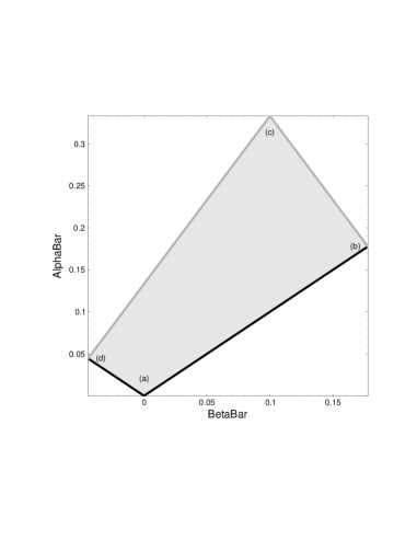
Figure 10: Bounds on ${\bar{\alpha}}$ and ${\bar{\beta}}$ for ${\bar{\pi}}=1/5$ and ${\bar{\varepsilon}}=1/3$, and the coordinates of the vertices given as general functions of ${\bar{\varepsilon}}$ and ${\bar{\pi}}$.

           

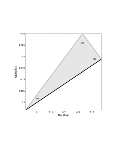
Figure 11: Bounds on ${\bar{\alpha}}$ and ${\bar{\beta}}$ for ${\bar{\pi}}=1/3$ and ${\bar{\varepsilon}}=1/4$, and the coordinates of the vertices given as general functions of ${\bar{\varepsilon}}$ and ${\bar{\pi}}$.

           

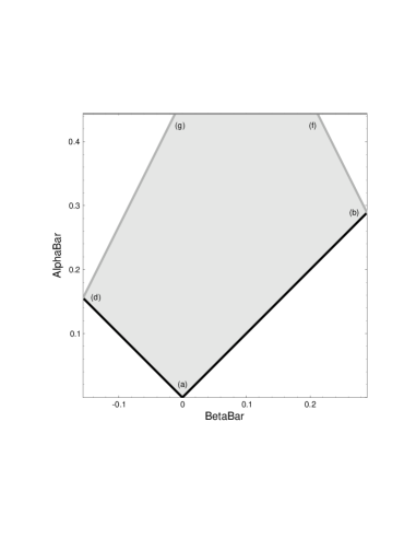
Figure 12: Bounds on ${\bar{\alpha}}$ and ${\bar{\beta}}$ for ${\bar{\pi}}=1/5$ and ${\bar{\varepsilon}}=2/3$, and the coordinates of the vertices given as general functions of ${\bar{\varepsilon}}$ and ${\bar{\pi}}$.

           

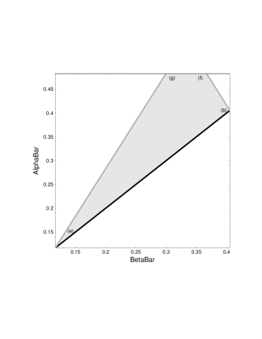
Figure 13: Bounds on ${\bar{\alpha}}$ and ${\bar{\beta}}$ for ${\bar{\pi}}=2/3$ and ${\bar{\varepsilon}}=11/20$, and the coordinates of the vertices given as general functions of ${\bar{\varepsilon}}$ and ${\bar{\pi}}$.

           

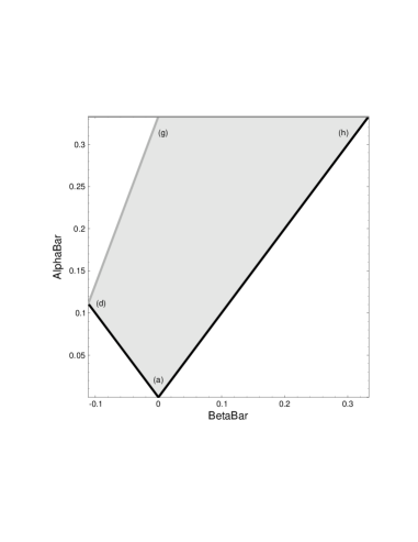
Figure 14: Bounds on ${\bar{\alpha}}$ and ${\bar{\beta}}$ for ${\bar{\pi}}=2/3$ and ${\bar{\varepsilon}}=1$, and the coordinates of the vertices given as general functions of ${\bar{\varepsilon}}$ and ${\bar{\pi}}$.

           

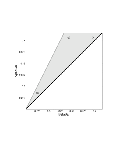
Figure 15: Bounds on ${\bar{\alpha}}$ and ${\bar{\beta}}$ for ${\bar{\pi}}=1$ and ${\bar{\varepsilon}}=3/4$, and the coordinates of the vertices given as general functions of ${\bar{\varepsilon}}$ and ${\bar{\pi}}$.

           

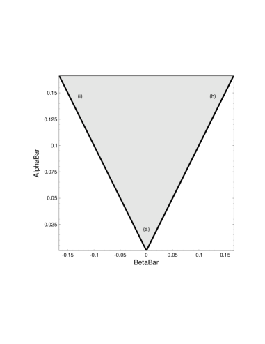
Figure 16: Bounds on ${\bar{\alpha}}$ and ${\bar{\beta}}$ for ${\bar{\pi}}=1/2$ and ${\bar{\varepsilon}}=3/2$, and the coordinates of the vertices given as general functions of ${\bar{\varepsilon}}$ and ${\bar{\pi}}$.

Appendix B Basis Bras and Kets for FCHC Model

In this appendix, we present one possible choice for the bras and kets of the FCHC model for three-dimensional fluid dynamics. The basis bras are shown in Table 4, and the basis kets are shown in Table 5.

$\left(\begin{array}[]{rrrrrrrrrrrrrrrrrr}1&1&1&1&2&2&1&1&1&1&2&2&1&1&1&1&2&2\\ 1&1&-1&-1&0&0&1&1&-1&-1&0&0&0&0&0&0&2&-2\\ 1&-1&1&-1&0&0&0&0&0&0&2&-2&1&1&-1&-1&0&0\\ 0&0&0&0&2&-2&1&-1&1&-1&0&0&1&-1&1&-1&0&0\\ \hline\cr 1&1&1&1&1&1&1&1&1&-1&-1&-1&-1&-1&-1&-1&-1&-1\\ -1&1&1&1&1&1&1&1&1&1&-1&-1&-1&-1&-1&-1&-1&-1\\ 1&1&1&1&1&1&-1&-1&-1&-1&-1&-1&1&1&1&1&1&1\\ 1&1&1&1&1&1&1&-1&-1&-1&-1&-1&-1&1&1&1&1&1\\ 1&1&1&1&1&1&1&1&-1&-1&-1&-1&-1&-1&1&1&1&1\\ 1&1&1&1&1&1&1&1&1&-1&-1&-1&-1&-1&-1&1&1&1\\ 1&1&1&1&1&1&1&1&1&1&-1&-1&-1&-1&-1&-1&1&1\\ 1&1&1&1&1&1&1&1&1&1&1&-1&-1&-1&-1&-1&-1&1\\ 1&1&1&1&1&1&1&1&1&1&1&1&-1&-1&-1&-1&-1&-1\\ -1&1&1&1&1&1&1&1&1&1&1&1&1&-1&-1&-1&-1&-1\\ -1&-1&1&1&1&1&1&1&1&1&1&1&1&1&-1&-1&-1&-1\\ 1&1&1&-1&-1&-1&1&1&1&-1&-1&-1&1&1&1&-1&-1&-1\\ -1&1&1&1&-1&-1&-1&1&1&1&-1&-1&-1&1&1&1&-1&-1\\ 1&-1&1&-1&1&-1&1&-1&1&-1&1&-1&1&-1&1&-1&1&-1\end{array}\right)$

Table 4: Bras for the three-dimensional projection of the FCHC model. The first four rows are the hydrodynamic bras, and the last 14 present one choice for the kinetic bras.

$\frac{\mbox{\scriptsize$1$}}{\mbox{\scriptsize$48$}}\left(\begin{array}[]{rrrr|rrrrrrrrrrrrrr}-16&8&8&-16&8&8&-16&8&8&-16&8&8&-16&8&8&-16&8&8\\ 12&0&-24&12&0&0&12&0&0&12&0&-12&12&0&0&12&0&-12\\ -24&12&36&-24&12&-12&-24&12&-12&-24&12&12&-24&12&-12&-24&12&12\\ -6&6&6&-6&18&-18&-6&6&-6&-6&0&6&-6&6&-6&-6&0&6\\ -36&12&12&12&-12&12&-36&12&12&-60&24&12&-36&12&12&-60&24&12\\ 0&0&0&-48&36&12&0&0&0&24&-18&-6&0&0&0&24&-18&-6\\ 29&-7&-19&5&11&5&5&-7&-1&29&-16&-13&29&-7&-1&29&-16&-13\\ -14&10&10&10&-14&-2&10&-14&-2&-14&10&4&-14&10&-2&-14&10&4\\ -6&-6&18&-6&6&-6&-6&18&-18&-6&0&6&-6&-6&6&-6&0&6\\ 18&-6&-6&-6&6&-6&18&-6&6&18&-12&-6&18&-6&-18&42&-12&-6\\ -9&3&15&15&-15&-9&-9&3&-3&-9&0&9&-9&3&-3&-33&24&9\\ 36&-12&-60&36&-12&12&36&-12&12&36&0&-36&36&-12&12&36&-24&-12\\ 22&-2&22&-26&22&-14&-2&-2&-14&22&-14&16&-2&-2&-14&22&-14&-8\\ -28&20&20&20&-28&-4&-4&-4&-4&-28&20&8&-4&-4&-4&-28&20&8\\ 24&-24&-24&24&0&0&24&0&0&24&-12&-12&24&0&0&24&-12&-12\\ 12&0&0&-12&0&0&12&0&0&12&-12&0&12&0&0&12&-12&0\\ -8&4&4&16&-8&-8&-8&4&4&-8&10&-2&-8&4&4&-8&10&-2\\ 12&-12&-12&12&-12&12&12&-12&12&12&0&-12&12&-12&12&12&0&-12\end{array}\right)$

Table 5: Kets for the three-dimensional projection of the FCHC model, corresponding to the choice of bras in Table 4. The first four columns are the hydrodynamic kets, and the last 14 are the kinetic kets.

References

- [1] U. Frisch, B. Hasslacher, and Y. Pomeau, Phys. Rev. Lett. 56 1505 (1986).
- [2] S. Wolfram, J. Stat. Phys. 45, 471 (1986).
- [3] U. Frisch et al., Complex Syst. 1, 648 (1987).
- [4] D.H. Rothman and S. Zaleski, Lattice-Gas Automata: Simple Models of Complex Hydrodynamics, (Cambridge University Press, 1997).
- [5] Hénon, M., Complex Systems 1 (1987) 763.
- [6] See, e.g., B.M. Boghosian, P.V. Coveney, and A.N. Emerton, Proc. R. Soc. Lond. A, 452, 1221 (1996); and B.M. Boghosian, P.V. Coveney and P.J. Love, “Three-dimensional lattice-gas model for amphiphilic fluid dynamics”, Proc. R. Soc. London A, in press (1999).
- [7] F. Higuera and J. Jimenez, Europhys. Lett. 9 (1989) 663.
- [8] F. Higuera, S. Succi and R. Benzi,, Europhys. Lett. 9 (1989) 345.
- [9] G. McNamara and G. Zanetti, Phys. Rev. Lett. 61 (1989) 2332.
- [10] S. Succi, R. Benzi, F. Higuera, Physica D 47 (1991) 219-230.
- [11] R. Benzi, S. Succi, and M. Vergassola Phys. Rep., 222 145 (1992).
- [12] E. Gross, D. Bhatnager, M. Krook, Phys. Rev. 94 (1954) 511.
- [13] Y.-H. Qian, D. d’Humières, P. Lallemand, Europhys. Lett. 17 (1992) 479-484.
- [14] A. Renda, G. Bella, S. Succi, I.V. Karlin, Europhys. Lett. 41 (1998) 279-283.
- [15] B.M. Boghosian, P.V. Coveney, Comp. Phys. Comm. (to appear, 2000).
- [16] Shan, X., Chen, H., Phys. Rev. E 47 (1993) 1815-1819.
- [17] Swift, M.R., Osborn, W.R., Yeomans, J.M., Phys. Rev. Lett. 75 (1995) 830-833; Swift, M.R., Orlandini, S.E., Osborn, W.R., Yeomans, J.M., Phys. Rev. E 54 (1996) 5041-5052.
- [18] N. Martys, Int. J. Mod. Phys. C 10 (1999) 1367-1382.
- [19] D. d’Humières, AIAA Rarefied Gas Dynamics: Theory and Applications, in Progress in Astronautics and Aeronautics 159 (1992) 450-458.
- [20] M. Schechter, Amer. Math. Monthly 105 (March, 1998) 246-251.
- [21] A.J. Wagner, Europhys. Lett. 44 (1998) 144-149.
- [22] I.V. Karlin, A. Ferrante and H.C. Öttinger, Europhys. Lett. 47 (1999) 182-188.
- [23] H. Chen and C. Teixeira, “H-theorem and Origins of Instability in Thermal Lattice Boltzmann Models,” preprint (1999).
- [24] R. Courant, K. Friedrichs, H. Lewy, Math. Ann. 100 (1928) 32.
- [25] J. Crank, P. Nicolson, Proc. Camb. Phil. Soc. 43 (1947) 50-67.
- [26] D.W. Peaceman, H.H. Rachford Jr., J. Soc. Ind. Appl. Math. 3 (1955) 28.
- [27] E.C. DuFort, S.P. Frankel, Math. Tables Aids Comput. 7 (1953) 135-152.
- [28] See, for example, B.M. Boghosian, “The Chapman-Enskog Method for Lattice Gases,” in 1989 Lectures in Complex Systems, Santa Fe Institute, E. Jen, ed. (1989).
- [29] G.R. McNamara, A.L. Garcia, B.J. Alder, J. Stat. Phys. 87 (1997) 1111-1121.
- [30] F.J. Alexander, A.L. Garcia, B.J. Alder, Phys. Rev. Lett. 74 (1995) 5212-5215.
- [31] B.M. Boghosian, P.V. Coveney, Int. J. Mod. Phys. 9 (1998) 1231-1246.
- [32] I. Karlin, Phys. Rev. Lett. 81 (1998) 6.
- [33] B.M. Boghosian, S. Succi, work in progress.