Two-dimensional hydrodynamic lattice-gas simulations of binary immiscible and ternary amphiphilic fluid flow through porous media

Abstract

The behaviour of two dimensional binary and ternary amphiphilic fluids under flow conditions is investigated using a hydrodynamic lattice gas model. After the validation of the model in simple cases (Poiseuille flow, Darcy’s law for single component fluids), attention is focussed on the properties of binary immiscible fluids in porous media. An extension of Darcy’s law which explicitly admits a viscous coupling between the fluids is verified, and evidence of capillary effects are described. The influence of a third component, namely surfactant, is studied in the same context.
Invasion simulations have also been performed. The effect of the applied force on the invasion process is reported. As the forcing level increases, the invasion process becomes faster and the residual oil saturation decreases. The introduction of surfactant in the invading phase during imbibition produces new phenomena, including emulsification and micellisation. At very low fluid forcing levels, this leads to the production of a low-resistance gel, which then slows down the progress of the invading fluid. At long times (beyond the water percolation threshold), the concentration of remaining oil within the porous medium is lowered by the action of surfactant, thus enhancing oil recovery. On the other hand, the introduction of surfactant in the invading phase during drainage simulations slows down the invasion process - the invading fluid takes a more tortuous path to invade the porous medium - and reduces the oil recovery (the residual oil saturation increases).

1 Introduction

Since the ability of lattice gas automaton (LGA) models to reproduce correctly the incompressible Navier-Stokes equations was established [1, 2], these models have been intensively studied. Rothman and Keller developed an extension of the one-component model for simulating binary immiscible fluids [3]. The introduction of a third component, namely surfactant, is due to Boghosian et al. [4]. The surfactant particle acts as a point dipole, and tends to stay at the interface between the two immiscible fluids. It can also form micelles, when its concentration exceeds a particular value (the critical micelle concentration). This work logically follows the two dimensional studies performed by Wilson and Coveney on flowing multiphase fluids, including their application to porous media [7]. Some preliminary results have been described in a first publication [9]. Complex fluid flow in porous media is both a scientifically challenging problem and a field of great practical importance, from oil and gas production to environmental issues in ground state water flows [10].
The paper is structured as follow: a short description of the hydrodynamic lattice gas model is given in Section 2. We present in Section 3 the results obtained for the simulation of single phase flow through a 2D channel and the verification of some theoretical predictions. These computations allow one to calculate the viscosity of the fluid. Section 4 is devoted to the verification of Darcy’s law and to its generalisation to the case of multiphase fluids. Invasion phenomena are investigated in Sections 5 and 6 and conclusions are presented in Section 7.

2 Description of the model

According to the lattice gas model for microemulsions [4], the sitewise interaction energy of the system can be written:

$$\Delta H_{int}=\alpha\Delta H_{cc}+\mu\Delta H_{cd}+\epsilon\Delta H_{dc}+\zeta\Delta H_{dd}.$$ (1)

These terms correspond respectively to the relative immiscibility of oil and water, the tendency of surrounding dipoles to bend round oil or water particles and clusters, the propensity of surfactant molecules to align across oil-water interfaces and a contribution from pairwise interactions between surfactant.
The use of a probabilistic, or Monte Carlo process, to choose the outgoing state when particles collide leads to the introduction of a temperature-like parameter $\beta$, which is, however, not related to a true thermodynamic temperature. This parameter does not allow the analytical prediction of the viscosity. In essentially all such lattice-gas models involving interactions between multicomponent species, the condition of detailed balance is not satisfied. This leads to the fact that one cannot be sure, a priori, that an equilibrium state exists. Nevertheless, numerical simulations confirm that steady states are reached. In this paper, the following set of parameters have been used:

$\alpha$	=	$1.0$
$\mu$	=	$0.001$
$\epsilon$	=	$8.0$
$\zeta$	=	$0.005$
$\beta$	=	$1.0$

We make use of a triangular (FHP) lattice, with six directions at each site. There can be up to seven particles at each site. The reduced density of a fluid phase is defined as the average number of particles of this fluid phase (colour) per lattice site, divided by $7$ (six lattice directions and one rest particle). Note that all simulations performed in this paper are two dimensional. A three dimensional version of the model has been formulated [5] and similar investigations are already underway using this high performance computing code [6]. The different fluid forcing methods are described in a previous paper [9].
Lattice sites are selected at random, on which momentum is added, so that either (a) the total average momentum is kept constant (“pressure” condition), or (b) the total added momentum is constant (“gravity” condition). In order to study the process of fluid invasion into porous media, some modifications have been made to our existing lattice-gas code [9]: The simulation cell system is no longer periodic in the flow direction (the vertical or y-direction), but retains periodicity in the x-transverse direction. To achieve this, “invisible” rows at the top and the bottom of the lattice have been added in order to simulate infinite columns of bulk oil and water respectively. As the total number of particles is conserved, they are wrapped from top to bottom and vice versa, but in so doing, they change their colour to that of the bulk surrounding colour fluid. When obstacle sites are present in the lattice, no-slip boundary conditions are used, corresponding to a zero velocity condition at the boundary in a conventional Navier-Stokes fluid. Obstacles may be given a colour charge, thus assigning wettability properties to the simulated rock species. The wettability index can vary over the range $\{-7;+7\}$, $-7$ corresponding to a rock site full of water (blue) particles, $+7$ to a rock site full of oil (red) particles (i.e. maximally hydrophilic and hydrophobic respectively).

3 Two-dimensional channel simulations

3.1 Single phase fluids

In this section, we first check some basic properties of single phase flow within channels in two dimensions, and then move on to consider binary immiscible fluid flow.

3.1.1 Velocity profile measurements

We are concerned here with the flow of a single phase fluid through a pipe (Poiseuille flow); the velocity profile in this case is known to be parabolic. The results obtained using a $32\times 32$ lattice are displayed figure 1. Also shown is a parabolic fit to the curve. The agreement between the simulated curve and the fit is good.

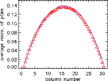
Figure 1: Velocity profile averaged over 20000 timesteps for a reduced density of 0.5 on a $32\times 32$ lattice. The simulated points are represented by triangles and the fitted curve is the dotted line. The forcing level is 0.00075 using gravity conditions.

This lattice gas model is able to reproduce correctly the flow of a single phase fluid through a pipe. The velocity profiles for low-density fluids (0-2 particles per lattice site) are less well-fitted by a parabola.

3.1.2 Calculation of the viscosity

From the velocity profile, we can extract the numerical value of the maximum flow velocity which occurs in the centre of the pipe. The relation between the velocity at the center of the pipe and the kinematic viscosity is:

$$\nu=\frac{1}{8}\frac{FW}{Lg_{max}},$$ (2)

where $\nu$ is the kinematic viscosity, $F$ is the forcing level, $W$ and $L$ are the width and the length of the channel respectively and $g_{max}$ is the maximum of the velocity in the center of the pipe. Carrying out this calculation for different densities allow us to compute the viscosity of the fluid as a function of density (figure 2).

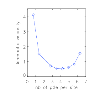
Figure 2: Kinematic viscosity as a function of density for a $32\times 32$ box size.

The result obtained with this model is in the same range as that obtained by Kadanoff et al. [8].

3.2 Binary immiscible fluid flow in a channel

Simulations of binary mixtures in a two-dimensional pipe were conducted on a $32\times 128$ lattice. The first set of simulations concerned the influence of the wettability index on the shape of a non-wetting fluid bubble and the second set involved a study of the coupling between the two fluids.

3.2.1 Influence of the wall wettability

In order to study the effect of the wettability index on the shape of a non-wetting bubble, invasion conditions are used. These conditions simulate infinite columns of wetting and non-wetting fluid at the top and the bottom of the lattice respectively, thus allowing the non-wetting bubble to adhere to the walls (at least at the bottom of the lattice). If the simulations are performed without bulk flow, the wetting phase progressively invades the lattice (owing to capillary effects), preventing a detailed study of the non-wetting bubble. The simulations are run using pressure forcing applied to the non-wetting fluid, in order to achieve a state of zero flux (momentum is added to the non-wetting phase until its flux reaches a zero value). The force needed to keep the non-wetting fluid on the lattice is then determined, as a function of the wettability of the walls. Figure 3 displays the results for a 1:1 water and oil mixture with a total reduced density of either 0.5 or 0.7. Each point is averaged over 5 independent simulations, each of duration $20000$ timesteps.

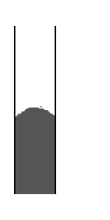
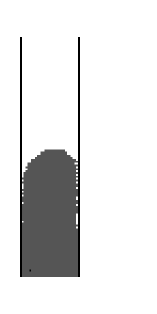
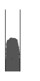
Figure 3: Effect of the wettability index on the force needed to keep the non-wetting fluid on the lattice. The curves with diamonds and triangles correspond to reduced densities of $0.35$ and $0.25$ respectively. The configurations from left to right correspond to simulations with wettability $0$, $1$, $2$, and $3$ (the wetting fluid is in white). The force is in unit momentum per timestep and the lattice size is $32\times 128$.

Several points can be made. First of all, the curves corresponding to different reduced densities are similar. They display a strong influence of the wettability index in the range $0-3$, for which the force needed to keep the non-wetting fluid on the lattice increases strongly. For wettability indices greater than $3$, there is no change in the restraining force. Snapshots at different times during the simulation show that for non-wetting walls, the interface is on average flat. Increasing the wettability leads to deformation of the interface, from a flat to a curved interface, and finally to the detachment from the wall of the upper part of the non-wetting bubble, for an index of $2$. Increasing the wettability index further has no effect because the bubble has already detached from the wall.
It is surprising that the reduced densities of the fluids do not influence this curve. One might have thought that the point at which the bubble detaches from the wall would correspond to there being an equal number of particles per site in the wetting fluid and in the obstacle sites so that, when the reduced density of the wetting fluid increases, the bubble would detach for greater wettability coefficients, but this is not found to be the case.

3.2.2 Coupling

The coupling between the two fluids is studied here. In these simulations, only one fluid is forced, and the response of both fluids (forced and unforced) is calculated, for different applied forces. The results are plotted in figure 4. Simulations were performed over $20000$ timesteps, with a reduced density of $0.25$ for each fluid. The wettability of the wall is $-7$, i.e. strongly water-wetting.

Figure 4: Response of fluids when they are either force (left) or unforced (right). Stars and diamonds are for oil and water respectively. The normalised force is the force divided by the force at which linear behaviour first arises. The normalised flux is the flux divided by the flux of a single component fluid at that forcing.

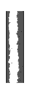
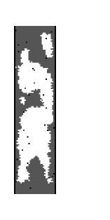
Figure 5: A configuration showing the oil phase (white) as a single bubble (low forcing), a continuous phase (intermediate forcing) or disconnected phase (high forcing). The velocity profiles, averaged over 10000 timesteps, correspond to a continuous oil phase when either oil (left) or water (right) is forced. The lattice size is $32\times 128$.

The behaviour of the two fluids when they are forced is different. The curve associated with water lies below the one for the oil because of the wettability of the wall. At small oil forcing levels, the oil phase exists as a single elongated bubble, and its response is non-linear. When the force becomes large enough, the response of oil becomes linear. For an applied force greater than $2$ normalised units, a discontinuity is seen, which corresponds to the formation of an infinite lamellar phase (the bubble now extends over the whole lattice). In this regime, the response of oil is still linear. At very high forcing levels, the response again becomes non-linear. This is presumably due to the limitation in fluid velocity of the spatially discrete lattice gas model.
By contrast, the response of water is linear from the smallest forcing levels to a force of approximately $2$ normalised units (figure 4). The breakpoint at this forcing level corresponds, as in the case of the forcing of oil, to the formation of a continuous infinite oil phase. In this regime, the response is still approximately linear. Increasing the water forcing level leads to the break up of this infinite oil phase into several oil droplets, which are no longer ellipsoidal in shape.
On the other hand, the response of both fluids is identical when they are unforced but driven by coupling to the forced second phase: linear behaviour is observed for a forcing level up to $2$ normalised units. For higher forces, the response is roughly linear, albeit a little lower than before, due to the formation of a continuous oil phase.
Figure 5 illustrates the different behaviour observed. On the velocity profile corresponding to a continuous oil phase when water is forced, a parabolic profile can be discerned on the right hand portion of the plot (where water occupies the lattice) while a linear segment on the left hand side corresponds to the location of the oil, which behaves as if it were under shear (couette) conditions. When oil is forced, the central and left hand part of the velocity profile is parabolic (Poiseuille flow for the central oil phase) while the linear behaviour is associated with the location of water at each side of the channel, under conditions approximating couette flow.

Figure 6: Dependence of fluid flow on fluid composition as a function of wall wettability for progressively less water-wetting channel walls; the wettability index has the numerical value $-7$ (crosses), $-2$ (squares), $-1$ (diamonds) and $0$ (stars). The normalised momentum is the momentum divided by the momentum of a pure fluid at the same level of forcing. Data are averaged over 10000 timesteps on a $32\times 128$ lattice. For clarity, error bars are displayed only for one set of simulations.

Figure 6 displays the results of the calculation of the relative permeability coefficients over the whole range of water concentration, and for different channel wettability indices. In the case where oil is forced, the plots of the oil response become more curved as the wettability of the wall increases ( the curve is convex up to $0.4-0.5$ water concentration, and concave for higher concentrations). Moreover, lubrication effects are seen at small water concentrations, and they become more important as the wettability coefficient increases (lubrication is manifested by a normalised momentum greater than one). This is due to the fact that when the wettability coefficient is small (between $0$ and $2$), the water preferentially accumulates at only one side of the walls. Thus the oil is in direct contact with the other wall. For the highest wettability index (-7), the water adheres to both sides, and the oil flows in the centre of the pipe, avoiding any contact with the walls. Thus the oil does not dissipate momentum on the wall anymore, and the resulting flow is greater than that of a pure fluid.
By contrast, when water is forced, the concavity of the flux-composition curves increases with the wettability index, and the curves remain concave over the whole composition range.
The main effect of increasing the wettability index on the response of unforced fluids is that the viscous coupling between the two fluids then also increases. Moreover, a secondary maximum appears, when the wettability decreases (in the case of unforced oil at low water concentration) or increases (in the case of unforced water at high water concentration). In the latter case, this peak is related to the fact that at very high water concentration, there is a small (roughly spherical) oil bubble which can flow in the pipe (whose diameter is lower than the diameter of the pipe). When the water concentration decreases, the diameter of the oil bubble increases and becomes identical to the diameter of the pipe, at which point it experiences direct interaction with the wall. In the case of unforced oil, the secondary maximum is associated with the formation of water droplets rather than elongated layers along each wall. These droplets can flow easily, and the resulting coupling with water is enhanced. As in the case of forced fluids, the main effect of the wettability index appears in the range $0-2$.

4 Darcy’s law and its generalisations

In this section, we are concerned with the study of fluid flow in porous media. The first sub-section describes the method used to construct a porous medium, which differs from the random distribution of obstacle sites used previously [9]. In the case of a single component fluid, the validity of Darcy’s law is investigated, for various porous media. In the case of binary immiscible fluids, there is no generally accepted law governing the flow behaviour of the mixture. A generalisation of Darcy’s law (eq 5) is used in previous work, which explicitly admits viscous coupling between the two fluids. The importance of this coupling is examined for various porous media. The dependence of fluid flow on the fluid composition is investigated. Finally, an investigation of the influence of surfactant is also presented.

4.1 A brief review

There have been a few studies concerning the calculation of relative permeabilities of two-phase flow in porous media. In two dimensions, Rothman [11] used a lattice-gas method to investigate the validity of macroscopic fluid flow laws in porous media. He constructed a porous medium comprised of a square block in the middle of a pipe. For each saturation, he computed the four phenomenological coefficients (see equation 5) from the slope of the linear response of the flux (of each species) to the applied force. He then constructed a relative permeability diagram, which shows that the viscous coupling is not negligible (typically of the order of $0.2$ for a $50\%$ saturation). Nevertheless, his model “porous medium” was extremely simple. Kalaydjian [12] compared theoretical predictions with experimental results on the behaviour of an oil ganglion in a capillary tube square cross section and axial constriction. He found that for a ratio of viscosities equal to one, the effect of viscous coupling is significant. Moreover, taking into account variation of the viscosity ratio of the two fluids, the relative permeability can assume values greater than one, indicative of lubrication effects. Goode and Ramakrishnan [15], have calculated relative permeabilities in the case of a tube network using a finite element method. They found that the viscous coupling is very small. They also studied the influence of the viscosity ratio on lubrication. Zarcone et al. [14] have constructed an experimental setup to determine the coupling coefficient from a single experiment. The porous medium was a packing of sand grains and the experiments were performed on pairs of fluids (mercury/water and oil/water). They assumed that the cross-coefficients were equal over the whole range of saturation and found that they could be neglected in both cases. In a recent study, Olson and Rothman [13] have calculated relative permeabilities using the lattice-gas method in three dimensions, for a digitized microtomographic image of Fontainebleau sandstone. The coupling coefficients appear to be very small and Onsager’s reciprocity relation is verified.

4.2 Construction of two-dimensional porous media

It is known that the behaviour of fluids in porous media changes dramatically when going from 2D to 3D and it is frequently stated that there is no such thing as a porous medium in two dimensions. Nevertheless, 2D simulations can be compared to 2D-like micromodel experiments, and prove to be helpful in understanding this complex problem. The first step needed before doing any simulation is the construction of a porous medium itself. If we take a 2D slice of a 3D porous medium, we cannot be sure that the pores are connected (the connection may appear in the third dimension), and thus simulations in such media would be impractical. On the other hand, a regular porous medium can introduce unwanted symmetry and thus introduces artifacts into the results.
The method used by Wilson and Coveney [7] to create a porous medium consists of randomly placing obstacle sites on the lattice. This has the disadvantage that the resulting medium has rather uncontrollable properties. The method proposed here ensures control of the size and dispersion of solid obstacles without imposing any symmetry: first a simulation of domain growth in an oil-water binary mixture is run, starting from a random configuration. The temporal evolution of such a mixture is marked by the formation of small droplets of oil in bulk water [4]. These droplets coalesce with each other, becoming larger and larger. When the size of the droplets reaches the desired size for the obstacle, the simulation is stopped and the oil sites are stored as obstacle sites for latter use. Figure 7 shows examples of porous media constructed in this way, which have been extensively used in the simulations described here.

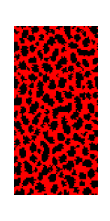
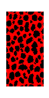
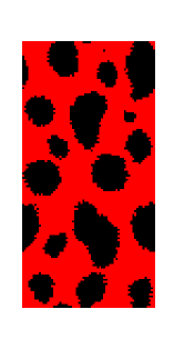
Figure 7: Examples of porous media ($64\times 128$ lattice sites) constructed from domain growth in a binary phase. Obstacle sites are coloured in black. (right): small, (center) medium, (left) large.

One should note that the porosities of these media are roughly equal to each other (table 1); the differences originate from the average size of the obstacle grains. The use of these kinds of porous media enables us to readily change the scale of the simulations.

Table 1: Properties of the three porous media (small, medium and large) shown in figure 7. The effective surface is the number of available lattice sites in direct contact with an obstacle site. A site is far from an obstacle if the distance to the nearest obstacle site is larger than one lattice site.

Properties	Small	Medium	Large
Porosity	$55\%$	$52\%$	$60\%$
Number of available sites	$4466$	$4230$	$4929$
Effective surface	$3288$	$2407$	$1101$
Number of sites far from obstacle	$1178$	$1823$	$3828$

4.3 Single phase fluids

In the case of single component fluids, the flow is governed by Darcy’s law:

$$\mathbf{J}=-\frac{k}{\mu}(\mathbf{\nabla}p-\rho\mathbf{g})$$ (3)

where $\mathbf{J}$ is the flux, $k$ the permeability, $\mu$ the kinematic viscosity, $\mathbf{\nabla}p$ the pressure gradient and $\rho\mathbf{g}$ the gravitational force density. To determine permeabilities for these three porous media, simulations were performed at a reduced density of 0.6 particles per lattice direction with an initially random configuration. The flux was averaged over the entire lattice and over 7500 timestep intervals, after the flow had reached a steady state. Figure 8 displays the results calculated over a wide range of applied forces, making use of the gravity condition.

Figure 8: Verification of Darcy’s law for a single component fluid in the three different porous media of table 1 and 7. The lines are linear fits to the data. Triangles, crosses and diamonds refer to the large, medium and small porous media respectively.

In the three porous media (cf table 1), a linear expression fits the simulated points: Darcy’s law is thus obeyed in these cases. However, for very high levels of forcing, nonlinear effects appear (for the largest porous medium). The slope of the linear fit is proportional to the permeability of the porous medium; the ratios of these slopes are reported in table 2.

Table 2: Ratios of the permeabilities ($k_{s},k_{m},k_{l}$) of the small, medium, and large porous media respectively.

Ratio of permeabilities	$\frac{k_{m}}{k_{s}}$	$\frac{k_{l}}{k_{m}}$	$\frac{k_{l}}{k_{s}}$
Numerical value	$1.8$	$8.5$	$15.7$

All these simulations were performed under the same conditions: the viscosity of the fluids is unchanged and the porosities of the various porous media are very similar to one another. The slopes of the lines, i.e. the permeabilities of these three porous media are strongly dependent on the chosen resolution (averaged number of lattice sites per pore).

4.4 Binary immiscible fluids

Even binary immiscible fluid flow in pipes is a problem for conventional continuum fluid dynamics methods, because of the complexity of the fluid interfaces, particularly at high Reynolds numbers. Similar challenges remain for the modelling and simulation of two-phase flow in porous media, even at very low Reynolds numbers.

4.4.1 Cross-coefficients and Onsager relations

At the outset, we should stress that there is no well-established law governing the flow of binary immiscible fluids through porous media. One might consider the simplest extension of Darcy’s law for two components of the form:

$$\mathbf{J_{i}}=k_{i}(S)\frac{k}{\mu_{i}}\mathbf{X_{i}},$$ (4)

where $\mathbf{J_{i}}$ is the flux of the $i$th species, $k_{i}$ is the relative permeability coefficient (depending on the saturation $S$), $\mu_{i}$ is the viscosity, and $\mathbf{X_{i}}$ is the body force acting on the $i$th component. These equations assume that the fluids are uncoupled (i.e. each fluid flows in a porous medium formed by original the porous medium plus the other fluid).
However, if we assume that the fluids are coupled, the generalised form of Darcy’s law becomes:

$$\mathbf{J_{i}}=\sum_{j}{L_{ij}\mathbf{X_{j}}},$$ (5)

where $i,j=1,2$. Eq 5 is a more general form of linear force-flux relationship. These equations have a similar structure to that which arises in the theory of linear irreversible thermodynamics. The coefficients $L_{ij}$ are then referred as to phenomenological coefficients. In this theory Onsager’s reciprocity relation applies (the cross coefficients are equal ($L_{12}=L_{21}$)). Tempting as it is, one must nevertheless be very careful about claiming that there is more than a formal similarity in this case. Onsager’s theory depends on various physical assumptions, such as detailed balance, which are obviously not satisfied here.
Simulations have been performed on a 1:1 mixture of water and oil, at a total reduced density of 0.5, using the three porous media described in table 1. The wettability index of the rock was set at $-7$ throughout. The applied force (gravity condition) varies over the range [0.0001, 0.2]. To calculate the different phenomenological coefficients, we computed the response of both fluids when each one is forced (figure 9).

Figure 9: Investigation of a generalised version of Darcy’s law: calculation of the phenomenological coefficients as the slope of the response of each fluid component when they are either forced (diagonal) or unforced (cross-coefficients) in the case of the small (top), medium (centre), and large (bottom) porous media of table 1. Oil and water are represented by stars and squares respectively. Data are averaged over 10000 timesteps on a $64\times 128$ lattice.

In the literature [13], the force is normalised with respect to the capillary threshold (the force needed for an oil bubble to flow). In our work, particularly using the small obstacle matrix, the flux of water becomes linear at higher forcing levels than for the oil. Thus the normalisation is made with respect to the appearance of a linear response for both fluids.
The response of forced fluids is linear over a large applied force range in the case of the small porous medium, and for low forces in the case of the large one. Thus we can extract the coefficients $L_{11}$ and $L_{22}$ from the slope of the linear regime. The coefficient relative to the water is lower than the one for the oil because of the wettability of the porous medium. The water preferentially adheres to the obstacles rather than flowing in the channels. However, the two diagonal coefficients have the same order of magnitude.
In the case of oil, capillary effects can be seen at very low forcing levels. This leads to non-linear behaviour. This non-linearity vanishes for applied forces greater than a critical value corresponding to the capillary threshold. In the case of water, the non-linearity disappears when the average size of the channels increases (that is, for the large porous medium). When the channels are very narrow, a small oil bubble can easily block the flow of water. Thus, this non-linearity is directly related to the width of the channel; it may also be influenced by the connectivity of the obstacle matrix (tests have been made to check the influence of the bounce-back (no-slip) boundary conditions at obstacles on this behaviour. It appears that using other types of conditions does not change these results).

The behaviour of the unforced fluids is quite different: in the case of oil, the response is linear, even for small applied forces. This is presumably due to the fact that oil particles reside preferentially far from obstacles and so a flux of water particles will necessarily induce a flux of oil particles. In the case of unforced water, its response is linear only if the applied force is greater than a critical value (in the small and medium sized porous media). In the low forcing regime, the response is clearly non-linear and sometimes even negative. This non-linearity can be attributed to the wettability of obstacles with respect to water as well as to the fact that oil bubbles can block pore throats and so prevent the flow of water.
However, the cross-coefficients in the generalised form of Darcy’s law (eq. 5) are nearly equal to each other (figure 9). The surprising thing is that the numerical values of the cross coefficients are of the same order of magnitude as those of the diagonal coefficients $L_{11}$ or $L_{22}$. In comparison with the results obtained by Rothman et al [10], this fact may be attributed to the dimensionality of the model (we are working in 2D while  [10] is concerned with the 3D case) and to the porous media used. The relative permeabilities are reported in table 3 for each porous medium.

Table 3: Relative permeabilities for the three porous media of table 1, and coupling cross-coefficients. Their ratios are also reported. Indices 1 and 2 refer to oil and water respectively.

$\mathbf{Obstacle}$	$\mathbf{Small}$	$\mathbf{Medium}$	$\mathbf{Large}$
$L_{11}$	$0.27$	$0.38$	$0.42$
$L_{22}$	$0.09$	$0.12$	$0.17$
$L_{12}$	$0.17$	$0.15$	$0.14$
$L_{21}$	$0.17$	$0.16$	$0.12$
$\frac{L_{11}}{L_{22}}$	$3.0$	$3.17$	$2.47$
$\frac{L_{12}}{L_{21}}$	$1.0$	$0.94$	$1.17$
$\frac{L_{11}}{L_{12}}$	$1.59$	$2.53$	$3.0$
$\frac{L_{22}}{L_{21}}$	$0.53$	$0.75$	$1.42$

The increase of the relative permeabilities when going from the small to the large porous medium can be understood in term of connectivity of space: in the case of the small porous medium, pores are numerous and very small, and the oil phase is much more disconnected than in the large obstacle matrix, in which the pores are large, enabling the oil to form larger droplets. Thus the amount of fluid-fluid interface decreases when going from the small to the large porous medium. This explains the small decrease of the cross coefficients and the increase of the relative permeabilities of each fluid.
Note that the ratio of cross terms is approximately constant, and equal to one. This supports the notion of Onsager reciprocity, which seems to be valid in spite of the fact that various properties, such as detailed balance, are not maintained by the lattice gas model. Moreover, the ratio of diagonal terms is also approximately constant, implying that a correlation exists between the forcing of oil and water. Nevertheless, the ratio of diagonal to off-diagonal terms for each fluid is not constant: this is due to the fact that the coupling between the two fluids also depends on the geometry of the porous medium.
These simulations demonstrate that there is significant coupling between the two fluids, at least in the case of these particular porous media. This strong viscous coupling is thought to be due to the dimensionality of the model. The reciprocity relations seem to be valid over a well-defined range of applied forces, and the response of the fluids remains linear down to a well defined value of the applied force.

4.4.2 Relative permeabilities as a function of saturation

In the last section, we calculated the cross-coefficients in a linear generalisation of Darcy’s law in various porous media. These results were obtained by looking at the response of each fluid when they are either forced or unforced, for different applied forces. We focus now on the behaviour of fluids for different water saturations. For this study, a new porous medium was selected (see figure 10), because of its large connectivity. For each saturation, the flux of each fluid is calculated when it is forced or unforced. The results are shown in figure 10. These curves have been calculated taking into account only the flux of majority colour sites, but the results are identical if the total flux of particles is considered. The wettability of the porous medium has been set equal to $-7$. The total reduced density is 0.7 and the forcing level is 0.005 (gravity condition). Also shown in figure 10 is the coloured velocity profile in the porous medium considered.

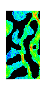
Figure 10: Left: binary immiscible fluid flow behaviour as a function of water saturation. The normalised momentum is the total vertical momentum divided by the total vertical momentum of pure fluid at the same forcing level in the same porous medium. Water is represented with crosses (forced) and stars (unforced) and oil with triangles (forced) and squares (unforced). Right: coloured velocity profile of the flow of a single phase fluid in the same porous medium. Red and blue are associated with large and low velocities respectively. The size of the porous medium is $64\times 128$. Averaging is performed over 10000 timesteps.

The behaviour of the two immiscible fluids when only water is forced is described first. At low water saturations, water particles form small bulk water clusters together with some isolated particles which adhere to the obstacle matrix. Some of the clusters flow through the channels while others are trapped in stagnant zero-velocity regions. When the water concentration increases, the cluster size grows, and the water still occupies both channel sites and stagnant regions. As the water concentration increases, there is no change in the sites occupied by water: the mechanism of flow is unchanged.
Consider now the behaviour of the oil when only water is forced. The coupling is maximum for $60\%$ water, corresponding to a significant water flux. When the water concentration increases, the oil flux decreases because there is less oil in the medium. Equally, when the water concentration decreases, the oil flux decreases because there is not enough water to drive oil. However, the case of forced oil is different. At low water saturation, the water still forms clusters as well as surrounding obstacles but now the clusters are all trapped in stagnant zero-velocity zones. The normalised flux of water is zero while the normalised flux of oil is greater than one. This means that a mixture of oil together with a small amount of water produces a larger flow than that of pure oil. This can be explained on the basis of a lubrication phenomenon, as in the case of a flowing binary immiscible fluid in a pipe (see section 3.2). As shown below, this is largely due to geometrical properties of the porous medium. When the water concentration increases, the oil still flows freely in the channels. Water clusters accumulate preferentially in stagnant zones. When the water concentration increases, the flux of the unforced water increases, for the same reasons as before. However, the decrease of the oil flux is associated with a reduction of the connectivity of the oil phase. At higher water concentrations, the flux of water decreases because of the decrease of the oil flux. The very small residual oil saturation is due to the use of random initial configurations: the results are different in invasion simulations (sections 5 and 6).

Figure 11: Binary immiscible fluid flow behaviour as a function of water concentration. The normalised flux is the total vertical momentum divided by the total vertical momentum of pure fluid at the same forcing level in the same medium. Water is represented with crosses (forced) and stars (unforced) and oil with squares (forced) and diamonds (unforced). The lower graph corresponds to a forcing level of $0.005$ while the upper one corresponds to a forcing of $0.001$.

The same calculations have been performed using the large porous medium described in table 1. The results are displayed in figure 11 (total density $0.7$, wettability coefficient $-7$, forcing levels $0.001$ and $0.005$, averaged over $10000$ timesteps). The two diagrams in figure 11 represent simulations in the same porous medium, but with forcing either greater or lower than the capillary threshold respectively. In the former case, the residual oil saturation is very small, and the effect of the connectivity of the oil phase is small. The cross-coefficients are roughly equal over a large range of fluid compositions and the viscous coupling between the two fluids is non-negligible. The role of the residual water concentration is significant, owing to the wettability of the rock and the connectivity of the obstacle matrix.
In the low forcing case (figure 11), the residual oil saturation is very high. The appearance of a non-zero oil flux is related to the connectivity of the oil phase: when oil exists only as bubbles, it cannot flow. The coupling between the two fluids is very small, because of the high residual saturations (the flux of the forced phase is zero, as is the flux of the unforced phase).
In both diagrams, lubrication phenomena are seen at very low water concentrations. Figure 12 displays the results obtained in the case of a porous medium comprising a single pore.

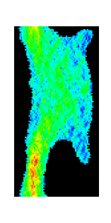
Figure 12: Left: binary immiscible fluid flow behaviour as a function of water concentration. No lubrication phenomenon is exhibited in this case. Water is represented with crosses (forced) and squares (unforced) and oil with triangles (forced) and diamonds (unforced). Error bars are also displayed. Right: the single pore porous medium used, together with a velocity profile; colour coding as in previous figures.

The principal result is that lubrication effects are not very important in this case. It therefore seems that lubrication effects in the other porous medium used are due to the topology of the obstacle matrix, being dependent on the amount of solid-liquid interface.
In summary, for binary immiscible fluid flow in porous media, it appears that when the forcing is greater than the capillary threshold, the shapes of the relative permeability curves agree well with what has been published previously concerning simulation results. The residual oil saturation is small, and is probably due to the topology of the porous medium and to the use of random initial configurations. The porous medium can also produce “lubrication” effects, at very small levels of water saturation. The coupling coefficients appear to be roughly equal over a large range of saturations, and exhibit a maximum of $0.2$ for $60\%$ water saturation. When the forcing is lower than the capillary threshold, the oil flux is strongly dependent on the connectivity of the oil phase.

4.5 Ternary amphiphilic fluids

In this section the effect of surfactant on the hydrodynamic behaviour of oil/water fluid mixtures in porous media is investigated. In the binary immiscible fluid case, the fluxes of the different species were normalised by the flux of a pure fluid in the same medium, of density equal to the sum of the partial densities. In the ternary case, the flux of each species is normalised by the flux of a pure fluid of density equal to the sum of the partial densities of oil and water.
The simulations are performed using the large (cf table 1) obstacle matrix. As in the binary case, the gravitational flow implementation is used. The reduced densities of oil and water are equal to $0.2$, and the reduced density for surfactant is set equal to $0.1$ (for this surfactant concentration, the equilibrium state without flow corresponds to the microemulsion phase). Results are displayed in figure 13.

Figure 13: Evolution of the response of fluids when they are either forced (left) or unforced (right), as a function of the forcing level, in the ternary amphiphilic case, and using the large porous medium (cf table 1). Water is represented with crosses (forced and unforced), oil with triangles (forced and unforced), surfactant with diamonds (oil forced) and squares (water forced).

As in the binary case, the response of fluids when they are forced is approximately linear, provided the applied force is greater than a threshold value, the capillary threshold. The diagonal coefficients (relative permeabilities) can then be calculated from the slopes of these lines. Their values are ${\it\kappa_{ww}}\approx 0.20$ and ${\it\kappa_{nn}}\approx 0.50$. The capillary threshold is lowered by a factor of $\approx 2$ (now equal to $0.0005$) in comparison with the binary case. This change is due to a lowering in surface tension (oil can now pass more easily through narrow channels).

5 Imbibition simulations

This work follows some initial studies done by Fowler and Coveney [16] on the invasion process in a porous medium. They used a randomly constructed porous medium made as described in [7] to study the effect of surfactant on the invasion process in the cases of drainage and imbibition. We have used the same type of porous media. In this section, we consider only the case of imbibition. The imbibition process refers to the invasion of a wetting fluid with or without surfactant into a porous medium filled with a non-wetting fluid. The aim of the following study is to characterise the invasion process, and to investigate the influence of surfactant on this process.

5.1 Invasion process

A typical result obtained from an invasion simulation, given in terms of the evolution of the number of particles of each species versus time, is displayed in figure 14.

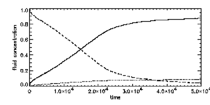
Figure 14: Variation of the number of oil (dashed line), water (continuous line) and surfactant (dot line) particles versus time when a water-wetting porous medium filled with oil is invaded by a mixture of water and surfactant. The porous medium is displayed in figure 19, and the lattice size is $128\times 256$. Data come from a single run.

This time evolution can be decomposed into two parts. In the first regime, at early times in the simulation, the change in the number of particles is roughly linear with time. The end of this regime corresponds to percolation of the water phase, that is breakthrough by the invading water phase. The second regime shows a slow variation of the number of particles of a given type with time, and a continuously connected path of the invading fluid exists across the lattice. In this domain a steady state has been reached. The number of particles of a given type tends slowly to an asymptotic value. This asymptote corresponds to the residual oil saturation. Figure 15 displays the gradient of the number of water particles versus time, or the water mass flux, for the simulation data shown in figure 14. The two regimes described above can be identified here more clearly. Prior to water percolation, the decrease in the number of oil particles is linear and its gradient is constant in time. After this period, the gradient assumes a small value, corresponding to the existence of a continuously connected pathway of the invading fluid across the lattice simulation cell.

Figure 15: Rate of change of water particles versus time (i.e. the water mass flux) for the simulation data shown in figure 14.

Between the two domains described above, there is a transient region, in which the gradient decreases from its constant finite value to zero. At the end of the first time interval, the water attains its percolation threshold. At the beginning of the second temporal domain, the flux of oil is very small and the oil forms only disconnected bubbles. In the transient regime between these two domains, both fluids are percolating and the flux of each species is non-zero. Oil particles are driven off the lattice while water occupies more and more sites. The end of the transient domain is associated with the end of oil percolation.

5.2 Effect of forcing

The effect of the applied force is investigated in the first steps of the invasion process, that is prior to the onset of water percolation. In this regime, the number of oil particles decreases linearly with time (the oil mass flux is essentially constant). Figure 16 displays the results obtained for the small porous medium (cf table 1), with no surfactant, for different applied forces. The simulations were performed over 75000 timesteps.

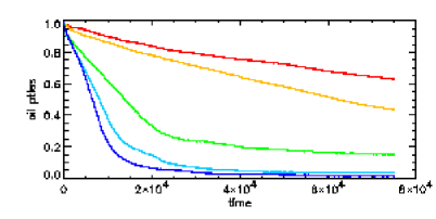
Figure 16: Invasion of water in a water-wetting porous medium filled with oil (imbibition), showing the effect of the applied force on the flux of oil particles. The time is the number of timesteps and the y-axis is the normalised number of oil particles in the lattice. The porous medium has dimensions $64\times 128$. Each curve is a result of a single simulation. Before percolation, the flux exhibits a linear dependence on time. The different forcing levels (from top to bottom) are 0.0005, 0.001, 0.005, 0.01, 0.025 (using gravity conditions).

A linear variation of the number of oil particles versus time before water percolation is observed. The slopes of these lines are calculated for different applied forces. This calculation was performed for several different porous media, and the results are collected in figure 17.

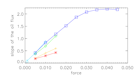
Figure 17: Effect of the applied force on the gradient of the flux of oil particles for porous media (randomly created and also built using the method described in section 4.2) of various size ($64\times 128$ and $128\times 256$). Each point is a result of a single simulation.

From these curves (calculated before the percolation threshold), we can see that there is a linear regime in the evolution of the oil flux. The oil flux is then directly proportional to the force applied to the water particles. Thus the greater the forcing on water, the faster the oil flows (and the sooner the percolation threshold is reached).
At very high forcing levels, the gradient of the oil flux no longer exhibits a linear dependence on the applied force but rather tends to an asymptotic limit. This behaviour is probably related to the limited velocity of the particles in the lattice gas model; otherwise, it would mean that an optimal value of the forcing level exists to maximise oil production, implying that the application of ever increasing forces will not be beneficial.

5.3 Effect of surfactant on imbibition

Emulsification

As Fowler and Coveney have noticed [16], one often encounters substantial variation in results for similar simulations. This means that precise results require substantial ensemble averaging, and so one must be very careful in attempting to draw conclusions from one or a limited number of simulations. Bearing this in mind, we start by a careful study of the effect of surfactant at the pore level. The porous medium is now composed of only one pore as shown in figure 12. This is obviously not representative of a porous medium but nevertheless it contributes to our understanding on what happens on larger scales. The conclusion arising from this particular porous medium is that the termination of oil percolation takes longer to occur in the case with surfactant, and hence that oil recovery is enhanced. The behaviour of the fluids after the end of oil percolation is strongly dependent on whether surfactant is absent or present. Without surfactant, the remaining oil forms large spherical droplets which can barely flow, whereas the presence of surfactant favours the formation of smaller oil droplets (the surfactant concentration required to achieve this is quite high, typically $0.2-0.3$), which can flow very easily. Therefore, in this example of imbibition, the introduction of surfactant strongly enhances oil recovery.
These phenomena observed at the pore level are also manifested at larger scales. Figure 18 displays configurations obtained when flooding a porous medium filled with oil by either water or a mixture of water and surfactant.

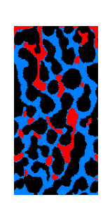
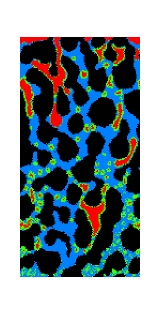
Figure 18: Configuration obtained during flooding a porous medium filled with oil by either water (left) or a mixture of water plus surfactant (right). The size of the lattice is $64\times 128$. The configurations are taken just before the end of oil percolation. The emulsification phenomenon can easily be seen in the latter case.

From this figure, we can see that when there is no surfactant, rather large oil droplets remain in the rock. On the other hand, in the presence of surfactant, a large number of small oil droplets can be seen surrounded by surfactant. These small droplets are less affected by capillary effects and can flow readily. However, we also notice that the concentration of surfactant is greater in the lower part of the box, from where the flooding occurred. There are two reasons for this: first, surfactant particles are rapidly trapped when they encounter the first oil-water interface. This trapping remains until the oil droplets form and flow. Second, surfactant particles can self-assemble into small clusters [17, 18], which can be trapped in small pores. This phenomenon, called micellisation, is discussed further below.
These various emulsification phenomena are clearly observed in our imbibition simulations, and tend to decrease the residual oil saturation in the steady state regime, thus improving the oil recovery.

Micellisation

One important effect arising from the presence of surfactant is now discussed in greater detail: micellisation. This corresponds to the formation of small clusters of surfactant, trapped in the medium. It requires a sufficiently high concentration of surfactant (greater than the critical micelle concentration) [18]. These micelles tend to form in regions where the flux of particles is low. This phenomenon is also seen when a porous medium filled with water is flooded by a mixture of water and surfactant (fig 19).

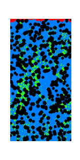
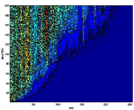
Figure 19: Top: configuration after 100 000 timesteps when flooding a water-wetting porous medium filled with water by a mixture of water and surfactant (water in blue and surfactant in green). The direction of the invasion is from left to right. Bottom: normalised concentration of surfactant versus time and versus the y-coordinate that is, in the direction of the flow (red and blue correspond to high and low concentration respectively). The concentration of surfactant in the invading fluid is 0.3. The lattice size is $128\times 256$. One time unit corresponds to 250 timesteps.

From the upper image in fig 19, we can clearly see that surfactant particles gather in the smallest pores, where the flow velocity is small. The lower image in the same figure represents the coloured concentration profile of surfactant versus time and versus the lattice row number (i.e. in the flow direction). This quantity is averaged over all columns of the lattice. The start of the simulation corresponds to the bottom line on this diagram, at which point there is no surfactant present. The appearance of a new colour (light blue) corresponds to the advance of the front of surfactant (represented approximately by the diagonal “front” in this image). We can see that the progression of the surfactant front does not exactly follow a constant speed. Indeed, zones of high surfactant concentration appear (represented by red peaks); these correspond to the formation of micelles. We can see that the micelles are stable in time, both from the point of view of their concentration (which actually even shows a tendency to increase) and of their localisation (the surfactant density peaks are vertical, indicating that the micelles do not move). The advance of surfactant is thus held up by the micellisation process; the water advances faster than the surfactant.

Structure

Here the structural properties of the front during imbibition simulations are investigated. During an invasion simulation, the precise location of the interface can be extracted. Only sites at the water-oil or surfactant-oil interface are taken into account (the obstacle sites are discarded). From these data, the fractal dimension of the interface can be calculated. This is achieved by counting the number of boxes needed to cover the interface for different box sizes. The fractal dimension is the slope of the linear part, in a log-log diagram, of the evolution of the number of boxes versus the size of the box (the so-called box counting method). At the beginning of the simulation, the interface is flat, and so the fractal dimension is equal to $1$. As invasion takes place, the interface becomes more complex and the resulting fractal dimension increases to reach a maximum value at the water percolation threshold. Simulations have been performed in order to compare the fractal dimension of the front in the binary and ternary cases. Figure 20 - bottom shows the results obtained from several of these simulations. It can be seen that the difference between the two curves (binary and ternary case) is very small, implying that the fractal dimension of the front is the same in both cases. The fractal dimension of the porous medium (equal to $1.65$), also shown in figure 20 - bottom, is greater than that associated with the invading fronts. One might thus wonder if the fractal dimension of the front is not substantially controlled by the complexity of the porous medium. Indeed, the linear part of these curves appears at scales larger than $10$ lattice sites, which is greater than the average pore size (here equal to $8.4$). The shape of the front during invasion could be imposed by the porous medium. Simulations of invasion in the absence of porous medium help to resolve this issue. Simulations with different surfactant concentrations have been run, and the results are displayed figure 20 - top.

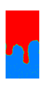
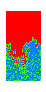
Figure 20: Top: configurations during invasion without porous medium, for concentration of surfactant of $0.1$ (left) and $0.3$ (right). Bottom: computation of the fractal dimension of the interface (on a log-log diagram , with a basis of 10). The lower two curves show the calculation of the associated fractal dimension in the absence of porous medium (dot-dashed line for $10\%$ surfactant, dashed line for $30\%$ surfactant). The curves in the middle ($D=1.6$) correspond to the invasion of binary (dot-dashed line) and ternary (dashed line) mixture ($\rho_{surf}=0.2$) into one water-wetting (index of wettability equal to $-7$) porous medium shown in figure 19. The upper curve (continuous line) is a calculation of the fractal dimension associated with the porous medium alone. The y-axis refers to the number of square boxes (length along the x-axis, in lattice site units) needed to cover the oil/water and oil/surfactant interfaces.

In the case of low concentration of surfactant (figure 20 - top) which leads to similar results as in the absence of surfactant, the interface exhibit two smooth bumps. On the other hand, when the concentration of surfactant is greater ($0.3$), the interface becomes much more complicated. The calculation of the fractal dimension in these two cases leads to the values $1.1$ and $1.35$ respectively (lower part of figure 20). Simulations with higher surfactant concentrations produce the same fractal dimensions as the latter case. Thus the fractal dimension of the invasion front evolves from $1.0$ or $1.1$ to $1.3$ when the proportion of surfactant changes from $0$ to $50\%$. We can see that the linear regime in these log-log plots persists down to box sizes of a few lattice sites, meaning that interfacial complexity still exists at this scale. For invasion simulations in porous media, the high values of the fractal dimensions are found at large scales, and a decrease of the slopes is observed at smaller scales, where the interfacial structure is not imposed by the porous medium but rather follows the shape described in the absence of porous medium.
Another, more intuitive, means of characterising the interface is simply to compute its length (i.e. the number of sites that it occupies). It is calculated in the same way as above by counting the number of interfacial sites (for example a blue site is at the interface if one of its neighbours is not a blue site nor an obstacle site). Results are displayed in figure 21.

Figure 21: Length of the oil-water interface in the binary case (dotted line) and in the ternary case ($\rho_{surf}=0.2$)(continuous line), calculated during invasion into a porous medium (the same as in fig 19, with a wettability index = -7). The vertical axis measures the number of lattice sites occupied by the interface and the horizontal axis shows the timestep in the simulation. The lattice size is $128\times 256$.

In both binary and ternary invasion, at the beginning of the simulation, the interfacial length grows. This growth is approximately the same in the two cases, and is roughly linear with time over the first 20000 timesteps. No obvious reasons are apparent for this linear time evolution. The point at which linear growth halts corresponds approximately to the onset of water percolation. In the binary case, after the linear regime, the length of the interface begins to decrease. This is related to the fact that oil droplets do not break into smaller droplets but rather escape from the lattice, leading to a reduction of the interfacial length. On the other hand, in the ternary case, beyond the linear regime, the surfactant particles induce the breaking of large oil droplets into smaller ones, thus increasing the overall length of the interface, even though the total number of oil particles decreases as invasion drives them from the lattice. This is due to emulsification, and to the fact that the structure of the interface in the ternary case is much more complex.

Timescale of micelle and emuslification phenomena

In this part, we discuss the time scale of the phenomena described above, due to the introduction of surfactant.
First of all, the formation of a complex interface appears quickly after the beginning of the simulation, well before the onset of water percolation. The phenomena of micellisation and emulsification are coupled together and appear on the same time scale. Figure 22 shows the results obtained when invading a porous medium filled with oil with a mixture of surfactant and water or simply by water. Three simulations have been run in each case. The forcing level is very small (equal to $0.001$).

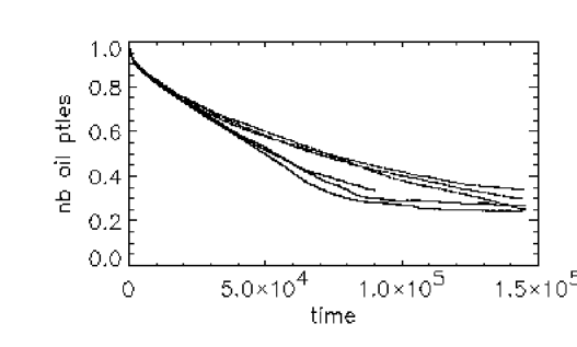
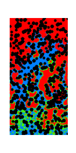
Figure 22: Left: time evolution of the number of oil particles when invading an oil-filled water-wetting porous medium with water (three continuous lines) or with a mixture of water and surfactant ($\rho_{surf}=0.2$)(three upper dotted lines). The three curves in each case correspond to three independent similar simulations. The forcing level is $0.001$. Right: a snapshot of the case with surfactant after $70000$ timesteps.

We can see that the curves associated with invasion without surfactant lie below the curves associated with the surfactant case. This means that the invasion of pure water is faster. The main differences in the curves appear near water percolation ($\sim 80000$ timesteps). After this point, the curves corresponding to the surfactant containing fluid continue to decrease while those associated with pure water invasion become flat. This suggests that in the case of pure water invasion, the oil percolation state is ended while in the case with surfactant, particles of oil continue to flow within the medium. We expect that the asymptotic value, that is residual oil saturation, will be smaller in the surfactant case, due to the flow of small oil droplets.
The slowing-down of the invasion process when surfactant is present can be understood qualitatively in terms of “gel” formation. In the snapshot image in figure 22, we can see a large number of micelles and/or small oil droplets surrounded by surfactant accumulating at the bottom of the lattice from where invasion takes place. This accumulation of micelles prevents the invading fluid from passing through, slowing down the invasion process. This is analogous to the known formation of gel by accumulation of surfactant or polymer in actual flooding experiments or reservoir treatments. Over long times, the effect of surfactant is to enhance oil recovery, as can we expect from figure 22.
Some additional simulations at higher forcing levels have been run, with the same initial conditions: the results are shown figure 23.

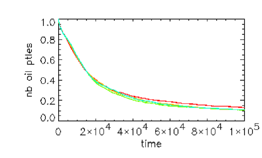
Figure 23: Temporal evolution of the number of oil particles when invading an oil-filled porous medium (the same as previously used) with water (lower curves) or with a mixture of water and surfactant ($\rho_{surf}=0.2$)(upper curves). The forcing level is $0.005$ and the lattice size is $128\times 256$. Two similar independant simulations heve been performed in each case.

Two simulations have been run in each case (with and without surfactant). The results with and without surfactant present in the invading phase fluid are identical, implying that a gel-like phase does not exist anymore; its structure is destroyed by the greater flow rates used here.
In conclusion, the formation of a gel-like phase is observed at low forcing levels, when the invasion process is slow. Its formation is due to the self assembly of micelles in pores. The effect of surfactant when the forcing level is high is small and, in some cases negligible. From these simulations, we conclude that surfactant fluids need a significant period of time to produce new features through self-assembly processes. Their action involves the formation of micelles and/or emulsification which can then enhance oil production during the imbibition process. However, to achieve this even at low forcing levels requires the use of high concentrations of surfactant ($\sim 30\%$), i.e. concentrations which would lead to microemulsion states under equilibrium conditions.

6 Drainage simulations

The term “drainage” is used to describe the invasion of a porous medium filled with wetting fluid by a non-wetting one. Simulations are performed in an oil-wetting porous medium displayed in figure 25. The lattice size is $128\times 256$. The effect of the applied force and the presence of surfactant in the invading phase are described.

6.1 Effect of applied force

The methodology is the same as in our imbibition simulations (section 5) apart from the fact that the medium is oil-wetting. Simulations are performed with a wettability index of $+7$, for different fluid forcing levels. Results are displayed in figure 24, for the binary immiscible case.

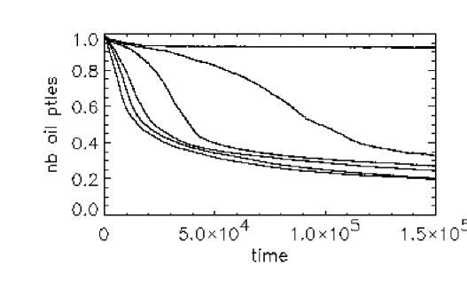
Figure 24: Temporal evolution of the number of oil particles remaining on the $128\times 256$ lattice when invading an oil-filled oil-wetting porous medium with water. The various curves are at forcing levels $0.005$, $0.01$, $0.02$, $0.03$, $0.04$, and $0.05$, from top to bottom.

At very low forcing levels (upper curve), the non-wetting fluid cannot enter the medium because of the capillary forces: the applied force on the non-wetting fluid has to exceed the capillary force to allow invasion. For greater driving forces, the speed of the invasion process is roughly proportional to the applied force. As in the case of imbibition, a maximum flow speed is reached at high forcing levels. The residual oil saturation decreases when the applied force increased, as previously observed in our imbibition simulations.
Three regimes can be distinguished during the invasion process: first, the non-wetting fluid invades the medium, displacing the wetting fluid. Secondly, the non-wetting fluid percolates, but the still flowing wetting fluid retains its connectivity to the top of the lattice. The last regime corresponds to flow of the non-wetting fluid through a medium containing stagnant residual wetting fluid.

6.2 Effect of surfactant

The effect of the presence of surfactant in the invading fluid is now investigated. Simulations have been performed with a $+7$ wettability index (i.e. strongly oil-wetting), a driving force of $0.02$ using the gravity condition, a reduced density of $0.5$ and for concentrations of surfactant equal to $0$, $15\%$, and $30\%$. Results are displayed in figure 25.

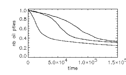
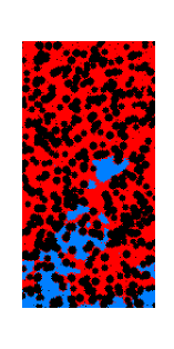
Figure 25: Left: temporal evolution of the number of oil particles remaining on a $128\times 256$ lattice when invading an oil filled oil-wetting porous medium with water (lower curve) or with a mixture of water and surfactant ($15\%$ surfactant in the invading fluid (intermediate curve) and $30\%$ (upper curve)). The forcing level is $0.02$. Right: a snapshot of the simulation during the binary fluid invasion process (oil in red and water in blue).

We can see that the temporal evolution of the number of oil particles changes dramatically when surfactant is added to the invading fluid. Going from $0$ to $30\%$ surfactant concentration, the speed (or the efficiency) of the displacement process is slowed down by more than a factor of $2$. The residual oil saturation appears to be lower ($\sim 5-10\%$) in the case of pure water invasion.
Figure 26 displays the oil concentration profile for drainage simulations with and without surfactant.

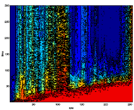
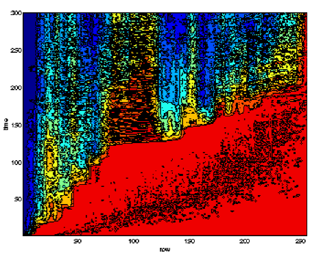
Figure 26: Normalised coloured oil concentration profile (red and blue correspond to high and low concentration respectively) versus time and y-coordinate (direction of the flow) in the case of drainage without (top) and with surfactant (bottom)(at $30\%$ concentration) present in the invading phase. The porous medium is shown in figure 25. One time unit corresponds to 250 timesteps.

The red region is greater in the case with surfactant, showing that the process is slower. Moreover, we can see that the progression of water follows a stepwise increase. This feature is more marked in the case with surfactant (lower part of figure 26). It is due to the fact that the non-wetting fluid experiences a delay before it is able to enter a channel. Visual inspection reveals that the invading fluid does not take the same path when surfactant is present as when it is absent. In the surfactant case, the path is much more tortuous. In experiments, there is some indirect evidence that paths can be different, depending on the nature of the invading fluid [19]. Our numerical results appear to confirm this behaviour.

7 Conclusion

A two-dimensional hydrodynamic lattice gas model has been used to study the behaviour of complex multiphase and amphiphilic fluids under various conditions in two dimensions. In simple cases, the results from this model agree well with theoretical predictions. In more complex geometries like porous media (where theoretical predictions in general cannot be made), an extension of Darcy’s law has been used, which explicitly admits a viscous coupling between the fluids. This coupling appears to be non-negligible, and exhibits a maximum for a 1:1 water and oil mixture. Such strong viscous coupling may be understood in terms of the spatial dimensionality of the model. The introduction of surfactant does not change the response of oil and water dramatically but it lowers the capillary threshold. On the other hand, during imbibition, introduction of surfactant leads to the appearance of new and complex features, including emulsification and micellisation. At very low fluid forcing levels, this leads to the production of a low-resistance gel, which then slows down the progress of the invading fluid. At long times (beyond the water percolation threshold), the concentration of remaining oil within the porous medium is lowered by the action of surfactant, thus enhancing oil recovery. The converse behaviour is observed in drainage simulations: the introduction of surfactant leads to a reduction in the invasion process and an increase in the residual oil saturation. Similar studies are now underway using a three dimensional version of our amphiphilic lattice gas [6].

8 Acknowledgments

Fruitful discussions with Bruce Boghosian, James Wilson, Phillip Fowler and Omar Al-Mushadani are gratefully acknowledged. We are grateful to Keir Novik for his assistance in converting colour images to the greyscale versions included here.

9 Appendix: Temporal versus ensemble averaging

In most of the simulations presented in this paper, averaging of the fluctuations inherent in our lattice gas model has been performed over time, when a steady state has been reached, rather than over an ensemble of different simulations. When using fully periodic boundary conditions, all simulations were started from an initially random configuration, independent initial configurations being constructed using different seeds for the random number generators. Assuming the existence of a steady state, and the ergodicity of the system, we can use the ergodic theorem to argue that averaging in time is equivalent to ensemble averaging. Tests have been made concerning the equivalence of these two procedures, and they show that the difference between temporal and ensemble averaging is small (roughly $\sim 2.0\%$ for medium forcing levels, although this increases when the forcing becomes very small).
The results obtained in this paper can thus be compared to those obtained using an ensemble-averaging procedure.
However, some thought reveals that ensemble-averaging may not always lead to reliable results. For example, consider a simulation using fully periodic boundary conditions, with a mixture of $10\%$ oil and $90\%$ water in a water-wetting porous medium, forcing only water, the simulation starting from an initially random configuration. The oil particles coalesce and form a droplet which flows. Now consider a simulation starting from a special condition, that is a large oil bubble trapped in the same porous medium; the probability to get such an unusual configuration from a random initial distribution is negligible (it is essentially of zero measure). The calculated oil flux for the bubble, whose stable position can be found from a preliminary imbibition simulation, will be zero. Which simulation produces the more relevant results ? From the point of view of the experiments, if the medium is at its residual oil saturation, the flow of water will not induce a flow of oil and thus the appropriate simulation is the one starting with a chosen special initial configuration; but this has a negligible probability of being sampled in a conventional ensemble-average. The problem with applying ensemble-averaging to invasion simulations is that these systems are not ergodic in general; nor indeed are their steady states equilibrium states. It is therefore a more reliable strategy to perform and report averages based on temporal behaviours in steady-states, as has generally been done in this paper.

References

- [1] U. Frisch, B. Hasslacher and Y. Pomeau (1986). Lattice-Gas Automata for the Navier-Stokes Equation. Physical Review Letters, .
- [2] S. Wolfram (1986). J. Stat. Phys., .
- [3] D. H. Rothman and J. M. Keller (1988). Immiscible Cellular-Automaton Fluids. J. Stat. Phys., .
- [4] B. M. Boghosian, P. V. Coveney and A. N. Emerton (1996). A lattice-gas model of microemulsions. Proc. R. Soc. Lond. A, .
- [5] B. M. Boghosian, P. V. Coveney and P. J. Love (1999). Three dimensional hydrodynamic lattice gas model for amphiphilic fluid dynamics. Proc. R. Soc. Lond. A, in press.
- [6] J.-B. Maillet P. J. Love and P. V. Coveney (1999). Three dimensional hydrodynamic lattice gas simulations of binary immiscible and ternary amphiphilic fluid flow through porous media, in preparation.
- [7] J. L. Wilson and P. V. Coveney (1997). Schlumberger internal scientific report. SCR/SR/1997/038/FCP/U.
- [8] L. P. Kadanoff, G. R. McNamara and G. Zanetti (1987). A poiseuille viscometer for lattice gas automata. Complex systems, .
- [9] P. V. Coveney, J.-B. Maillet, J. L. Wilson, P. W. Fowler, O. Al-Mushadani and B. M. Boghosian (1998). Lattice gas simulations of ternary amphiphilic fluid flow in porous media. Inter. Journal of Modern Physics C, .
- [10] D. H. Rothman and S. Zaleski. Lattice-gas cellular automata. (1997). Cambridge University Press.
- [11] D. H. Rothman (1990). Macroscopic laws for immiscible two-phase flow in porous media: results from numerical simulations. Journal of Geophysical Research, .
- [12] F. Kalaydjian (1990). Origin and quantification of coupling between relative permeabilities for two-phase flows in porous media. Transport in porous media, .
- [13] J. F. Olson and D. H. Rothman (1997). Two-fluid flow in sedimentary rock: simulation, transport and complexity. J. Fluid. Mech, .
- [14] C. Zarcone and R. Lenormand (1994). Détermination expérimentale du couplage visqueux dans les écoulements diphasiques en milieux poreux. C. R. Acad. Sci. Paris, .
- [15] P. A. Goode and T. S. Ramakrishnan (1993). Momentum transfer across fluid-fluid interfaces in porous media: a network model. AIChE Journal, .
- [16] P. Fowler and P. V. Coveney (1998). Unpublished work.
- [17] J.-B. Maillet, V. Lachet and P. V. Coveney (1999). Large scale molecular dynamics simulation of self-assembly processes in short and long chain cationic surfactant. Phys. Chem. Chem. Phys., in press.
- [18] P. V. Coveney, A. N. Emerton and B. M. Boghosian (1996). Simulation of self-reproducind micelles using a lattice-gas automaton. J. Am. Chem. Soc., .
- [19] P. Tardy and S. Olthoff, private communication.