Dynamics of Br Electrosorption on Single-Crystal Ag(100): A Computational Study

Abstract

We present dynamic Monte Carlo simulations of a lattice-gas model for bromine electrodeposition on single-crystal silver (100). This system undergoes a continuous phase transition between a disordered phase at low electrode potentials and a commensurate c($2\times 2$) phase at high potentials. The lattice-gas parameters are determined by fitting simulated equilibrium adsorption isotherms to chronocoulometric data, and free-energy barriers for adsorption/desorption and lateral diffusion are estimated from ab initio data in the literature. Cyclic voltammograms in the quasi-static limit are obtained by equilibrium Monte Carlo simulations, while for nonzero potential scan rates we use dynamic Monte Carlo simulation. The butterfly shapes of the simulated voltammograms are in good agreement with experiments. Simulated potential-step experiments give results for the time evolution of the Br coverage, as well as the c($2\times 2$) order parameter and its correlation length. During phase ordering following a positive potential step, the system obeys dynamic scaling. The disordering following a negative potential step is well described by random desorption with diffusion. Both ordering and disordering processes are strongly influenced by the ratio of the time scales for desorption and diffusion. Our results should be testable by experiments, in particular cyclic voltammetry and surface X-ray scattering.

Keywords: Bromine adsorption; Continuous phase transition; Cyclic Voltammetry; Dynamic Monte Carlo simulation; Lattice-gas model; Potential-step experiments;

1 Introduction

The electrodeposition of Br on single-crystal Ag(100) from aqueous solution is a simple example of anion adsorption which has been extensively studied, both by classical electrochemical methods [1, 2, 3, 4, 5] and by techniques such as in situ surface X-ray scattering (SXS) [2, 3, 4] and X-ray absorption fine structure (XAFS) [5].

Cyclic voltammetry (CV) shows a typical butterfly structure with a broad pre-wave in the negative-potential region and a sharp peak at more positive potentials [1, 2, 3, 4, 5]. The recent SXS experiments by Ocko, Wang, and Wandlowski [2] showed that the sharp peak corresponds to a continuous phase transition in the layer of adsorbed Br. At this transition the adlayer changes its structure from a disordered two-dimensional “gas” on the negative-potential side, to an ordered, commensurate c($2\times 2$) phase with a Br coverage of 1/2 monolayer on the positive side. The pre-wave lies wholly in the disordered-phase region, and it was previously suggested that it was caused by interactions with surface water [1]. However, equilibrium Monte Carlo (MC) simulations of water-free lattice-gas models of the Br adlayer by Koper [6, 7], as well as our own work reported here, produce quasi-equilibrium cyclic voltammograms (CVs) of essentially the same shape as the experiments, indicating that surface water is not needed to reproduce the pre-wave. Rather, we believe that the pre-wave is due to short-range correlations in the disordered adlayer [6, 8]. In this system, the structures that give rise to these correlations locally resemble low-temperature ordered phases with coverage 1/4.

The simplicity of the equilibrium properties of this system makes it a prime candidate for dynamic studies. Here we present results from such a study by dynamic MC simulation [9] of a lattice-gas model. This method has the advantage over mean-field rate-equation approaches that it properly accounts for the effects of local fluctuations in the adlayer structure. Further details and additional results will be presented elsewhere [10]. Animations and additional figures are available on the World Wide Web [11].

The rest of this paper is organized as follows. The lattice-gas model is presented in Sec. 2, followed by equilibrium simulations which are used to estimate the lattice-gas model parameters by fitting to adsorption isotherms from chronocoulometry experiments [2, 3, 4]. In Sec. 3 we present simulated CVs (Sec. 3.1) and potential-step experiments (Sec. 3.2). From the the potential-step simulations we provide current transients, which are easy to measure in electrochemical experiments, as well as predictions for the time evolution of the intensity of the SXS scattering peak corresponding to the c($2\times 2$) phase. Although dynamic SXS data have yet to be obtained for this system, they were obtained for others [12], and we believe it is only a matter of time before such experimental results become available.

2 Model and Equilibrium Results

We use a lattice-gas model similar to the one used by Koper [6]. It consists of an $L\times L$ square array of Br adsorption sites, corresponding to the four-fold hollow sites on the Ag(100) surface. The configurational energy of the Br adlayer is given by the grand-canonical lattice-gas Hamiltonian,

$${\cal H}=-\sum_{i<j}\phi_{ij}c_{i}c_{j}-\overline{\mu}\sum_{i=1}^{L^{2}}c_{i}\;.$$ (1)

Here $i$ and $j$ denote adsorption sites, $c_{i}$ is the occupation at site $i$, which is either 0 (empty) or 1 (occupied), $\sum_{i<j}$ is a sum over all pairs of sites, $\phi_{ij}$ is the lateral interaction energy of the pair $(i,j)$, and $\overline{\mu}$ is the electrochemical potential. The sign conventions are such that $\phi_{ij}<0$ denotes a repulsive interaction, and $\overline{\mu}>0$ favors adsorption. We measure $\phi_{ij}$ and $\overline{\mu}$ in units of meV/pair and meV/particle, respectively. (For brevity, both will be written simply as meV.) To reduce finite-size effects, we use periodic boundary conditions.

In the weak-solution approximation, $\overline{\mu}$ is related to the electrode potential by

$$\overline{\mu}=\overline{\mu}_{0}+k_{\rm B}T\ln\frac{[C]}{[C_{0}]}-e\gamma E\;,$$ (2)

where $\overline{\mu}_{0}$ is an arbitrary reference level, $k_{\rm B}$ is Boltzmann’s constant, $T$ is the absolute temperature, $e$ is the elementary charge unit, $[C]$ is the concentration of Br^- in solution, $[C_{0}]$ is an arbitrary reference concentration, $\gamma$ is the electrosorption valency, and $E$ is the electrode potential in mV.

Previously Koper has explored the effects of finite nearest-neighbor repulsion and screened dipole-dipole interactions in this model [6]. As his results indicate only minor effects of the finite nearest-neighbor repulsion and screening, we here use a simplified model with nearest-neighbor exclusion and unscreened dipole-dipole interactions. Thus, the long-range part of the interaction energy is $\phi(r)={2^{3/2}\phi_{\rm nnn}}{r^{-3}}$ for $r\geq\sqrt{2}$, where $r$ is the separation of an interacting Br pair, measured in units of the Ag(100) lattice spacing ($a=2.889$ Å [2]), and $\phi_{\rm nnn}$ (which is negative) is the lateral dipole-dipole repulsion between next-nearest neighbors. For computational convenience we cut off the long-range interaction for $r>5$. This underestimates the total interaction energy of a fully occupied c($2\times 2$) layer by about $13\%$.

The nearest-neighbor exclusions give rise to two different sublattices of possible adsorption sites (like the black and white squares on a chessboard). Each sublattice (labeled $A$ and $B$, respectively) corresponds to one of two degenerate c$(2\times 2)$ phases. The $A$ sublattice coverage is the fraction of occupied sites on sublattice $A$, defined as $\Theta_{A}=N_{A}^{-1}\sum_{i\in A}^{N_{A}}c_{i}$, where $N_{A}$ is the number of sites on sublattice $A$ and $\sum_{i\in A}^{N_{A}}$ runs over all sites on the sublattice. We define $\Theta_{B}$ analogously.

The sublattice coverages combine to give two observables of interest: the total Br coverage $\Theta=(\Theta_{A}+\Theta_{B})/2$, and the “staggered” coverage $\Theta_{\rm S}=\Theta_{A}-\Theta_{B}$, which is the order parameter for the c$(2\times 2)$ phase. While $\Theta$ can be experimentally obtained by standard electrochemical methods, as well as from the integer-order peaks in scattering data, $\Theta_{\rm S}$ is proportional to the square root of the intensity in the half-order diffraction peaks that correspond to the c$(2\times 2)$ phase [2].

To estimate the parameters in the lattice-gas model, $\phi_{\rm nnn}$ and $\gamma$, we performed standard equilibrium MC simulations [13] at room temperature ($k_{\rm B}T=25$ meV or $T\approx 290$ K) to obtain $\Theta(\overline{\mu})$ for different parameter values. These simulated isotherms were then compared with experimental chronocoulometry data for three different electrolyte concentrations [3, 4], and the best parameter values were determined by a nonlinear fit [10]. The resulting values are $\phi_{\rm nnn}=-26\pm 2$ meV and $\gamma=-0.73\pm 0.03$. These results are consistent with those found previously [3, 4, 6]. The fitted MC isotherm is shown together with the experimental isotherms in Fig. 1. Especially for the two lowest concentrations, the agreement is excellent over the whole range of electrode potentials. The kinks in the isotherms, observed at $\Theta_{c}\approx 0.37$ for both the experiments and simulations, correspond to the order–disorder phase transition. To within our statistical uncertainty, this value of $\Theta_{c}$ is consistent with previous results for a square-lattice model with only nearest-neighbor exclusion, known as the “hard-square model” [14, 15, 16].

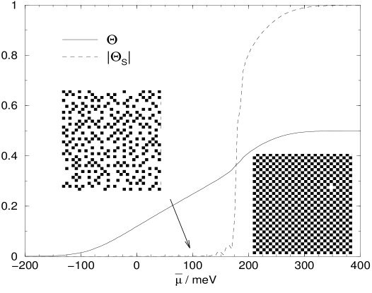
Figure 2: Equilibrium Monte Carlo isotherms for $L=32$, $T\approx 290$ K, and $\phi_{\rm nnn}=-26$ meV. A continuous phase transition between a low-coverage disordered phase and a c$(2\times 2)$ phase with $\Theta=1/2$ occurs at $\bar{\mu}_{c}\approx 180$ meV. The order parameter for the c$(2\times 2)$ phase is $|\Theta_{\rm S}|$. These isotherms are obtained from 10,000 independent samples for each value of $\bar{\mu}$. The insets show typical equilibrium configurations in the disordered phase at $\bar{\mu}=+100$ meV (left) and in the ordered phase at +400 meV (right).

The simulation data for $\Theta(\bar{\mu})$ and $\Theta_{\rm S}(\bar{\mu})$ with the best-fit interaction parameter $\phi_{\rm nnn}=-26$ meV are shown together in Fig. 2. As $\bar{\mu}$ approaches its critical value at $\bar{\mu}_{c}=180\pm 5$ meV from the positive side, $\Theta_{\rm S}\propto(\bar{\mu}-\bar{\mu}_{c})^{1/8}$. This behavior of the order parameter is consistent with the Ising universality class, to which this system belongs, and was confirmed by SXS experiments [2]. Typical equilibrium configurations are shown as insets in Fig. 2 for the disordered phase at $\bar{\mu}=+100$ meV and for the ordered phase at $\bar{\mu}=+400$ meV.

A simulated quasi-equilibrium CV, corresponding to a vanishing potential-sweep rate, can be obtained from the MC equilibrium isotherm as

$${\cal J}=-\gamma eM\frac{d\Theta}{dt}=-\gamma eM\frac{d\Theta}{d\bar{\mu}}\frac{d\bar{\mu}}{dE}\frac{dE}{dt}=\gamma^{2}e^{2}M\frac{d\Theta}{d\bar{\mu}}\frac{dE}{dt}\propto\frac{d\Theta}{d\bar{\mu}}\;,$$ (3)

where ${\cal J}$ is the voltammetric current density (oxidation currents positive), $M$ is the total number of adsorption sites per unit area ($a^{-2}=1.198\times 10^{15}$ sites/cm²), and ${dE}/{dt}$ is the sweep rate. This limiting CV is shown in Figure 3(a) together with CVs for nonzero sweep rates, which are obtained by dynamic MC simulations discussed in Sec. 3.1. It exhibits the same broad pre-wave and sharp peak seen in experiments [1, 2, 3, 4, 5]. The broad prewave in the simulated CV is caused by configurational fluctuations in the disordered phase, which locally resemble low-temperature ordered phases [17, 18], in particular p($2\times 2$) and c($4\times 2$) with $\Theta=1/4$ [10]. Such fluctuations of local short-range order in the disordered phase are clearly seen in the inset in Fig. 2 for $\bar{\mu}=+100$meV, and they lead to visible anisotropy in simulated diffuse SXS scattering intensities [10]. This anisotropy should be experimentally observable as well.

3 Dynamic Simulations

The dynamics of the Br adsorption and desorption processes under CV and potential-step conditions were simulated with a dynamic MC algorithm including adsorption and desorption events, as well as nearest- and next-nearest-neighbor lateral diffusion of the adsorbed Br. Bulk diffusion in the solution is neglected, corresponding to a well-stirred system. Each such single microscopic move, which we label by the index $\lambda$, connects an initial lattice-gas state, $I$, to a final state, $F$. The energies of these states, $U_{I}$ and $U_{F}$, are obtained by applying the lattice-gas Hamiltonian, Eq. (1), to the corresponding configurations. An intermediate transition state of higher energy, $T_{\lambda}$, is associated with the move $\lambda$. This intermediate state cannot be represented by a lattice-gas configuration, and we associate with it a “bare” free-energy barrier, $\Delta_{\lambda}$. Using a symmetric Butler-Volmer approximation [9, 10, 19], we can then approximate the free energy of the transition state as

$$U_{T_{\lambda}}=\frac{U_{I}+U_{F}}{2}+\Delta_{\lambda}\;.$$ (4)

Although other choices of the transition probability are also found in the literature [20], we here approximate the probability $R(F|I)$ of making a transition from $I$ to $F$ during a single MC time step by the one-step Arrhenius rate [9, 21, 22]

$$R(F|I)=\nu\exp{\left(-\frac{U_{T_{\lambda}}-U_{I}}{k_{\rm B}T}\right)}=\nu\exp{\left(-\frac{\Delta_{\lambda}}{k_{\rm B}T}\right)}\exp{\left(-\frac{U_{F}-U_{I}}{2k_{\rm B}T}\right)}\;,$$ (5)

where the dimensionless rate constant $\nu$ relates the simulation time scale, measured in MC steps per site (MCSS), to the experimental time scale in seconds. In our simulations we used $\nu=1$.

We performed the simulation with a simple discrete-time dynamical algorithm, in which new configurations are randomly chosen from a weighted list of microscopic moves. First, a particular lattice site is chosen at random. The configuration can then be changed only through moves which include the chosen site. If the site is empty, adsorption is attempted and accepted with probability given by Eq. (5). If any of the nearest-neighbor sites are occupied, this acceptance probability is zero. If the chosen site is occupied, only desorption or lateral diffusion may be attempted. A list is kept of all the possible moves, and one of them is chosen according to the corresponding acceptance probabilities. The probability to remain in the initial state is $R(I|I)=1-\sum_{F\neq I}R(F|I)$. Further details on the simulation algorithm and its implementation are given elsewhere [9, 10].

While this algorithm is of limited accuracy for very fast processes and requires an unnecessarily large amount of computer time for very slow processes [21, 23, 24, 25, 26, 27], it has the advantages that it is easy to program and is readily adapted to simulations in which parameters (such as $\bar{\mu}$) change with time [27]. It is thus well suited for dynamic CV simulations.

The free-energy barriers associated with the different simulation moves are $\Delta_{\rm nn}$ for nearest-neighbor diffusion, $\Delta_{\rm nnn}$ for next-nearest neighbor diffusion, and $\Delta_{\rm a}$ for adsorption/desorption. The rough estimates used here, $\Delta_{\rm nn}=100$ meV and $\Delta_{\rm nnn}=200$ meV, are based on ab-initio calculations of binding energies for a single Br ion on a Ag(100) substrate in vacuum [28]. The difference in binding energy between the bridge site and the four-fold hollow site gives $\Delta_{\rm nn}$, and the difference between the on-top site and the four-fold hollow site gives $\Delta_{\rm nnn}$. Theoretical estimates of $\Delta_{\rm a}$ are extremely sensitive to the ion-surface and ion-water interactions [29]. Calculated potentials of mean force for halide ions in water near a Cu(100) surface [29] indicate that values between 200 and 500 meV are not unreasonable. To optimize the simulation speed, we chose $\Delta_{\rm a}=300$ meV. This value is as low as possible while remaining consistent with our expectation that it should be significantly larger than $\Delta_{\rm nnn}$.

3.1 Simulated Cyclic Voltammograms

CV experiments were simulated on systems with $L=256$ and 128 by first equilibrating at $\bar{\mu}=-400$ meV and then ramping $\bar{\mu}$ linearly in time up to +600 meV, and back down to $-$400 meV. Simulated CV currents for sweep rates between 3$\times$10^-4 and 3$\times$10^-3 meV/MCSS, divided by the sweep rate in order to be easily compared on the same scale, are shown in Fig. 3(a). The limiting curve for vanishing sweep rate is given by the quasi-equilibrium CV, obtained from the equilibrium simulations described in Sec. 2. A considerable asymmetry in the peak shape for the positive-going and negative-going scans is notable.

While the pre-waves are relatively little affected by the sweep rate, the peak corresponding to the phase transition is significantly lowered and shifted in the scan direction. The dependence of the peak separation on the sweep rate, which is a form of hysteresis [30], is shown in Fig. 3(b).

By comparing the scan-rate dependence of the separation between the positive-going and negative-going peak positions in simulations and experiments, one can in principle obtain a rough estimate of the relation between simulation time and physical time, provided the free-energy barriers used in the simulations are in a reasonably realistic proportion to each other. The peak separations observed in our simulations, Fig. 3(b), are large compared to typical experimental values of a few tens of meV for scan rates in the range 1-10 mV/s. This most likely indicates that even our slowest simulated scan rates correspond to faster scans in the real system. Direct comparisons between simulation and experimental dynamic effects are left for future research.

3.2 Simulated Potential Steps

Dynamic potential-step simulations were performed on systems with $L=256$. They began by equilibrating the system at room temperature and potential $\bar{\mu}_{1}$. After equilibration, $\bar{\mu}$ was instantaneously stepped to a new value, $\bar{\mu}_{2}$, and the simulation was continued by the dynamic MC algorithm described above. To illustrate the dynamics of the phase ordering and disordering processes, we here show results for two different potential steps: one from the disordered phase into the ordered phase, and one from the ordered phase into the disordered phase. Additional potential-step simulations and corresponding time-dependent SXS scattering intensities will be reported elsewhere [10].

3.2.1 Disorder-to-order step

For the disorder-to-order step we used $\bar{\mu}_{1}=-200$ meV and $\bar{\mu}_{2}=+600$ meV. At $\bar{\mu}_{1}$ the coverage is close to zero, while $\bar{\mu}_{2}$ is far into the ordered phase, approximately $420$ meV past the phase transition at $\bar{\mu}_{c}$. In Fig. 4 we show both $\Theta$ and $\Theta_{\rm S}$ vs time. With deep steps like this one, the desorption rate is negligible. Thus, the adsorption dynamics are essentially described by the random sequential adsorption with diffusion (RSAD) process [31, 32]. The coverage quickly reaches the jamming coverage for random sequential adsorption of hard squares without diffusion, $\Theta_{\rm J}=0.364$ [33, 34] (only slightly below the critical coverage, $\Theta_{c}\approx 0.37$). At this coverage both sublattices contain small, uncorrelated domains of the two degenerate ordered phases, separated by domain walls. The domain walls consist of empty sites, most of which cannot be filled, due to the nearest-neighbor exclusion.

At later times, the coverage can increase only where domain walls move together, opening a gap large enough to fit an additional Br. The domain-wall motion responsible for opening additional adsorption sites proceeds almost exclusively through nearest-neighbor diffusion between adjacent domains. The coverage approaches the equilibrium value, $\Theta_{\rm eq}=1/2$, and the total length of interfaces decreases. The order-parameter correlation length, $D$, is experimentally measurable as the inverse width of the half-order diffuse SXS scattering maxima [2, 12]. Since $D$ is also proportional to the inverse of the interfacial length per unit area [35], it can in the present case be estimated from the coverage as $D=(\Theta_{\rm eq}-\Theta)^{-1}$ [31, 32]. The dynamic scaling theory of the kinetics of phase transitions predicts that, for systems with nonconserved order parameter (such as the one considered here) undergoing phase ordering, $D$ should grow with time as $t^{1/2}$ [36]. The inset in Fig. 4 shows $D$ as a function of $t^{1/2}$. The agreement with the expected dynamic scaling behavior is excellent, as has also been found in previous simulations of RSAD [31, 32].

For an infinite system, $D$ would continue to grow without bound; however, when $D$ reaches the same order of magnitude as $L$, the system enters the phase-selection regime in which one of the two degenerate ordered phases grows to fill the whole system. Our step simulations were too short to study the phase-selection regime in detail. Results for shallower positive-going potential steps, which are somewhat less clear-cut than for the deep step shown here, will be reported elsewhere [10].

3.2.2 Order-to-disorder step

For deep order-to-disorder steps, the disordering process is rather simple. Particles desorb at a roughly constant rate, leading to an essentially exponential relaxation to equilibrium [10].

After a shallow order-to-disorder step, $\bar{\mu}_{1}=+600$ meV and $\bar{\mu}_{2}=+100$ meV, the behavior is more interesting. The system starts with all particles on sublattice $A$ and relaxes to a disordered phase with $\Theta\approx 1/4$, as shown in Fig. 5. There are four different dynamical regimes. In the first regime, particles simply desorb from sublattice $A$ so that $d\Theta_{\rm S}/dt\approx 2\,d\Theta/dt$. As more sites become vacant, small domains are formed on sublattice $B$ both by lateral diffusion from sublattice $A$ and by adsorption from the solution. In this second regime, both desorption and diffusion contribute significantly to the disordering process. In the third regime, the adsorption and desorption rates are almost equal and relatively slow, and diffusion is the dominant contribution to the disordering. Here $d\Theta_{\rm S}/dt$ becomes significantly larger than $d\Theta/dt$, until the two sublattices become approximately equally populated in the fourth regime, yielding $\Theta_{\rm S}\approx 0$.

4 Conclusion

In this brief paper we have presented results from dynamic MC simulations of CV and potential-step experiments for Br electrosorption on Ag(100) single-crystal electrodes. The simulations show the complicated interplay between adsorption, desorption, and lateral diffusion even in this relatively simple electrochemical system.

The dynamic MC algorithm requires estimates of free-energy barriers for adsorption/desorption and lateral diffusion. While such barrier estimates constitute the most uncertain part of a dynamic MC simulation, we were able to obtain reasonable numbers from ab initio calculations in the literature [28, 29].

As the order parameter $\Theta_{\rm S}$ and its correlation length are measurable in SXS experiments [2, 3, 4, 12], the dynamical phenomena predicted by our simulations should be observable in future experiments. Further details and simulations of time-dependent diffuse SXS scattering intensities will be reported elsewhere [10].

Figure 1: A single equilibrium Monte Carlo (MC) simulation isotherm ($L=32$, $T\approx 290$ K), fit simultaneously to coverage isotherms at three different Br^- concentrations, obtained by chronocoulometry [3, 4]. The parameters, $\phi_{\rm nnn}=-26\pm 2$ meV and $\gamma=-0.73\pm 0.03$, were obtained by a nonlinear fit to the experimental data.

Figure 3: (a) Simulated CVs for $L=128$ and 256 at various potential-sweep rates $\rho$. The curves for nonzero $\rho$ give $\rho^{-1}d\Theta/dt$, while for $\rho=0$ we show $d\Theta/d\bar{\mu}$ obtained by differentiating the simulated equilibrium coverage isotherm in Fig. 2. (b) Peak separations for various sweep rates. For experimental comparison, the units are given as mV and are obtained with $\gamma=-0.73$.

Figure 4: Coverage, $\Theta$, and order parameter, $|\Theta_{\rm S}|$, shown vs time for sudden disorder-to-order potential step at room temperature with $L$=256. Step from $\bar{\mu}_{1}=-200$ meV to $\bar{\mu}_{2}=+600$ meV, averaged over 10 independent runs. The inset shows the correlation length for the c$(2\times 2)$ order parameter vs $t^{1/2}$.

Figure 5: Coverage, $\Theta$, and order parameter, $|\Theta_{\rm S}|$, shown vs time for sudden order-to-disorder potential step at room temperature with $L$=256. The four dynamic regimes discussed in the text are labeled and separated by vertical bars. Step from $\bar{\mu}_{1}=+600$ meV to $\bar{\mu}_{2}=-200$ meV, averaged over 3 independent runs.

References

- [1] G. Valette, A. Hamelin, R. Parsons, Zeitschrift für Physikalische Chemie, Neue Folge 113 (1978) 71.
- [2] B.M. Ocko, J.X. Wang, T. Wandlowski, Phys. Rev. Lett. 79 (1997) 1511.
- [3] J.X. Wang, T. Wandlowski, B.M. Ocko, in Proceedings of the Symposium on The Electrochemical Double Layer, Electrochem. Soc. Conf. Proc. Ser. The Electrochemical Society, Pennington, NJ, (1997) Vol. 97-17, 293.
- [4] Th. Wandlowski, J.X. Wang, B.M. Ocko, submitted to J. Electroanal. Chem.
- [5] O. Endo, M. Kiguchi, T. Yokoyama, M. Ito, T. Ohta, J. Electroanal. Chem. 473 (1999) 19.
- [6] M.T.M. Koper, J. Electroanal. Chem. 450 (1998) 189.
- [7] M.T.M. Koper, Electrochim. Acta 44 (1998) 1207.
- [8] M.T.M. Koper, J.J. Lukkien, J. Electroanal. Chem., in press.
- [9] G. Brown, P.A. Rikvold, S.J. Mitchell, M.A. Novotny, in Interfacial Electrochemistry: Theory, Experiment, and Applications, A. Wieckowski (Ed.), Marcel Dekker, New York, 1999, p. 47.
- [10] S.J. Mitchell, G. Brown, P.A. Rikvold, submitted to Surf. Sci. E-print: cond-mat/0007079.
- [11] Animations and additional figures are available at http://www.csit.fsu.edu/rikvold/
- [12] A.C. Finnefrock, K.L. Ringland, J.D. Brock, L.J. Buller, H.D. Abruña, Phys. Rev. Lett. 81 (1998) 3459.
- [13] K. Binder, D.W. Heermann, Monte Carlo Simulation in Statistical Physics: An Introduction. Third edition. Springer, New York, 1997.
- [14] F.H. Ree, D.A. Chesnut, J. Chem. Phys. 45 (1966) 3983.
- [15] R.J. Baxter, I.G. Enting, S.K. Tsang, J. Stat. Phys. 22 (1980) 465.
- [16] Z. Ràcz, Phys. Rev. B 21 (1980) 4012.
- [17] P.A. Rikvold, M.R. Deakin, Surf. Sci. 249 (1991) 180.
- [18] P.A. Rikvold, Electrochim. Acta 36 (1991) 1689.
- [19] A.J. Bard, L.R. Faulkner, Electrochemical Methods: Fundamentals and Applications. Wiley, New York, 1980.
- [20] T. Ala-Nissila, J. Kjoll, S.C. Ying, Phys. Rev. B 46 (1992) 846.
- [21] H.C. Kang, W.H. Weinberg, J. Chem. Phys. 90 (1989) 2824.
- [22] C. Uebing, R. Gomer, Surf. Sci. 381 (1997) 33.
- [23] A.B. Bortz, M.H. Kalos, J.L. Lebowitz, J. Comput. Phys. 17 (1975) 10.
- [24] G.H. Gilmer, J. Crystal Growth 35 (1976) 15.
- [25] K.A. Fichthorn, W.H. Weinberg, J. Chem. Phys. 95 (1991) 1090.
- [26] M.A. Novotny, Phys. Rev. Lett. 74 (1995) 1; erratum Phys. Rev. Lett. 75 (1995) 1424.
- [27] J.J. Lukkien, J.P.L. Segers, P.A.J. Hilbers, R.J. Gelten, A.P.J. Jansen, Phys. Rev. E 58 (1998) 2598.
- [28] A. Ignaczak, J.A.N.F. Gomes, J. Electroanal. Chem. 420 (1997) 71.
- [29] A. Ignaczak, J.A.N.F. Gomes, S. Romanowski, J. Electroanal. Chem. 450 (1998) 715.
- [30] S.J. Mitchell, P.A. Rikvold, G. Brown, in Computer Simulation Studies in Condensed-Matter Physics XIII, D.P. Landau, S.P. Lewis, H.-B. Schüttler (Eds.), Springer, Heidelberg, in press. E-print: cond-mat/0006399.
- [31] J.-S. Wang, P. Nielaba, V. Privman, Mod. Phys. Lett. B 7 (1993) 189.
- [32] E. Eisenberg, A. Baram, Europhys. Lett. 44 (1998) 168.
- [33] P. Meakin, J.L. Cardy, E. Loh Jr., D.J. Scalapino, J. Chem. Phys. 86 (1987) 2380.
- [34] A. Baram, M. Fixman, J. Chem. Phys. 103 (1995) 1929.
- [35] P. Debye, H.R. Anderson, H. Brumberger, J. Appl. Phys. 28 (1957) 679.
- [36] J.D. Gunton, M. San Miguel, P.S. Sahni, in Phase Transitions and Critical Phenomena, Volume 8, C. Domb, J.L. Lebowitz (Eds.), Academic, London, 1983, p. 267.