Multi-plateau magnetization curves of one-dimensional Heisenberg ferrimagnets

Abstract

Ground-state magnetization curves of ferrimagnetic Heisenberg chains of alternating spins $S$ and $s$ are numerically investigated. Calculating several cases of $(S,s)$, we conclude that the spin-$(S,s)$ chain generally exhibits $2s$ magnetization plateaux even at the most symmetric point. In the double- or more-plateau structure, the initial plateau is generated on a classical basis, whereas the higher ones are based on a quantum mechanism.

I Introduction

Ground-state magnetization curves of low-dimensional quantum spin systems have been attracting much recent interest due to their nontrivial appearance contrasting with classical behaviors. A few years ago there appeared an epochal argument [1] in the field. Generalizing the Lieb-Schultz-Mattis theorem [2, 3], Oshikawa, Yamanaka, and Affleck proposed that magnetization plateaux of quantum spin chains should be quantized as

$$S_{\rm unit}-m=\mbox{integer}\,,$$ (1)

where $S_{\rm unit}$ is the sum of spins over all sites in the unit period and $m$ is the magnetization $M$ divided by the number of the unit cells. Their argument caused renewed interest [4] in the pioneering calculations [5, 6, 7] of a bond-trimerized spin-$\frac{1}{2}$ chain and further stimulated extensive investigations into quantum magnetization process. Quantized magnetization plateaux were reasonably detected for spin-$\frac{1}{2}$ [8], spin-$1$ [9, 10, 11], and spin-$\frac{3}{2}$ [12, 13] chains with modulated and/or anisotropic interactions. Totsuka [14], Cabra and Grynberg [15], and Honecker [16] developed calculations of general polymerized spin chains. Numerous authors have been making further theoretical explorations into extended systems including spin ladders [17, 18, 19, 20] and layered magnets [21, 22, 23]. Experimental observations [24, 25] have also followed.

Mixed-spin chains, which have vigorously been studied in recent years [26, 27, 28, 29, 30, 31, 32, 33, 34, 35, 36], also stimulate us in this context. Theoretical investigations into them are all the more interesting and important considering an accumulated chemical knowledge on ferrimagnetic materials. Kahn et al. [37] succeeded in synthesizing a series of bimetallic chain compounds such as MM^′(pba)(H₂O)₃$\cdot$$2$H₂O (pba $=$ $1,3$-propylenebis(oxamato) $=$ C₇H₆N₂O₆) and MM^′(pbaOH)(H₂O)₃ (pbaOH $=$ $2$-hydroxy-$1,3$-propylenebis(oxamato) $=$ C₇H₆N₂O₇), where the alternating magnetic ions M and M^′ are flexible variables and therefore the low-dimensional ferrimagnetic behavior could systematically be observed. Caneschi et al. [38] synthesized another series of mixed-spin chain compounds of general formula M(hfac)₂NITR, where metal ion complexes M(hfac)₂ with hfac $=$ hexafluoroacetylacetonate are bridged by nitronyl nitroxide radicals NITR. There also exist purely organic molecule-based ferrimagnets [39], where sufficiently small magnetic anisotropy, whether of exchange-coupling type or of single-ion type, is advantageous for observations of essential quantum mixed-spin phenomena.

Magnetization curves of Heisenberg ferrimagnetic chains were revealed by Kuramoto [33]. His argument covered an effect of next-nearest-neighbor interactions but the constituent spins were restricted to $1$ and $\frac{1}{2}$. Although an alignment of alternating spins $S$ and $s$ ($S>s$) in a field, as described by the Hamiltonian

$${\cal H}={\displaystyle\sum_{j=1}^{N}} \bigl{[} (1+\delta)(\mbox{\boldmath$S$}_{j}\cdot\mbox{\boldmath$s$}_{j})_{\alpha}+(1-\delta)(\mbox{\boldmath$s$}_{j}\cdot\mbox{\boldmath$S$}_{j+1})_{\alpha}$$ (2)

$$- H(S_{j}^{z}+s_{j}^{z})\bigr{]}\,,$$ (3)

with $(\mbox{\boldmath$S$}\cdot\mbox{\boldmath$s$})_{\alpha}=S^{x}s^{x}+S^{y}s^{y}+\alpha S^{z}s^{z}$, is so interesting as to possibly exhibit a series of quantized magnetization plateaux at $m=\frac{1}{2}(1),\frac{3}{2}(2),\cdots,S+s-1$, its magnetization curves have not systematically been studied so far. In spite of the vigorous argument, there are few reports on multi-plateau magnetization curves. It is true that a double-plateau structure lies in NH₄CuCl₃ [21, 25], but it is owing to the variety of exchange interactions. We here demonstrate that the ferrimagnetic chain (3) generally exhibits a $2s$-plateau magnetization curve without any anisotropy and any bond polymerization, namely, even at $\alpha=1$ and $\delta=0$. We believe that the present calculations will accelerate physical measurements on vast ferrimagnetic chain compounds lying unexploited in the field of both inorganic and organic chemistry.

The ground state of the isotropic Hamiltonian (3) without the Zeeman term, which is a multiplet of spin $(S-s)N$, exhibits elementary excitations of two distinct types [40]. The excitations of ferromagnetic aspect, reducing the ground-state magnetization, form a gapless dispersion relation, whereas those of antiferromagnetic aspect, enhancing the ground-state magnetization, are gapped from the ground state. Therefore we can readily understand the initial step at $m=S-s$ in the magnetization curve. In the Ising limit $\alpha\rightarrow\infty$, the initial plateau is nothing but the gapped excitation from the Néel-ordered state. The classical gap-generation mechanism is unique. Thus any magnetization curve in the Ising limit only has a single plateau. The scenario is qualitatively unchanged for an arbitrary $\alpha$ as long as we consider the classical vectors $\mbox{\boldmath$S$}_{j}$ and $\mbox{\boldmath$s$}_{j}$ of magnitude $S$ and $s$ instead of quantum spins. Therefore, the second and higher plateaux, if any, should generally be based on a quantum mechanism.

FIG. 1.: The ground-state magnetization curves for the Hamiltonian (2) with $\delta=0$ at various values of $\alpha$ and $(S,s)$.

FIG. 2.: (a) Schematic representations of the $M=(S-s)N$ ground states of spin-$(S,s)$ ferrimagnetic chains of $N$ elementary cells in the decoupled-dimer limit. The arrow (the bullet symbol) denotes a spin $\frac{1}{2}$ with its fixed (unfixed) projection value. The solid segment is a singlet pair. (b) A ferrimagnet may be regarded as the combination of a ferromagnet and an antiferromagnet, where $S-s$ and $2s$ of the total spin amplitude $S+s$ play the ferromagnetic and antiferromagnetic roles, respectively.

II Numerical Procedure

We perform a scaling analysis [41] on the numerically calculated energy spectra of finite clusters up to $N=12$. With $E(N,M)$ being the lowest energy in the subspace with a fixed magnetization $M$ for the Hamiltonian (3) without the Zeeman term, the upper and lower bounds of the field which induces the ground-state magnetization $M$ are expressed as

$$H_{\pm}(N,M)=\pm E(N,M\pm 1)\mp E(N,M)\,.$$ (4)

The length of the plateau with the unit-cell magnetization $m\equiv M/N$ is obtained as

$${\mit\Delta}_{N}(m)=H_{+}(N,M)-H_{-}(N,M)\,.$$ (5)

Therefore, calculating $E(N,M)$ at each sector of $M$ and extrapolating the resultant $H_{\pm}(N,M)$ with respect to $N$, we can obtain the thermodynamic-limit magnetization curves. Since the correlation length of the present system is considerably small [29, 42], this scaling analysis works very well. The precision of the obtained magnetization curves is generally down to three decimal places. There is at most slight uncertainty in the second decimal place.

III Results and Discussion

We show in Fig. 1 the thus-obtained magnetization curves. Making use of the Schwinger boson representation:

$$\left.\begin{array}[]{ll}S_{j}^{+}=A_{j}^{\dagger}B_{j}\,,&S_{j}^{z}=\frac{1}{2}(A_{j}^{\dagger}A_{j}-B_{j}^{\dagger}B_{j})\,,\\ s_{j}^{+}=a_{j}^{\dagger}b_{j}\,,&s_{j}^{z}=\frac{1}{2}(a_{j}^{\dagger}a_{j}-b_{j}^{\dagger}b_{j})\,,\end{array}\right.$$ (6)

the $M=S-s$ ground state of the decoupled dimers ($\delta=1$) are described as $\prod_{j}(A_{j}^{\dagger})^{S-s}(A_{j}^{\dagger}b_{j}^{\dagger}-B_{j}^{\dagger}a_{j}^{\dagger})^{2s}|0\rangle$, whose schematic representation is given in Fig. 2(a). Therefore, any plateau is enhanced by the bond alternation and the magnetization curve ends up with $2s$ steps, which are attributable to the crackion excitations [43, 44], in the decoupled-dimer limit. Hence we here concentrate on the uniform-bond case ($\delta=0$). Surprisingly, in a certain region of $\alpha$ including the Heisenberg point, the spin-$(S,s)$ chain generally possesses a $2s$-plateau magnetization curve. To the best of our knowledge, this is the first report on the multi-plateau structure depending on neither anisotropy nor bond polymerization. $2s$ plateaux appear, but still, that does not mean the plateaux are dominated only by the smaller spin. Ferrimagnets have both ferromagnetic and antiferromagnetic features [45]. The mixed aspect is explicitly exhibited, for instance, in their thermodynamics, where the specific heat and the magnetic susceptibility times temperature behave like $T^{1/2}$ and $T^{-1}$ at low temperatures, respectively, whereas they exhibit a Schottky-like peak and a round minimum at intermediate temperatures. Figure 2(b), as well as Fig. 2(a), shows that the spin amplitude $S-s$ plays the ferromagnetic role, while $2s$ plays the antiferromagnetic one [46]. Considering that any magnetization plateau originates from an antiferromagnetic interaction, it is convincing that $2s$ of the total spin amplitude $S+s$ contributes to the plateaux appearing.

Let us turn back to Fig. 1 and observe the plateaux more carefully, especially as functions of $\alpha$. In the cases of $s=\frac{1}{2}$, the plateaux are quite tough against the $XY$-like anisotropy. They are stable all over the antiferromagnetic-coupling region. These observations are in contrast with the classical behavior. The classical spin-$(S,s)$ Heisenberg Hamiltonian also exhibits the magnetization plateau at $m=S-s$, but it survives only a small amount of $XY$-like anisotropy. For instance, the critical value for $(S,s)=(1,\frac{1}{2})$ is estimated as $\alpha_{\rm c}=0.943(1)$ [41]. The contrast between quantum spins and classical vectors suggests that the single plateaux in the quantum-spin magnetization curves may be attributed to the valence-bond excitation gap (valence-bond gap) rather than the Néel-state excitation gap (Néel gap). From this point of view, the $\alpha$-dependences of the two coexistent plateaux in the cases of $s=1$ are interesting. The tiny second plateaux are much more stable against the $XY$-like anisotropy than the steady-looking initial steps. Since the Néel state reaches the saturation via a single-step excitation, the second and higher plateaux should originate from the valence-bond gap. The magnitude of the gap exponentially decreases with the increase of $m$, but the quantum gap-generation mechanism itself is rather tough against the $XY$-like anisotropy. The initial plateaux in the multi-step magnetization curves, which are relatively unstable against the $XY$-like anisotropy, may be attributed to the Néel gap. It seems that the lowest-lying magnetization plateaux are of quantum appearance for $s=\frac{1}{2}$ but are of classical aspect for $s\geq 1$.

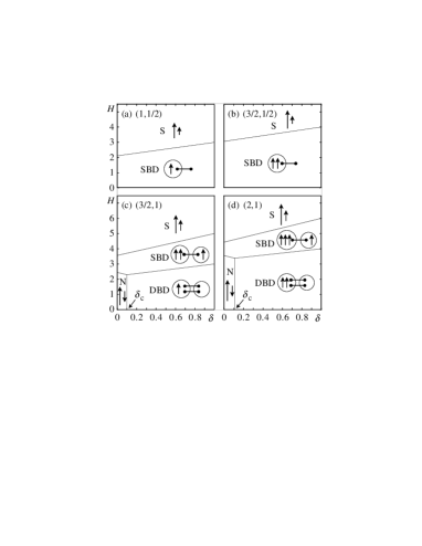
FIG. 3.: The variational ground-state phase diagrams on the $\delta H$-plane for the Hamiltonian (2) with $\alpha=1$ at various values of $(S,s)$.

In order to characterize the plateaux, we introduce a variational wave function for the ground state of the model (3) as

$$|{\rm g}\rangle=c_{\rm N}\prod_{j=1}^{N}(A_{j}^{\dagger})^{2S}(b_{j}^{\dagger})^{2s}|0\rangle$$ (7)

$$\ +\sum_{l=0}^{2s}c_{\rm VB}^{(l)}\prod_{j=1}^{N}(A_{j}^{\dagger})^{2S-l}(a_{j}^{\dagger})^{2s-l}(A_{j}^{\dagger}b_{j}^{\dagger}-B_{j}^{\dagger}a_{j}^{\dagger})^{l}|0\rangle\,,$$ (8)

where $c_{\rm N}$ and $c_{\rm VB}^{(l)}$ are the mixing coefficients. Since all the elemental states are asymptotically orthogonal to each other, the thermodynamic-limit variational ground states are considerably simple, as shown in Fig. 3, where we consider the Heisenberg point. The phase diagrams are exact on the line of $\delta=1$, where the spin-$(\frac{3}{2},1)$ chain, for example, reaches the saturation (S) via the double-bond dimer (DBD) and single-bond dimer (SBD) states. The point is that the $\delta=0$ ground states are better approximated by the decoupled-dimer states than by the Néel (N) states in the cases of $s=\frac{1}{2}$, while vice versa in all other cases. For $s=\frac{1}{2}$, the variational wave function (8) ends up with $c_{\rm N}=0$ all over the $\delta$-$H$ plain. The Néel-dimer crossover point $\delta_{\rm c}$ is given by

$$\delta_{\rm c}=\frac{2Ss-A+B+C}{A-B+C}\,,$$ (9)

with

$$A=\sum_{l=1}^{2s}\biggl{\{}\frac{(2S-2s+l)!(2S-2s+l-1)!}{[(2S-2s)!]^{2}l!(l-1)!}$$ (10)

$$\qquad\times[S(S+1)-(S-2s+l-1)(S-2s+l)]$$ (11)

$$\qquad\times[s(s+1)-(s-l)(s-l+1)]\biggr{\}}^{1/2}$$ (12)

$$\qquad/\sum_{l=0}^{2s}\frac{(2S-2s+l)!}{(2S-2s)!l!}\,,$$ (13)

$$B=\sum_{l=0}^{2s}\frac{(2S-2s+l)!}{(2S-2s)!l!}(S-2s+l)(s-l)$$ (14)

$$\qquad/\sum_{l=0}^{2s}\frac{(2S-2s+l)!}{(2S-2s)!l!}\,,$$ (15)

$$C=\sum_{l=0}^{2s}\frac{(2S-2s+l)!}{(2S-2s)!l!}(S-2s+l)$$ (16)

$$\qquad\times\sum_{l=0}^{2s}\frac{(2S-2s+l)!}{(2S-2s)!l!}(s-l)$$ (17)

$$\qquad/\sum_{l=0}^{2s}\frac{(2S-2s+l)!}{(2S-2s)!l!}\,.$$ (18)

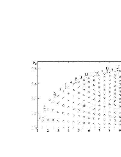
FIG. 4.: The variational crossover points $\delta_{\rm c}$ between the Néel-ordered state and the $2s$-bond decoupled-dimer state for the Hamiltonian (2) with $\alpha=1$ at various values of $(S,s)$.

$\delta_{\rm c}$ does not exist for $s=\frac{1}{2}$, whereas it is an increasing function of $s$ for $s\geq 1$, as shown in Fig. 4. Thus, the Néel-gap-like character of the initial plateaux in the multi-step magnetization curves become more and more settled as $s$ increases, which leads to the instability of the plateaux against the $XY$-like anisotropy. The exceptional cases of $s=\frac{1}{2}$ may be recognized as the quantum limit. Another simple calculation also supports this scenario. Let us consider a spin-wave description and a perturbation treatment of the antiferromagnetic excitation gap from the ground state. The spin-wave excitations are based on the Néel-order background, whereas the perturbation from the decoupled-dimer limit assumes the crackion-like excitations to appear in the valence-bond background. We compare in Table I both estimates with the exact values, namely, the upper critical fields for the initial plateaux. In the cases of $s=\frac{1}{2}$, the perturbation calculations are better than the spin-wave estimates, while vice versa in the cases of $s\geq 1$. We are again convinced that the single plateaux for $s=\frac{1}{2}$ are relatively of quantum aspect, while the lowest-magnetization plateaux in the multi-step process for $s\geq 1$ are relatively of classical aspect. All other plateaux, the second and higher steps, should essentially be based on the quantum mechanism. Now here is a question: As $\alpha$ increases, at which point do the quantum plateaux for $m>S-s$ disappear? Our numerical investigations estimate that they survive the whole region of $\alpha>1$ and disappear in the Ising limit.

Finally we draw the ground-state phase diagrams on the $\alpha\delta$-plane. If the system is massive at the sector of magnetization $M$, $H_{\pm}(N,M)$ are extrapolated to different thermodynamic-limit values $H_{\pm}(m)$ with exponential size corrections. On the other hand, in the critical phase, $H_{\pm}(N,M)$ converge to the same value as [47, 48]

$$H_{\pm}(N,M)\sim H(m)\pm\frac{\pi v_{\rm s}\eta}{N}\,,$$ (19)

where $v_{\rm s}$ is the spin-wave velocity and $\eta$ is the critical index for the relevant spin-correlation function. Therefore, we can visualize the phase transition by plotting the scaled gap $N{\mit\Delta}_{N}(m)$ as a function of $\alpha$ as shown in Fig. 5. The phase boundaries could in principle be extracted

FIG. 5.: Scaled quantity $N{\mit\Delta}_{N}(m)$ versus $\alpha$ at $m=\frac{1}{2}$ (a) and $m=\frac{3}{2}$ (b) in the case of $(S,s)=(\frac{3}{2},1)$.

FIG. 6.: The ground-state phase diagrams on the $\alpha\delta$-plane for the Hamiltonian (2) at various values of $(S,s)$.

from the phenomenological renormalization-group equation [49] taking ${\mit\Delta}_{N}(m)$ as the order parameter. However, the anisotropy-induced breakdown of the plateau is a transition of the Kosterlitz-Thouless type and the fixed point could only be determined with great uncertainty [50]. Thus we here rely upon the critical exponent $\eta$ which should cross over the value $\frac{1}{4}$ on the phase boundary. Provided $v_{\rm s}$ is given, we can estimate $\eta$ using the scaling law (19). We obtain $v_{\rm s}$ directly from the dispersion relation. Using the scaling relation [47, 48]

$$\frac{E(N,M)}{N}\sim\varepsilon(m)-\frac{\pi cv_{\rm s}}{N^{2}}\,,$$ (20)

we further verify the central charge being unity in the critical region, though it is not so useful in determining the phase boundary. The thus-obtained phase boundaries are shown by solid lines in Fig. 6. The single plateaux, with a quantum base, are stable over the whole antiferromagnetic-coupling region (a,b), while the initial plateaux in the multi-step process, taking on a classical character, less survive the $XY$-like anisotropy than the quantum higher plateaux (c,d). The existence of the second plateaux without any bond polymerization, which is the main issue in the present article, should be verified very carefully. So then we further employ an idea of the level spectroscopy [51], thus called, in analyzing the second plateau. Comparing the relevant excitation energies whose scaling dimensions are $2$ at the critical point, we recognize the level crossing of them as the phase boundary. The thus-detected transitions are also plotted by broken lines in Fig. 6. The slight difference between the two estimates inevitably arises from the logarithmic corrections to the scaling law (19), where the level spectroscopy is more reliable than the naivest scaling analysis. Anyway, we may now fully be convinced of the existence of the novel multi-plateau magnetization curves.

IV Summary and Future Aspect

The one-dimensional Heisenberg ferrimagnet with alternating spins $S$ and $s$ exhibits a $2s$-plateau magnetization curve even at the most symmetric point. It is interesting to compare the present spin-$(S,s)$ ferrimagnetic chain with the spin-$\frac{1}{2}$ bond-polymerized chain of period $2(S+s)$, that is, the $(2S-1)$-times-ferromagnetic-antiferromagnetic-$(2s-1)$-times-ferromagnetic-antiferromagnetic chain. In the strong ferromagnetic-coupling limit, the latter may be regarded as equivalent to the former. In the same meaning, the spin-$S$ antiferromagnetic Heisenberg chain can be viewed as a spin-$\frac{1}{2}$ bond-polymerized chain of period $2S$. Such replica chains generally exhibit magnetization plateaux in certain regions of the ratio of the ferromagnetic coupling $J_{\rm F}$ to the antiferromagnetic one $J_{\rm A}$, $\gamma\equiv J_{\rm F}/J_{\rm A}$. However, in the case of the spin-$\frac{1}{2}$ ferromagnetic-ferromagnetic-antiferromagnetic chain which is the replica model of the spin-$\frac{3}{2}$ antiferromagnetic Heisenberg chain, Okamoto [6] and Hida [7] reported that the plateau vanishes at $\gamma=4\sim 5$ and therefore the pure Heisenberg chain exhibits no plateau. Thus the plateaux observed here in the most symmetric Heisenberg ferrimagnets still interest us to a great extent.

As we come up the steps, the plateau length exponentially decreases. It is hard to numerically observe the higher-lying plateaux, still harder experimentally. Only the first and second plateaux may lie within the limits of measurement. In this context, we are fortunate to have a series of bimetallic quasi-one-dimensional complexes MM^′(EDTA)$\cdot$6H₂O ($\mbox{M},\mbox{M}^{\prime}=\mbox{Mn},\mbox{Co},\mbox{Ni},\mbox{Cu}$) [52]. Their exchange coupling constants are all about $10k_{\rm B}$[K] and thus the complete magnetization curves could technically be observed. Magnetization measurements on them, especially with $\mbox{M}=\mbox{Mn}\,(S=\frac{5}{2}),\mbox{Co}\,(S=\frac{3}{2})$ and $\mbox{M}^{\prime}=\mbox{Ni}\,(s=1)$, are encouraged. The plateaux would more or less be obscured in any actual measurement, but they, however small, should necessarily be detected by some anomaly in the magnetic susceptibility. The chemical modification of the bond alternation $\delta$ and/or the exchange anisotropy $\alpha$ must help us to directly observe the second-step plateaux, though we take main interest in the Heisenberg point.

TABLE I.: Estimates of the antiferromagnetic excitation gap from the ground state for the Hamiltonian (2) with $\alpha=1$ and $\delta=0$ by the use of the linear spin-wave theory (spin wave), the perturbation from the decoupled-dimer limit (perturbation), and the exact diagonalization (exact).

$(S,s)$	spin wave	perturbation	exact
$(1,\frac{1}{2})$	$1$	$\frac{11}{9}$	$1.759(1)$
$(\frac{3}{2},\frac{1}{2})$	$2$	$\frac{17}{8}$	$2.842(1)$
$(\frac{3}{2},1)$	$1$	$\frac{16}{45}$	$1.615(10)$
$(2,1)$	$2$	$\frac{11}{30}$	$2.730(5)$