On the existence of a variational principle for deterministic cellular automaton models of highway traffic flow

Keywords: cellular automata, interacting particles, highway traffic models, variational principle.

Abstract. It is shown that a variety of deterministic cellular automaton models of highway traffic flow obey a variational principle which states that, for a given car density, the average car flow is a non-decreasing function of time. This result is established for systems whose configurations exhibits local jams of a given structure. If local jams have a different structure, it is shown that either the variational principle may still apply to systems evolving according to some particular rules, or it could apply under a weaker form to systems whose asymptotic average car flow is a well-defined function of car density. To establish these results it has been necessary to characterize among all number-conserving cellular automaton rules which ones may reasonably be considered as acceptable traffic rules. Various notions such as free-moving phase, perfect and defective tiles, and local jam play an important role in the discussion. Many illustrative examples are given.

1 Introduction

The publication of the Nagel-Schreckenberg highway traffic flow cellular automaton (CA) model [1] has attracted much interest. Since then, many papers describing various CA models of traffic flow have been published [2, 3, 4, 5, 6]. Most results concerning the properties of traffic flow models have been obtained with the help of either numerical simulations or various extensions of the mean-field approximation. Only few exact results are known. In the case of the Fukui-Ishibashi (FI) model [3], which is a natural extension of Wolfram’s Rule 184 [7], Fukś [8] has recently derived the exact expression of the average car flow as a function of time. This result shows that, in the infinite lattice size limit, the average car flow is a monotonous increasing function of time. That is, the FI model (and Rule 184 to which it reduces if the speed limit is equal to 1) obeys a variational principle. The purpose of this paper is to find out to what extent such a principle remains valid for other deterministic CA models of traffic flow.

2 Rules and configurations representations

In CA models of traffic flow on a circular one-lane highway, the road is represented by a lattice of $L$ cells with periodic boundary conditions. Each cell is either empty (in state 0) or occupied by a car (in state 1). Since the number of cars traveling a circular highway is conserved, such a system evolves according to a number-conserving CA rule. We recently established [9] a necessary and sufficient condition for a one-dimensional $q$-state ($q\geq 2$) deterministic CA rule to be number-conserving, and studied a few illustrative examples. These rules may be seen as deterministic evolution rules of one-dimensional closed systems of interacting particles. Among these rules, some are such that all particles always move in the same direction. All deterministic CA models of highway traffic flow are members of this family of rules.

Although most papers on CA models of traffic flow deal with two-state CA, some number-conserving $q$-state CA rules, with $q>2$, can also be good candidates [10]. In this case, a cell could, for instance, either represent a longer segment of the highway capable of accommodating a maximum of $q-1$ cars or the unit segment of a $(q-1)$-lane highway.

In standard CA modeling it is usually assumed that the configuration at time $t+1$ is entirely determined by the configuration at time $t$. Within this restrictive framework, models like [1, 2] are not standard CA models since the road configuration at time $t+1$ depends on road configurations at time $t$ and $t-1$.

As we shall see, the family of potential models of traffic flow in terms of deterministic one-dimensional two-state standard cellular automata is rather rich, and, in this paper, only models of this type will be considered.

In our discussion of traffic rules, we will not represent CA rules by their rule tables, but make use of a representation which clearly exhibits the particle motion. This motion representation, or velocity rule, which has been introduced in [11], may be defined as follows. If the integer $r$ is the rule’s radius, list all the $(2r+1)$-neighborhoods of a given particle represented by a 1 located at the central site of the neighborhood. Then, to each neighborhood, associate an integer $v$ denoting the velocity of this particle, that is the number of sites this particle will move in one time step, with the convention that $v$ is positive if the particle moves to the right and negative if it moves to the left. For example, Rule 184, defined by

$$f_{184}(0,0,0) =0, \quad f_{184}(0,0,1) =0, \quad f_{184}(0,1,0) =0, \quad f_{184}(0,1,1) =1,$$

$$f_{184}(1,0,0) =1, \quad f_{184}(1,0,1) =1, \quad f_{184}(1,1,0) =0, \quad f_{184}(1,1,1) =1,$$

is represented by the radius-1 velocity rule:

$$\mathtt{\bullet 11}\rightarrow\mathtt{0},\quad\mathtt{\bullet 10}\rightarrow\mathtt{1}.$$ (1)

The symbol $\bullet$ represents either a 0 or a 1, i.e., either an empty or occupied site. This representation, which clearly shows that a car can move to the next-neighboring site on its right if, and only if, this site is empty, is shorter and more explicit.

When discussing road configurations evolving according to various illustrative rules, the knowledge of both car positions and velocities will prove necessary. Therefore, although we are dealing with two-state CA rules, we will not represent the state of a cell by its occupation number (i.e., 0 or 1), but by a letter in the alphabet $\{\mathtt{e,0,1,\ldots,v_{\max}}\}$ indicating that the cell is either empty (i.e., in state $\mathtt{e}$) or occupied by a car with a velocity equal to $\mathtt{v}$ (i.e., in state $\mathtt{v}\in\{\mathtt{0,1,\ldots,v_{\max}}\}$). Note that $\mathtt{v}$ is the velocity with which the car is going to move at the next time step. Configurations of cells of this type will be called velocity configurations or configurations for short.

3 The deterministic FI model of traffic flow

The simplest deterministic CA model of traffic flow is the FI model [3] which might be defined as follows. If $d_{i}(t)$ is the distance, at time $t$, between car $i$ and car $i+1$ (cars are moving to the right), velocities are updated in parallel according to the subrule:

$$v_{i}(t+1)=\min(d_{i}(t)-1,v_{\max})$$ (2)

where $v_{i}(t)$ is the velocity of car $i$ at time $t$; then cars move according to the subrule:

$$x_{i}(t+1)=x_{i}(t)+v_{i}(t+1),$$ (3)

where $x_{i}(t)$ is the position of car $i$ at time $t$. The model contains two parameters: the speed limit $v_{\max}$, which is the same for all cars, and the car density $\rho$.

For the sake of simplicity, in our discussion of this model, it is sufficient to consider the case $v_{\max}=2$. The corresponding radius-2 velocity rule is:

$$\mathtt{\bullet\bullet 11\bullet\rightarrow 0},\quad\mathtt{\bullet\bullet 101\rightarrow 1},\quad\mathtt{\bullet\bullet 100\rightarrow 2}.$$ (4)

Figures 1 and 2 show examples of spatiotemporal patterns for car densities $\rho$, respectively, equal to 0.26 and 0.50. Empty cells are white while cells occupied by a car with velocity $v$ equal to 0, 1, and 2 are, respectively, light grey, dark grey and black.

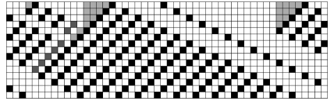
Figure 1: Spatiotemporal pattern of rule (4) for $\rho=0.26$. States color code: white = $e$, light grey = $0$, dark grey = $1$, black = $2$.

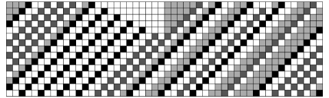
Figure 2: Spatiotemporal pattern of rule (4) for $\rho=0.50$. States color code: white = $e$, light grey = $0$, dark grey = $1$, black = $2$.

According to velocity rule (4), and our choice of configurations representation, a cell occupied by a car with velocity $v$ must be preceded by, at least, $v$ empty cells. Each configuration is, therefore, a concatenation of the following four types of tiles:

2	e	e

1

e

0

e

The first tile, which corresponds to cars moving at the speed limit $v_{\max}=2$, will be called a perfect tile, the next two tiles, corresponding to cars with a velocity less than 2 (here 1 and 0) will be called defective tiles, and the last tile will be called a free empty cell, that is, an empty cell which is not part of either a perfect or defective tile.

Figure 1 shows that only the first configurations contain defective tiles. After a few time steps, these tiles progressively disappear, and the last configurations contain only perfect tiles and free empty cells. Hence, all cars move at $v_{\max}=2$, and the system is said to be in the free-moving phase. In Figure 2, at the beginning, the same process of annihilation of defective tiles takes place but, in this case, all defective tiles do not eventually disappear. A few cars move at $v_{\max}$, while other cars have either a reduced speed ($v=1$) or are stopped ($v=0$). This regime is called the jammed phase. For $v_{\max}>2$, FI models exhibit similar qualitative features.

To analyze the annihilation process of defective tiles in FI models, we need to define what we call a local jam.

Definition 1 In deterministic FI models of traffic flow, a local jam is a sequence of defective tiles preceded by a perfect tile and followed by either a perfect tile or free empty cells.

From this definition, it follows that:

Proposition 1 In the case of deterministic FI models of traffic flow, the number of cars which belong to a local jam is a non-increasing function of time.

This result is a direct consequence of the fact that, by definition, a local jam is preceded by a car which is free to move, and, according to whether a new car joins the local jam from behind or not, the number of cars in the local jam remains unchanged or decreases by one unit. Note that the jammed car just behind the free-moving car leading the local jam becomes itself free to move at the next time step.

In order to establish the variational principle, let analyze more precisely how the structure of the most general local jam changes in one time step. A local jam consisting of $n$ defective tiles is represented below:

$$\cdots v_{1}\underbrace{ee\cdots e}_{v_{1}}v_{2}\underbrace{ee\cdots e}_{v_{2}}\cdots\cdots v_{n}\underbrace{ee\cdots e}_{v_{n}}v_{\max}\underbrace{ee\cdots e}_{v_{\max}}\cdots,$$

where, for $i=1,2,\ldots,n$, $0\leq v_{i}<v_{\max}$. At the next time step, a car with velocity $v_{i}$ located in cell $k$ moves to cell $k+v_{i}$. Hence, if the local jam is followed by $v_{0}$ free empty cells, where $v_{0}\geq 0$, we have to distinguish two cases:

(i) If $v_{0}+v_{1}<v_{\max}$, then the number of jammed cars remains unchanged but the leftmost jammed car, whose velocity was $v_{1}$, is replaced by a jammed car whose velocity is $v_{0}+v_{1}$:

$$\cdots v_{\max}\overbrace{ee\cdots e}^{v_{\max}+v_{0}}v_{1}ee\cdots ev_{2}ee\cdots\ e\cdots\cdots v_{n}ee\cdots ev_{\max}ee\cdots e\cdots$$

$$\cdots e(v_{0}+v_{1})ee\cdots ev_{2}ee\cdots e\cdots\cdots v_{n} ee\cdots ev_{\max}ee\cdots e\cdots$$

(ii) If $v_{0}+v_{1}\geq v_{\max}$, then the local jam loses its leftmost jammed car:

$$\cdots ev_{1}ee\cdots ev_{2}ee\cdots e\cdots\cdot\cdots v_{n}ee\cdots ev_{\max}ee\cdots e\cdots$$

$$\cdots v_{\max}\underbrace{ee\cdots e}_{v_{\max}+v_{0}^{\prime}}v_{2}ee\cdots e\cdots\cdots v_{n} ee\cdots ev_{\max}ee\cdots e\cdots$$

and at the next time step, the local jam is followed by $v_{0}+v_{1}-v_{\max}=v_{0}^{\prime}<v_{0}$ free empty cells.

If we partition the lattice in tiles sequences whose end points are perfect tiles, then, between two consecutive perfect tiles, either there is a local jam, and the above proof shows that the number of free empty cells between the two perfect tiles cannot increase, or there is no local jam, and the number of free empty cells between the two perfect tiles remains unchanged. We can, therefore, state:

Proposition 2 In the case of deterministic FI models of traffic flow, the number of free empty cells is a non-increasing function of time.

Remark 1 If a configuration contains no perfect tiles, then it does not contain free empty cells. Such a configuration belongs, therefore, to the limit set, and as we shall see below, the system is in its steady state. On a circular highway, if a configuration contains only one perfect tile, the above reasoning applies without modification.

Remark 2 The above proof shows that at each time step, the rightmost jammed car of a local jam moves one site to the left. Local jams can only move backwards.

If $L$ is the lattice length, $N$ the number of cars, and $N_{\rm fec}(t)$ the number of free empty cells at time $t$, we have

$$N_{\rm fec}(t)=L-N-\sum_{i=1}^{N}v_{i}(t),$$

since, at time $t$, car $i$ is necessarily preceded by $v_{i}(t)$ empty cells. Dividing by $L$ we obtain

$$\frac{N_{\rm fec}(t)}{L}=1-\frac{N}{L}-\frac{N}{L}\,\frac{1}{N}\sum_{i=1}^{N}v_{i}(t).$$

Hence, for all $t$,

$$\rho_{\rm fec}(t)=1-\rho-\rho\langle v\rangle_{t},$$ (5)

where $\rho_{\rm fec}(t)$ is the density of free empty cells at time $t$, and $\langle v\rangle_{t}$ the average car velocity at time $t$. This last result shows that, when time increases, since the density of free empty cells cannot increase, the average car flow $\rho\langle v\rangle_{t}$ cannot decrease. Deterministic FI models of highway traffic flow obeys, therefore, the following variational principle:

Proposition 3 In the case of deterministic FI models of traffic flow, for a given car density $\rho$, the average car flow is a non-decreasing function of time and reaches its maximum value in the steady state.

The annihilation process of defective tiles stops when there are either no more defective tiles or no more free empty cells. Since a perfect tile consists of $v_{\max}+1$ cells, if the car density $\rho$ is less than $\rho_{c}=1/(v_{\max}+1)$, there exist enough free empty cells to annihilate all the defective tiles, and all cars become eventually free to move. If $\rho>\rho_{c}$, there are not enough free empty cells to annihilate all defective tiles, and eventually some cars are not free to move at $v_{\max}$. The threshold value $\rho_{c}$ is called the critical density. At the end of the annihilation process, all subsequent configurations belong to the limit set, and the system is either said to be in equilibrium or in the steady state.

Note that the existence of a free-moving phase for a car density less than $\rho_{c}=1/(v_{\max}+1)$, can be seen as a consequence of Relation (5). When $t$ goes to infinity, according to whether $\rho_{\rm fec}$ is positive or zero, this relation implies

$$\langle v\rangle_{\infty}=\min\left(\frac{1-\rho}{\rho},v_{\max}\right).$$

If the system is finite, its state becomes eventually periodic in time, and the period is equal to the lattice size or one of its submultiples.

Since local jams move backwards and free empty cells move forwards, equilibrium is reached after a number of time steps proportional to the lattice size.

Remark 3 In the case of Rule 184, the existence of a free-moving phase for a particle density $\rho$ less than the critical density $\rho_{c}=\frac{1}{2}$, obviously implies that the average velocity $\langle v\rangle_{t}$, as a function of time $t$, is maximum when $t\to\infty$. For $\rho>\frac{1}{2}$, this property is still true since the dynamics of the holes (empty sites) is governed by the conjugate of rule Rule 184 (i.e., Rule 226), which describes exactly the same dynamics as Rule 184 but for holes moving to the left. Therefore, for all values of the particle density, the average velocity takes its maximum value in the steady state.

In the next section, we shall examine to what extent the variational principle, valid for all deterministic FI traffic flow models, remains valid for more general deterministic CA models of highway traffic flow.

4 Variational principle

In order to extend Proposition 3 to more general deterministic CA models of traffic flow, we have first to characterize, among the class of number-conserving deterministic two-state CA rules, which rules may be considered as acceptable CA traffic rules.

4.1 Unidirectional motion

The first obvious condition to be satisfied by a traffic rule is that all cars should move in the same direction, that is, in the motion representation, all velocities should have the same sign.

Example 1 For instance, the rule:

$$\mathtt{\bullet 011\bullet}\rightarrow\mathtt{-1},\quad\mathtt{\bullet 111\bullet}\rightarrow\mathtt{0},\quad\mathtt{\bullet\!\bullet\!101}\rightarrow\mathtt{0},\quad\mathtt{\bullet\!\bullet\!100}\rightarrow\mathtt{1}$$ (6)

is not acceptable since a particle can move either to the right or to the left. Many number-conserving CA rules are not unidirectional. In the case of (6), it can be shown [11] that each particle performs a non-Gaussian pseudo-random walk. The rule being deterministic, the randomness comes from the randomness of the initial configuration.

4.2 Existence of a free-moving phase

The second natural condition, which should be satisfied by a deterministic CA traffic rule, is that, when the car density is sufficiently low, each car should eventually be able to move at the speed limit $v_{\max}$.

Example 2 A numerical simulation of a one-dimensional system of particles evolving according to the rule:

$$\mathtt{\bullet\!\bullet\!11\bullet\rightarrow 0},\quad\mathtt{\bullet 1101\rightarrow 1},\quad\mathtt{\bullet 010\,\bullet\rightarrow 1},\quad\mathtt{\bullet 1100\rightarrow 2}$$ (7)

shows that, for a particle density $\rho<\frac{1}{2}$, all particles eventually move at $v=1$. For $\rho>\frac{1}{2}$, the asymptotic average velocity decreases monotonically and goes to zero for $\rho=1$. This rule is, however, not an acceptable traffic rule. The velocity of a particle can be equal to $v_{\max}=2$ only if there is another particle located just behind (i.e., on its left) whose velocity is zero. This implies that, while $v_{\max}=2$, the average velocity cannot be larger than 1. The regime in which all particles move at the same velocity $v=1$ is not a true free-moving phase.

Example 3 It is often necessary to look closely at the velocity rule to tell if a system of particles evolving according to such a rule exhibits a free-moving phase at low density. Consider, for instance, the rule:

$$\mathtt{1\!\bullet\!11\bullet\rightarrow 0},\quad\mathtt{0111\bullet\rightarrow 0},\quad\mathtt{001\!\bullet\!\bullet\rightarrow 0},$$

$$\qquad\quad\mathtt{1\!\bullet\!10\,\bullet\rightarrow 1},\quad\mathtt{0110\,\bullet\rightarrow 1}.$$ (8)

The rule elements $\mathtt{1\!\bullet\!10\,\bullet\rightarrow 1}$ and $\mathtt{0110\,\bullet\rightarrow 1}$ indicate that, if the particle density is too low, no motion can probably take place. Actually, a simple numerical simulation shows that below $\rho_{\min}=\frac{1}{3}$, the asymptotic average velocity is always zero. More precisely, it can be shown that, in the steady state, if $\rho_{v}$ denotes the fraction of all particles whose velocities is equal to $v$, there exist three regimes:

(i) If $\rho\leq\frac{1}{3}$, then $\rho_{0}=\rho$.

(ii) If $\frac{1}{3}\leq\rho\leq\frac{1}{2}$, $\rho_{0}$ and $\rho_{1}$ satisfy the relations:

$$\rho_{0}+\rho_{1}=\rho,\quad\mbox{and}\quad 3\rho_{0}+2\rho_{1}=1,$$

that is,

$$\rho_{0}=1-2\rho,\quad\mbox{and}\quad\rho_{1}=3\rho-1.$$

(iii) If $\frac{1}{2}\leq\rho\leq 1$, $\rho_{0}$ and $\rho_{1}$ satisfy the relations:

$$\rho_{0}+\rho_{1}=\rho,\quad\mbox{and}\quad\rho_{0}+2\rho_{1}=1,$$

that is,

$$\rho_{0}=2\rho-1,\quad\mbox{and}\quad\rho_{1}=1-\rho.$$

A system of particles evolving according to (8) does not exhibit a free-moving phase. It is only when $\rho$ is exactly equal to $\frac{1}{2}$ that all particles move at $v_{\max}=1$. As a traffic rule (8) should be discarded.

Example 4 The existence of a free-moving phase for a system of particles evolving according to a given number-conserving deterministic CA rule does not, however, guarantee that such a rule is a reasonable traffic rule. For example, in the case of the velocity rule:

$$\mathtt{\bullet\bullet\bullet 111\,\bullet\rightarrow 0},\quad\mathtt{\bullet\bullet\bullet 1101\rightarrow 1},\quad\mathtt{\bullet\bullet\bullet 1011\rightarrow 1},$$

$$\mathtt{\bullet\bullet\bullet 1100\rightarrow 2},\quad\mathtt{\bullet\bullet\bullet\,1010\rightarrow 2},\quad\mathtt{\bullet\bullet\bullet 100\,\bullet\rightarrow 2},$$ (9)

all velocities have the same sign, and a simple numerical simulation shows that, below a critical density equal to $\frac{1}{2}$, there exists a free-moving phase in which all the particles move with the velocity $v_{\max}=2$. Its flow diagram has even a nice tent-shape. But, as a traffic rule, (9) shows that drivers are anticipating the motion of cars on their right [5]. Since all drivers move according to the same rule, no collisions occur. But, to make traffic rules somewhat more realistic, most authors [1, 3, 12] consider essential to add some randomization, as random braking, to the basic deterministic model. In the case of rule (9) this would lead to collisions, whose number would increase with the braking probability. Moreover, at the critical density, systems evolving according to a deterministic car traffic rule exhibit a second-order phase transition, and it has been recently shown [13] that, for traffic flows evolving according to FI traffic rules, random braking is the symmetry-breaking field conjugate to the order parameter defined as $m=v_{\max}-\langle v\rangle_{\infty}$. For all these reasons, we should not accept as a traffic rule any deterministic CA rule in which a particle can move to an occupied site “knowing” that the particle located at that site will also move.

In the light of the preceding examples, we shall adopt the following definition of a free-moving phase

Definition 2 A system of particles evolving according to a unidirectional deterministic CA rule exhibits a free-moving phase if there exists a number $0<\rho_{c}<1$, called the critical density, such that, starting from a random configuration with a particle density $\rho<\rho_{c}$, the system evolves to an equilibrium state in which, with probability one, all configurations consists of perfect tiles and free empty cells. If the maximum velocity at which a particle can move is $v_{\max}$, a perfect tile consists of a cell in state $v_{\max}$ preceded by $v_{\max}$ empty cells.

Example 5 The structure of the last element of the velocity rule:

$$\mathtt{\bullet\!\bullet\!11\bullet\rightarrow 0},\quad\mathtt{1010\,\bullet\rightarrow 0},\quad\mathtt{0010\,\bullet\rightarrow 1},\quad\mathtt{\bullet 1101\rightarrow 1},\quad\mathtt{\bullet 1100\rightarrow 2}$$ (10)

shows that the average velocity can never be equal to $v_{\max}=2$. A system of particles evolving according to such a rule cannot, therefore, exhibit a free-moving phase in the sense of the above definition. This type of result is general: If a particle can move at $v_{\max}$ if, and only if, the site located immediately behind it has to be occupied by another particle, then no free-moving phase in the sense of Definition 2 can exist.

Example 6 The velocity rule:

$$\mathtt{\bullet\bullet\bullet 11\,\bullet\,\bullet\rightarrow 0},\quad\mathtt{\bullet\bullet\bullet 101\,\bullet\rightarrow 0},\quad\mathtt{\bullet\bullet\bullet 1001\rightarrow 1},\quad\mathtt{\bullet\bullet\bullet 1000\rightarrow 2}$$ (11)

describes the behavior of overcautious drivers who avoid occupying a site located just behind another car. The perfect tile:

2	e	e	e

has not the structure required by Definition 2. It contains an extra empty cell. While it could be reasonable to consider models of traffic flows in which some drivers could have an overcautious behavior, if all drivers behave in the same way, then all cars will stop for a density less than the maximum car density $\rho=1$. We will, therefore, not consider such a driving strategy acceptable for deterministic CA traffic rules.

4.3 Local jams

The existence of a free-moving phase implies the existence of a mechanism making possible the annihilation of all local jams. For deterministic FI models, the jammed car just behind the free-moving car leading the local jam becomes free to move at the next time step. If, at low density, we want local jams to gradually disappear, this condition, which was automatically satisfied in the case of deterministic FI traffic flow models, should be required for models evolving according to unidirectional number-conserving deterministic CA rules to be acceptable traffic rules.

Definition 3 A system of particles evolving according to a unidirectional velocity rule is a deterministic traffic flow model if a sequence of defective tiles cannot be preceded by free empty cells. A sequence of defective tiles preceded by a perfect tile is called a local jam.

Proposition 1 can then be extended to all deterministic traffic flow CA models as defined above.

Proposition 4 In a deterministic CA model of traffic flow, the number of cars belonging to a local jam is a non-increasing function of time.

Example 7 A system of particles evolving according to the velocity rule:

$$\mathtt{\bullet\!\bullet\!11\bullet\rightarrow 0},\quad\mathtt{\bullet 0101\rightarrow 0},\quad\mathtt{\bullet 110\bullet\rightarrow 1},\quad\mathtt{\bullet 0100\rightarrow 2}$$ (12)

is not a traffic flow model. All configurations are concatenations of the following three types of tiles and free empty cells:

2	e	e

0

1

e

0

e

The first tile is the perfect tile while the other two tiles are the only defective tiles. Since to move at $v_{\max}=2$ a particle needs not only to have two empty sites in front but also one empty site behind, the existence of a defective tile which contains two particles makes that, as shown in the example below, a sequence of defective tiles might be preceded by free empty cells.

time $$t \cdots eeee2ee01e0e2eeee\cdots$$:

time $$t+1 \cdots eeeeee01e01eee2ee\cdots$$:

To avoid this behavior a defective tile should consist of a cell occupied by one particle with velocity $v<v_{\max}$ preceded by $n_{v}$ empty cells, where $v\leq n_{v}<v_{\max}$.

For FI models, the variational principle followed from the particular structure of defective tiles, that is, the number $n_{v}$ of empty cells preceding a cell in state $v$ was always equal to $v$. All models in which defective tiles have this structure will, therefore, verify Proposition 3, and we can state:

Proposition 5 If a deterministic CA traffic rule is such that local jams have the following structure

$$\cdots v_{1}\underbrace{ee\cdots e}_{v_{1}}v_{2}\underbrace{ee\cdots e}_{v_{2}}\cdots\cdots v_{n}\underbrace{ee\cdots e}_{v_{n}}v_{\max}\underbrace{ee\cdots e}_{v_{\max}}\cdots$$

where, for all $i\in\{1,2,\ldots,n\}$, $0\leq v_{i}<v_{\max}$, then, the average car flow $\rho\langle v\rangle_{t}$ is a non-decreasing function of time $t$, and reaches its maximum value in the steady state.

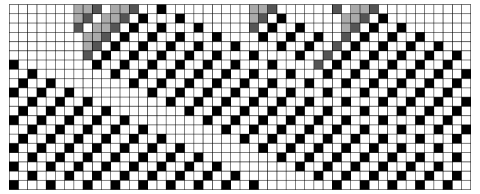
Figure 3: Spatiotemporal pattern of rule (13) for $\rho=0.28$. States color code: white = $e$, light grey = $0$, dark grey = $1$, black = 2.

Example 8 The velocity rule

$$\mathtt{\bullet\bullet 11\bullet\rightarrow 0},\quad\mathtt{\bullet 110\bullet\rightarrow 1},\quad\mathtt{\bullet 0101\rightarrow 1},\quad\mathtt{\bullet 0100\rightarrow 2}$$ (13)

is a nontrivial CA traffic rule satisfying Proposition 5. The speed limit $v_{\max}$ is equal to $2$. As shown in Figure 3, at low density, all cars move at $v_{\max}$. In this regime, the configurations belonging to the limit set consist of perfect three-cell tiles of the type

2	e	e

in a sea of free empty cells. The critical density $\rho_{c}$ is equal to $\frac{1}{3}$.

Figure 4 shows a spatiotemporal pattern for a car density higher than the critical density.

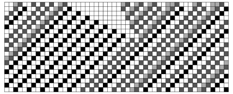
Figure 4: Spatiotemporal pattern of rule (13) for $\rho=0.42$. States color code: white = $e$, light grey = $0$, dark grey = $1$, black = $2$.

All configurations, except the initial configuration chosen at random, are concatenations of perfect tiles, defective tiles, of the following two types:

1

e

0

and free empty cells. Eventually all free empty cells disappear. In both cases, except for the initial configuration, all local jams are such that Proposition 5 applies.

Example 9 There are many nontrivial traffic rules to which Proposition 5 applies. The following traffic rule represents another example:

$$\mathtt{\bullet\!\bullet\!\bullet 11\bullet\!\bullet\rightarrow 0},\quad\mathtt{\bullet\!\bullet\!\bullet\!101\bullet\rightarrow 1},\quad\mathtt{\bullet\!\bullet 01001\rightarrow 2},$$

$$\qquad\quad\mathtt{\bullet\!\bullet\!1100\bullet\rightarrow 2},\quad\mathtt{\bullet\!\bullet 01000\rightarrow 3}$$ (14)

Remark 4 If, as in Example 3, we denote by $\rho_{v}$ the fraction of all particles whose velocities are equal to $v$ in the steady state, for all velocity rules to which Proposition 5 applies, we have

$$\sum_{v=0}^{v_{\max}}\rho_{v} =\rho$$ (15)

$$\sum_{v=0}^{v_{\max}}(v+1)\rho_{v} =1.$$ (16)

Subtracting (15) from (16), we find that the asymptotic average velocity is given by

$$\langle v\rangle_{\infty}=\frac{1}{\rho}\sum_{v=0}^{v_{\max}}v\rho_{v}=\frac{1-\rho}{\rho}.$$

The last expression is exactly the result one obtains using a mean-field argument. The fact that mean-field arguments lead to exact results for CA traffic rules to which Proposition 5 applies has already been found for the values of the critical exponents of phase transitions in FI traffic flow models [13]. It might be conjectured that, for all CA traffic rules to which Proposition 5 applies, critical exponents will be equal to their mean-field values.

Example 10 Proposition 5 does not apply to a system of particles evolving according to the rule:

$$\mathtt{\bullet\!\bullet\!11\bullet\rightarrow 0},\quad\mathtt{\bullet\!\bullet\!101\rightarrow 0},\quad\mathtt{\bullet\!\bullet\!100\rightarrow 2}$$ (17)

since all jammed cars have a zero velocity even when there exists a free empty cell in front. All configurations are concatenations of the following three types of tiles:

2	e	e

0

e

0

and free empty cells. The first tile, which corresponds to cars moving at the speed limit $v_{\max}=2$, is the perfect tile, and the other two tiles, corresponding to cars with a zero velocity are the only defective tiles. It is easy to verify, however, that Proposition 4 apply. Since all jammed cars are stopped cars, it follows that, for a given car density, the average velocity $\langle v\rangle_{t}$ is a monotonous non-increasing function of time.

Example 11 For systems evolving according to the rule:

$$\mathtt{\bullet\!\bullet\!\bullet 11\bullet\!\bullet\rightarrow 0},\quad\mathtt{\bullet\!\bullet\!\bullet\!101\bullet\rightarrow 0},\quad\mathtt{\bullet\!\bullet 01001\rightarrow 1},$$

$$\qquad\quad\mathtt{\bullet\!\bullet\!11001\rightarrow 2},\quad\mathtt{\bullet\!\bullet\!\bullet 1000\rightarrow 3},$$ (18)

due to the existence of defective tiles of the following structures:

1	e	e

0

e

Proposition 5 does not apply, and while Proposition 4 applies, for a given car density, the average velocity $\langle v\rangle_{t}$ is not a monotonous non-increasing functions of time, since, as shown below, the velocity of a jammed car, equal to 1 at time $t$, may become equal to 0 at time $t+1$:

time $$t \cdots 3eee1ee3eeeeee\cdots$$:

time $$t+1 \ \ \cdots ee0e3eeee3eee\cdots.$$:

This example shows that, while a deterministic CA rule may be an acceptable deterministic CA traffic rule, the variational principle, which in its stronger form states that, for a given car density, the average flow is a monotonous non-decreasing function of time, does not apply. The question which could be addressed is then: Is, however, the variational principle still valid under a weaker form?

Since we assumed that a system evolving according to a deterministic CA rule should exhibit a free-moving phase at low car density, by definition of the free-moving phase, all cars move at $v_{\max}$. Therefore, for $\rho<\rho_{c}$, the average car flow takes its maximum value in the steady state. Above the critical density, it is only if the asymptotic average flow is a well-defined function of car density that the question makes sense. If this is the case, then, since Proposition 4 applies to all traffic flow deterministic CA models, it may be reasonably conjectured that, also for $\rho>\rho_{c}$, the average car flow takes its maximum value in the steady state.

Remark 5 This paper deals with the existence of a variational principle for number-conserving deterministic CA models of highway traffic flow. The variational principle, as stated in Proposition 5, may be valid, however, for one-dimensional closed systems of particles evolving according to more general number-conserving deterministic CA rules. For instance, in the case of Rule (7), presented Example 2, all configurations are concatenations of the following three tiles:

0	2	e	e

1

e

0

and free empty cells. The tiles’ structure shows that Relation (5) is valid. If the particle density $\rho$ is less than $\frac{1}{3}$, there are enough free empty cells to annihilate all cells of the first and third type; and all configurations of the limit set are concatenations of tiles of the second type and free empty cells. If $\rho>\frac{1}{3}$, there are not enough free empty cells to annihilate all cells of the first and third type; and all configurations of the limit set contain tiles of all types but no free empty cells. Although such a system does not exhibit a free-moving phase according to Definition 2, cells of the second type play the role of “perfect tiles” while the other two types of cells can be regarded as “defective tiles”.

When Relation (5) is satisfied, it is necessary to verify that the density of free empty cells is a non-increasing function of time to ensure the validity of the variational principle under its stronger form. For instance, while $\rho_{\rm fec}(t)$ cannot increase with time $t$ for a system of particles evolving according to Rule (7), this is no more the case for a system of particles evolving according Rule (10), presented in Example 5, and which is obtained by replacing the element $\mathtt{\bullet 010\bullet\rightarrow 1}$ of Rule (7) by the two elements $\mathtt{1010\bullet\rightarrow 0}$ and $\mathtt{0010\bullet\rightarrow 1}$. As for Rule (7), all configurations are concatenations of the same above three tiles and free empty cells, which implies that Relation (5) is satisfied. But, due the structure of the element $\mathtt{1010\bullet\rightarrow 0}$ of Rule (10), as shown below (three-particle system evolving on a size-10 lattice):

time $$t \underline{ee}02ee1e\underline{ee}$$

time $$t+1 \underline{ee}1e\underline{e}1e0\underline{ee}$$

the number of free empty cells ($\underline{e}$) increases from 4 at time $t$ to 5 at time $t+1$ resulting in a decrease of the average velocity.

5 Conclusion

As illustrated by a number of different examples, many number-conserving deterministic CA rules cannot be considered reasonable deterministic traffic rules, and we tried to list the essential properties characterizing a traffic rule in order to give a general definition of deterministic CA models of highway traffic flow. Various notions such as free-moving phase, perfect and defective tiles, and local jam play an important role in our discussion. We have then shown that, within the framework of this definition, a variety of deterministic CA models of traffic flow obey a variational principle which, in its stronger form, states that, for a given car density, the average car flow is a non-decreasing function of time. This result has been established for traffic flow models whose configurations exhibits local jams of a given structure. If local jams have a different structure, while this variational principle may still apply to systems evolving according to some particular rules, it will not apply in general. However, if the asymptotic average car flow is a well-defined function of car density, since we have proved that for all traffic flow models the number of jammed cars of a local jam cannot increase, we conjectured that it will apply under a weaker form which states that, for a given car density, the average car flow takes its maximum value in the steady state.

The variational principle also applies, even in its stronger form, to many number-conserving deterministic CA rules which cannot be considered reasonable traffic rules.

Acknowledgements

The author is grateful to Henryk Fukś and Andrés Moreira for their very good suggestions. This work has been done during a stay at the Centro de Modelamiento Matemático de la Universidad de Chile in Santiago thanks to FONDAP-CONICYT. The unflagging interest of Eric Goles has been of great help.

References

- [1] K. Nagel and M. Schreckenberg, J. Physique (France) I2 2221 (1992).
- [2] M. Takayasu and H. Takayasu, Fractals 1 860 (1993)
- [3] M. Fukui and Y. Ishibashi, J. Phys. Soc. Japan 65, 1868 (1996)
- [4] T. Tokihiro, D. Takahashi, J. Matsukidaira and J. Satsuma, Phys, Rev. Lett. 76 3247 (1996)
-
[5]
H. Fukś and N. Boccara, Int. J. Mod. Phys. C
9 1 (1998),
(H. Fukś and N. Boccara 1997 Preprint adap-org/9705003). - [6] K. Nishinari and D. Takahashi, J. Phys. A: Math. Gen. 32 93 (1999)
- [7] S. Wolfram S, Cellular Automata and Complexity: Collected Papers (Reading, Massachusetts: Addison-Wesley, 1994).
-
[8]
H. Fukś, Phys. Rev. E 60, 197 (1999),
(H. Fukś 1999 Preprint comp-gas/9902001). -
[9]
N. Boccara and H. Fukś, to appear in Fundamenta
Informaticae,
(N. Boccara and H. Fukś 1997 Preprint cond-mat/9905004). - [10] (K. Nishinari and D. Takahashi 2000 Preprint nlin.AO/0002007
-
[11]
N. Boccara and H. Fukś, J. Phys. A: Math. Gen.,
31 6007 (1998),
(N. Boccara and H. Fukś 1997 Preprint adap-org/9712003). - [12] (A. Schadschneider 1999 Preprint cond-mat/9902170).
-
[13]
N. Boccara and H. Fukś, to appear in volume
33 (2000) of the J. of Phys. A: Math. Gen.,
(N. Boccara and H. Fukś 1999 Preprint cond-mat/9911039).