The spectral properties of noncondensate particles in Bose-condensed atomic hydrogen

Abstract

The strong spin-dipole relaxation, accompanying BEC in a gas of atomic hydrogen, determines the formation of a quasistationary state with a flux of particles in the energy space to the condensate. This state is characterized by a significant enhancement of the low-energy distribution of non-condensate particles, resulting in the growth of their spatial density in the trap. This growth leads to the anomalous reconstruction of the optical spectral properties of non-condensate particles.

The discovery of Bose-Einstein condensation (BEC) in a trapped dilute gas of atomic hydrogen [1, 2] has opened a new page in the studies of metastable gaseous systems at ultracold temperatures. For a long period, trapped atomic hydrogen remained a very promising system to achieve BEC (see, e.g.,[3, 4]). However, only after the involvement of the forced evaporative cooling mechanism typical for the works resulted in the BEC discovery in alkali metal vapors [5, 6, 7] the achievement of BEC in atomic hydrogen became a reality.

The experiments reported in [1, 2] have brought out a set of specific features inherent in the hydrogen system. The anomalously low rate of a three-particle recombination allows one to reach the record density of a Bose condensate of $n_{c}\sim 10^{16}$cm^-3 with the total number of atoms $N$ by several orders of the magnitude greater than that in the experiments on alkali gases. The lightest mass of hydrogen atoms in combination with so high density determines the superfluid phase transition temperature $T_{c}$ exceeding that for the experiments with alkali gases by two orders of the magnitude.

One of most interesting features of the hydrogen experiments is impossibility to achieve a relatively high concentration of the condensate fraction. This result is a direct evidence for the phenomenon of the “burning of a condensate” [8] related to a strong increase of the gas density at the condensation and, as a result, drastic enhancement of the spin relaxation rate (see also [9]). The low rate of the evaporation cooling due to an extremely small scattering length $a\approx 0.65{\rm\stackrel{{\scriptstyle\circ}}{{A}}}$ makes this phenomenon responsible for the kinetics of the formation of a condensate in a gas of atomic hydrogen. This led to the prediction [8] that the concentration of the condensed fraction cannot exceed several percents. It is worthwhile to note that the spatial density of the condensate may be large.

In the experiments [1] an unexpected phenomenon has been observed. The shift of the line of the 1s-2s transition for non-condensate particles is found to increase abruptly after the BEC transition. This is especially surprising since the condensate volume is only about $1\%$ of the volume of the thermal cloud and the estimations presented in [1] could not explain the observed picture. The aim of the present paper is to reveal the nature of this interesting phenomenon.

Under conditions of the experiments [1, 2] the interparticle collision time $\tau$ is small compared with the lifetime of the system $\tau_{L}$. As a result, a quasistationary state sets in for $\tau<t<\tau_{L}$ . For $T>T_{c}$, this state is close to the equilibrium one. However, for $T<T_{c}$ the intense losses of the particles from the condensate due to spin relaxation determine the appearance of the quasistationary state with the compensating flux of particles into the region of low energies. As turns out, the distribution function for the non-condensate fraction of the gas in such state differs drastically from the equilibrium distribution function. An important feature of this “steady-flux” distribution is a sharp increase of the number of particles in the low-energy range of the spectrum. For the trap geometry, this results in a strong increase of the density of normal fraction and therefore causes the anomalous transition line shift for non-condensed atoms. Note that the attempt to explain the anomalous increase of the non-condensate density by introducing a rather artificial model of the formation of metastable dense droplets has recently been undertaken in [10].

We confine ourselves to the time scale of $\tau\ll t\ll\tau_{L}$ and suppose that the quasistationary regime sets in. In order to simplify the analysis we will consider a gas in a spherically symmetric harmonical potential with frequency $\omega$. We suppose that the condensate is in the so-called Thomas-Fermi regime at $T<T_{c}$, that is, $n_{c}(0)U_{0}\gg\hbar\omega$ where $U_{0}=4\pi\hbar^{2}a/m$ and $m$ is the atom mass. This means that the condensate density is determined by the expression

$$n_{c}(r)=\frac{2\mu_{c}-m\omega^{2}r^{2}}{2U_{0}}$$ (1)

valid for $r<r_{\mu}$ where $r_{\mu}=(2\mu_{c}/m\omega^{2})^{1/2}$ and $\mu_{c}=n_{c}(0)U_{0}$ is the chemical potential of the condensate.

At $T<T_{c}$ the loss of the particles is determined mostly by the condensate

$$\dot{n}_{c}(r)=-\frac{1}{2}L^{(2)}n_{c}^{2}(r).$$ (2)

Here $L^{(2)}$ is the spin relaxation coefficient determined for a normal gas and the factor of $1/2$ appears from the two-particle density correlator for a condensate. Note that, in spite of the spatially inhomogeneous loss of Bose-condensed particles, the condensate retains Thomas-Fermi density profile. The point is that the redistribution of particles in the condensate, induced by the mean-field interaction, is much faster than their loss. Indeed, the characteristic evolution time in the condensate is $\tau=\hbar/n_{c}(r)U_{0}$, while the characteristic time of the particle loss is $\tau_{l}=1/L^{(2)}n_{c}(0)$. In the atomic hydrogen $\tau_{l}/\tau\sim 10^{5}$.

With the condensate density distribution (1) we find for the total particle loss rate

$$Q=\frac{16\pi}{105}L^{(2)}n_{c}^{2}(0)r_{\mu}^{3}.$$ (3)

Let us consider the kinetic equation for the normal fraction in a harmonic potential. We are interested in particles with energies $\epsilon>\mu\gg\hbar\omega$. In this case we can disregard the discrete structure of the trap energy levels. Under the assumption of ergodicity the quantum Boltzmann equation acquires the form

$$\dot{n}(\epsilon_{1})=I_{coll}(\epsilon_{1},[n]).$$ (4)

where $n(\epsilon)$ is the statistical average of occupation numbers. Within the energy interval where the occupation numbers are large

$$I_{coll} = W\int_{0}^{\infty}d\epsilon_{2}d\epsilon_{3}d\epsilon_{4}\chi(\epsilon_{1},\epsilon_{2},\epsilon_{3},\epsilon_{4})\delta(\epsilon_{1}+\epsilon_{2}-\epsilon_{3}-\epsilon_{4})$$ (7)

$$\{n(\epsilon_{1})n(\epsilon_{2})[n(\epsilon_{3})+n(\epsilon_{4})]$$

$$-n(\epsilon_{3})n(\epsilon_{4})[n(\epsilon_{1})+n(\epsilon_{2})]\}$$

where

$$\chi(\epsilon_{1},\epsilon_{2},\epsilon_{3},\epsilon_{4})=\left[\min\left(1,\frac{\epsilon_{2}}{\epsilon_{1}},\frac{\epsilon_{3}}{\epsilon_{1}},\frac{\epsilon_{4}}{\epsilon_{1}}\right)\right]^{2},$$ (8)

$$W=\frac{4ma^{2}}{\pi\hbar^{3}}.$$ (9)

This kinetic equation differs from that for a homogeneous case (see, e.g., [11, 12]) only by the exponent in expression (8) (see, e.g., [13, 14]), which is characteristic for a harmonic potential. As we will see below, the increase of spatial density, accompanying BEC, comes from the energy region where $n(\epsilon)\gg 1$. We took the latter condition into account explicitly, deriving Eq. (7).

The density in the energy space can be written as $\rho_{\epsilon}=g(\epsilon)n(\epsilon)$ where $g(\epsilon)=\epsilon^{2}/2(\hbar\omega)^{3}$ is the density of states in the harmonic potential. We can rewrite Eq. (4) in the form of the continuity equation for the energy space

$\displaystyle\frac{\partial\rho_{\epsilon}}{\partial t}=-\frac{\partial}{\partial\epsilon}P(\epsilon)$

with the flux $P(\epsilon)$

$$P(\epsilon)=\int^{\epsilon}d\epsilon^{\prime}g(\epsilon^{\prime})I_{coll}(\epsilon^{\prime},[n]).$$ (10)

In the quasistationary regime $P(\epsilon)=Q=const$. This means that the flux (10) has the same value for an arbitrary $\epsilon$. Taking into account Eq. (7), this requirement can be fulfilled if the distribution function has the form

$$n(\epsilon)=\frac{A}{\tilde{\epsilon}^{\gamma}}$$ (11)

where $\tilde{\epsilon}=\epsilon/\hbar\omega$. Let us substitute this distribution function into Eq. (7). Introducing dimensionless variables $\xi_{i}=\epsilon_{i}/\epsilon_{1}$, after simple transformations we find

$\displaystyle I_{coll}=W(\hbar\omega)^{2}A^{3}I_{0}(\gamma)\tilde{\epsilon}_{1}^{2-3\gamma}$

where

$$I_{0}(\gamma) = \int_{0}^{\infty}d\xi_{2}d\xi_{3}d\xi_{4}\chi(\xi_{2},\xi_{3},\xi_{4})\delta(1+\xi_{2}-\xi_{3}-\xi_{4})$$ (13)

$$(\xi_{4}^{\gamma}+\xi_{3}^{\gamma}-\xi_{2}^{\gamma}-1)(\xi_{2}\xi_{3}\xi_{4})^{-\gamma}$$

Inserting these relations into Eq. (10), we find for the flux

$\displaystyle P(\epsilon)\propto\frac{I_{0}(\gamma)}{5-3\gamma}\epsilon^{5-3\gamma}.$

The requirement of the independence of the flux on $\epsilon$ leads to

$$\gamma=\frac{5}{3}$$ (14)

and simultaneously to $I_{0}(\gamma)=0$. The last result is fairly evident: $I_{coll}$ is equal to zero in a stationary case. At the same time the derivative $I_{0}^{\prime}(\gamma)$ is finite and provides the permanent flux $P=Q$ to the low energies region. The obtained results are in correspondence with the general analysis of Zakharov (see [16] and also [17]), showing that the equation $I_{coll}=0$ has a nontrivial solution relevant to a steady-state particle flux in the energy space.

For the relation between $A$ and $Q$, we obtain

$$A=C\left(\frac{Q}{W(\hbar\omega)^{2}}\right)^{1/3}.$$ (15)

One can estimate the dimensionless numerical coefficient $C$ using the total number of non-condensate particles $N_{nc}$ if one assumes approximately that Eqs. (11),(14) remain valid up to the maximum energy.

It is worth to note that the numerical calculations of the BEC kinetics demonstrate the formation of the distribution of the form (11) (with $\gamma>1$) before the real growth of condensate starts (see, e. g., [12, 15]).

Using $n(\epsilon)$ from Eq. (11), one can find the spatial density distribution $n(r)$ for the normal fraction. The direct numerical calculation shows that the main contribution to $n(r)$ comes from the energy levels $\mu\ll\epsilon<T$. These levels are weakly affected by the presence of the condensate (the volume occupied by the wavefunctions of a particle is much larger than the condensate volume) and by the interparticle interaction in the thermal cloud. This means that within a reasonable approximation we can neglect the renormalization of the levels and use oscillator vavefunctions $\psi_{\mathbf{p}}(\mathbf{r})$ where ${\bf p}\equiv(n_{r},l,m)$. The energy region $(\epsilon-\mu)\sim\mu$, where the modification of the level structure is noticeable, gives a negligible contribution to the spacial density, and we ignore this modification. Under the assumption of ergodicity

$$n({\bf r})=\sum_{\mathbf{p}}|\psi_{\mathbf{p}}({\bf r})|^{2}n(\epsilon_{\mathbf{p}})$$ (16)

Since the spacial density of the thermal cloud is weakly sensitive to the low energies, at the presence of the condensate we simply truncate the sum (16) by the condition $\epsilon_{\mathbf{p}}\geq\mu_{c}$.

Since the concentration of the condensate fraction is confined to several percents, the main part of the particles at $T<T_{c}$ is in the non-condensate fraction and $N_{nc}\approx N$. At $T>T_{c}$ the distribution function for low energies at the actual absence of the flux compensating losses has an equilibrium form $n(\epsilon)=T/(\epsilon+|\mu|)$. Comparing this distribution with Eqs. (11,14), one can see that the maximum density of the non-condensate fraction, determined in the trap mostly by the low-energy region in the presence of flux at $T<T_{c}$, can exceed significantly the equilibrium value of the density at $T>T_{c}$. Note that in the presence of condensate the thermal equilibrium is absent and therefore the temperature may be regarded only as a characteristic energy scale for the system.

For the Doppler-free two-photon excitation, the spectral distribution is determined by the red shift of the absorption line. The shift is caused by the change of the coupling (scattering length) of an excited atom compared with the atom in the ground state. In the quasiclassical approximation the shift is proportional to the local density of particles, coinciding with $n(r)$ beyond the condensate region. Thus, the appearance of a condensate, accompanied by a sharp growth of $n(r)$ for small $r$, causes a significant increase of the shift of the non-condensate spectral distribution.

For an optically thin sample, in the local density approximation the Doppler-free spectral distribution for the two-photon absorption is proportional to the density distribution $G(n)$. For the spherically symmetric configuration, this distribution reads

$$G(n)=4\pi r^{2}(n)\left|\frac{dr(n)}{dn}\right|n$$ (17)

where $r(n)$ is determined from condition $n(r)=n$. For the non-condensate fraction, $n(r)$ is determined by (16).

Below we present approximate quantitative estimations for the described picture on the basis of the experimental data [1, 2]. Since in the experiments the collision time $\tau\sim 10^{-3}$s is much less than the lifetime of the system $\tau_{L}\sim 5$s, the quasistationary regime sets in for times $\tau\ll t\ll\tau_{L}$ as explained above. The maximum condensate density is found to be $n_{c}(0)\approx 5\times 10^{15}$cm^-3. We will consider a spherically symmetric harmonic trap with $\omega=(\omega_{\perp}^{2}\omega_{z})^{1/3}=3.4\times 10^{3}$Hz. Here $\omega_{\perp}$ and $\omega_{z}$ are the frequencies of the cylindrical trap used in [1, 2]. For $L^{(2)}=1.1\times 10^{15}$cm³/s and $a=0.65{\rm\stackrel{{\scriptstyle\circ}}{{A}}}$ [2, 18], we find $Q=1.9\times 10^{9}$s^-1 for the particle loss rate. In the Thomas-Fermi approximation, the number of particles in the condensate for the given parameters is $N_{c}\approx 1.2\times 10^{9}$. The largest uncertainty in the experimental data [1] is related to the value of the relative condensate fraction $\chi$. Here we use some average value of $\chi\approx 0.07$. Then the total number of particles is $N\approx 1.7\times 10^{10}$. The critical temperature of the BEC transition is $T_{c}\approx 60\mu$K in this case.

Let us assume that non-condensate particles are concentrated within the energy interval $[\mu,\epsilon^{*}]$, having distribution (11). Comparing the energies of a system with the distribution (11) and with the equilibrium distribution at temperature $T$, we find $\epsilon^{*}=4.7T_{c}(T/T_{c})^{4}$ for the same number of particles in the both cases. The parameter $\epsilon^{*}\gg\mu$. The increase of the spatial density of non-condensed particles originates from the occupation of the energy interval where $\epsilon$ is significantly smaller than $\epsilon^{*}$. The results are only weakly sensitive to the behavior of $n(\epsilon)$ near the upper bound of the energy spectrum. Our approximate definition of $\epsilon^{*}$ is made with the aim to compare the results below and above $T_{c}$, assuming the same number of particles. Taking into account the estimated values of $N_{nc}$, $Q$ and $W$ from Eq.(9) we can determine the coefficients of $A$ and $C$ in (14,15). At $T\approx 0.9T_{c}$ we obtain $A\approx 2.9\times 10^{5}$ and $C\approx 2.5$.

Using distribution function (11) with the values found for $A$ and $\epsilon^{*}$, one can determine the spatial density distribution (16) for the non-condensate fraction.

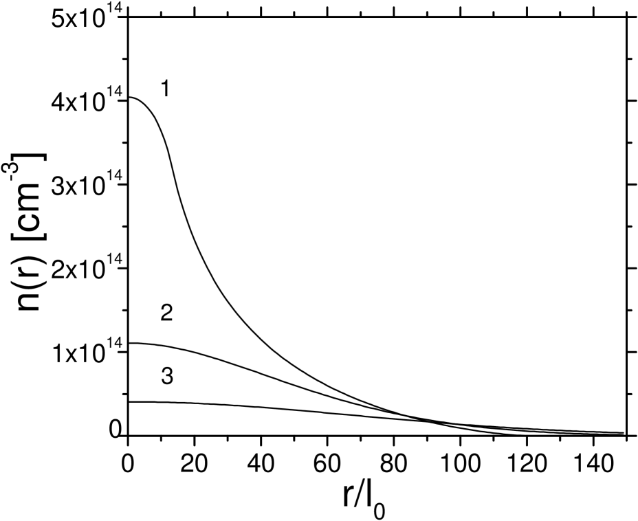
FIG. 1.: The spatial density distribution for the non-condensate fraction ($N=1.7\times 10^{10}$ and $T_{c}=60\mu$K): $T_{1}=0.9T_{c}$ (curve 1), $T_{2}=70\mu$K (curve 2) and $T_{3}=120\mu$K (curve 3).

FIG. 2.: The spectral distribution of two-photon absorption for the non-condensate fraction. The parameters are the same as in FIG.1

The dependence $n(r)$ is shown in FIG.1 (curve 1). For comparison, we present the density profiles for two temperatures above $T_{c}$: 70$\mu$K (curve 2) and 120$\mu$K (curve 3). The length in the figure is given in units of the characteristic trap size $l_{0}=\sqrt{\hbar/m\omega}$. The absence of condensate at $T>T_{c}$ allows one to neglect the spin relaxation losses and therefore to use the equilibrium distribution with the chemical potential fixing the same number of particles.

Knowing $n(r)$, we can find $G(n)$ (17) and therefore the spectral distribution of two-photon absorption. To make a comparison with the experimental results [1], we use the relation $\Delta\nu(n)=\eta n$ for the shift of absorption line and, according to [1], assume that the coefficient $\eta$ has the same value both for the condensate and for the non-condensate fraction. Regardless of a specific value of the scattering length for the interaction between an excited atom and atoms in the ground state, one can use the relation $\Delta\nu(n)=\Delta\nu_{c}(n/n_{c}(0))$. Here $\Delta\nu_{c}$ is the experimental value of the shift corresponding to the maximum condensate density $n_{c}(0)$.

The dependence $I(\Delta\nu)$ for the density distributions presented in FIG.1 is shown in FIG.2, $\Delta\nu$ being a shift of the laser frequency. Calculating $I(\Delta\nu)$, we took into account the experimental linewidth of $\delta\nu\sim 3$kHz (see [2]).

The curves plotted in FIG.2 reproduce the characteristic behavior and scale of the reconstruction observed in [1] for the two-photon absorption spectrum of the normal fraction with the appearance of a condensate. The nature of this reconstruction lies in the formation of the special energy distribution of particles due to the presence of the quasistationary flux of particles into the small condensate region compensating the spin relaxation losses.

Note in conclusion that all the presented calculations have an estimational character due to adopted simplifications and uncertainty in a self-consistent set of experimental data.

One of the authors (Yu.K.) acknowledges the fruitful discussions with T. J. Greytak, D. Kleppner and L. Willmann. This work was supported by the Russian Foundation for Basic Research (Grants 98-02-16262 and 99-02-18024) and by INTAS (Grant INTAS-97-0972).

REFERENCES

- [1] D. G. Fried, D. T. C. Killian, L. Willmann, D. Landhuis, S. Moss, D. Kleppner, and T. J. Greytak, Phys. Rev. Lett. , 3807, (1999).
- [2] T. C. Killan, D. G. Fried, L. Willmann, D. Landhuis, S. Moss, T. J. Greytak and D. Kleppner, Phys. Rev. Lett. , 3811 (1999).
- [3] I. F. Silvera, and J. T. M. Walraven, Progress in Low Temperature Physics, V. 7, D. F. Brewer ed. (Elseiver, Amsterdam, 1986), p. 139.
- [4] T. J. Greytak, in Bose-Einstein Condensation, ed. by A. Griffin, W. W. Snoke, and S. Stringari (Cambrige Univ. Press, Cambrige, 1995).
- [5] M. H. Anderson, J. R. Ensher, M. R. Matthews, C. E. Weiman, and E. A. Cornell, Science , 198 (1995).
- [6] K. B. Davis, M. O. Mews, M. R. Andrews, N. J. van Druten, D. S. Durfee, D. M. Kurn, and W. Ketterle, Phys. Rev. Lett. , 3969, (1995).
- [7] C. C. Bradley, C. A. Sackett, J. J. Tollet, and R. G. Hulet, Phys. Rev. Lett. , 985 (1997).
- [8] T. W. Hijmans, Yu. Kagan, G. V. Shlyapnikov, and J. T. M. Walraven, Phys. Rev. B , 12886 (1993).
- [9] Yu. Kagan and G. V. Shlyapnikov, Phys. Lett. A , 483, (1988).
- [10] R. Cote and V. Kharchenko, Phys. Rev. Lett. , 2100 (1999).
- [11] D. Snoke and J. P. Wolfe, Phys. Rev. B , 4030 (1989).
- [12] Yu. Kagan, B. V. Svistunov, and G. V. Shlyapnikov, Sov. Phys. JETP , 387 (1992).
- [13] O. J. Luiten, M. W. Reynolds, and J. T. M. Walraven, Phys. Rev. A , 381, (1996).
- [14] M. Holland, J. Williams, and J. Cooper, Phys. Rev. A , 3670 (1997).
- [15] C. W. Gardiner, M. D. Lee, R. J. Ballagh, M. J. Davis, and P. Zoller, Phys. Rev. Lett. , 5266 (1998).
- [16] V. E. Zakharov, in Basic Plasma Physics, V. 2, ed. by A. A. Galeev and R. N. Sudan (North Holland, Amsterdam, 1984), V. E. Zakharov , Sov. Phys. JETP , 914 (1972 ).
- [17] B. V. Svistunov, J. Moscow Phys. Soc. , 373 (1991).
- [18] H. T. C. Stoof, J. M. V. A. Kollman, and B. J. Verhaar, Phys. Rev. B , 4688 (1988).