Spin dynamics of Mn₁₂-acetate in the thermally-activated
tunneling regime: ac-susceptibility and magnetization relaxation

Abstract

In this work, we study the spin dynamics of ${\rm Mn}_{12}$-acetate molecules in the regime of thermally assisted tunneling. In particular, we describe the system in the presence of a strong transverse magnetic field. Similar to recent experiments, the relaxation time/rate is found to display a series of resonances; their Lorentzian shape is found to stem from the tunneling. The dynamic susceptibility $\chi(\omega)$ is calculated starting from the microscopic Hamiltonian and the resonant structure manifests itself also in $\chi(\omega)$. Similar to recent results reported on another molecular magnet, ${\rm Fe}_{8}$, we find oscillations of the relaxation rate as a function of the transverse magnetic field when the field is directed along a hard axis of the molecules. This phenomenon is attributed to the interference of the geometrical or Berry phase. We propose susceptibility experiments to be carried out for strong transverse magnetic fields to study of these oscillations and for a better resolution of the sharp satellite peaks in the relaxation rates.

]

I Introduction

In recent years, numerous experimental results on macroscopic samples of molecular magnets, especially Mn₁₂-acetate and Fe₈-triazacyclononane, have drawn attention to the peculiar resonant structure observed in the hysteresis loops and relaxation time measurements, [1, 2, 3, 4] as well as in the dynamic susceptibility. [2, 5] In this paper, we concentrate on Mn₁₂ (shorthand for Mn₁₂-acetate). At low temperature, the observed relaxation times $\tau$ are long, up to several months and more, and display a series of resonances with faster relaxation as a function of an external magnetic field directed along the easy ($z$) axis of the sample. These are considered as signs of macroscopic quantum tunneling (MQT) of magnetization.

Typical experimental samples consist of single crystals or ensembles of aligned crystallites of identical Mn₁₂-molecules. Each molecule has eight Mn³⁺ and four Mn⁴⁺ ions which, in their ferrimagnetic ground state, have a total spin $S=10$, see Fig. 1. Due to strong anisotropy along one of the crystalline axes ($z$-direction), there is a high potential barrier

$$U(S_{z})=-AS_{z}^{2}-BS_{z}^{4},$$ (1)

with $A/k_{\rm B}\approx 0.54$K and $B/k_{\rm B}\approx 0.0011$K, between the opposite orientations of the spin ($S_{z}=\pm 10$); the easy axis is the same for all the molecules. [6] The dipolar interaction between the molecular spins, a possible relaxation mechanism, has been found to be weak in Mn₁₂. [7, 8] Instead, the observed resonant phenomena are attributed to quantum tunneling of single spins – the response being magnified by the large number of them – interacting with the phonons in the lattice. The role of the hyperfine interactions is still under some controversy and is only briefly touched upon in the following.

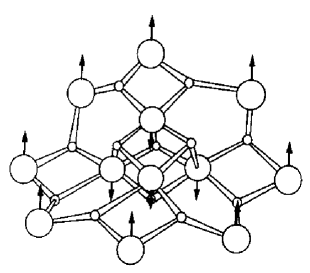
FIG. 1.: Mn₁₂-acetate molecule. The big circles denote manganese and the smaller ones oxygen ions. The arrows correspond to the orientation of the atomary spins in the $S=10$ ground state. The figure is reproduced from [10] under the copyright of EDP Sciences.

The main features of the experimental findings can be understood in terms of two competing relaxation mechanisms: quantum mechanical tunneling through and thermal activation over the anisotropy barrier. At high temperatures ($T>3{\rm K}$ or $T>6{\rm K}$, depending on the experiment [9]), the spins relax predominantly via thermal activation due to the phonons in the lattice. [10, 11, 12] In this regime, the relaxation time follows the Arrhenius law $\tau=\tau_{0}\exp(U/k_{\rm B}T)$, where $U/k_{\rm B}\approx 60{\rm K}$ denotes the barrier height and $\tau_{0}\approx 10^{-8}{\rm s}$ the inverse attempt frequency. [13] When temperature is lowered to $2{\rm K}<T<3{\rm K}$, the time required by the over-barrier relaxation increases exponentially but several of the excited states still remain thermally populated. In this regime, pairs of states on the opposite sides of the barrier can be brought to degeneracy by tuning the external magnetic field. This enhances the probability to tunnel across the barrier; the tunneling arises due to crystalline anisotropy and possible transverse magnetic field at the site of the spin. The tunneling amplitudes are the larger the closer to the top of the barrier the states are and, consequently, the thermal population of the higher states plays a key role in relaxation, cf. e.g. Refs. [10, 11, 12] and [14]. At still lower temperatures, tunneling and the relaxation becomes sensitive to fluctuations in the dipolar and hyperfine fields. [15] In this paper, we concentrate in the regime of thermally-activated tunneling.

Several authors have investigated the spin dynamics theoretically with the emphasis ranging from “minimal” models, assuming as simple a spin Hamiltonian ${\mathcal{H}}_{S}$ and a model of the surroundings as possible (in order to explain experiments, that is), [10, 11, 12, 14, 16, 17, 18] to more specific models for investigating the role of the dipolar and/or hyperfine interactions, [19, 21, 22] and combinations of these [12, 14, 16, 23]. The thermally activated relaxation has typically been studied using a master equation approach to describe the time evolution of the spin density matrix. [10, 11, 12, 14, 16, 17, 18, 24] The susceptibility, on the other hand, has only been treated within a phenomenological model. [5, 40]

The existing theories have been successfull in explaining the general features seen in experiments. However, several points call for further attention. 1) A microscopic calculation of the dynamic susceptibility is missing altogether. 2) The effect of a strong transverse magnetic field has not been thoroughly studied and, in particular, not in the context of the susceptibility. 3) Several authors including ourselves have found a series of side resonances to arise in their calculations [16, 18, 24] - the fact that these peaks are not in general (see Ref. [25] for exceptions) observed in experiments is not quite clear. In this work, we aim at elucidating these points and present calculations for the relaxation rates and susceptibility in a unified language that can be conveniently extended to systems with stronger couplings. We work with a Hamiltonian similar to, e.g., Ref. [18], cf. Eqs. (2), (3), and (4), but introduce an alternative framework to work with the density matrix. It is well known that all the resonances can be enhanced by a strong transverse magnetic field but we show that the resonances can also be reduced and even suppressed: Both the relaxation rate, see also Ref. [23], and susceptibility are found to display significant dependence on the direction of the transverse field suggesting that interference effects of a geometrical phase could be observed also in Mn₁₂ and, what is more, do so in the regime of thermally-activated tunneling.

The paper is organized as follows. Part II introduces the microscopic model used for Mn₁₂ and a discussion on the different interaction mechanisms in the system. In part III, we develop a time-dependent description of the system in terms of a real-time diagrammatic technique. This approach is then used to derive and evaluate the kinetic equation and the resulting master equation governing the spin dynamics. In part III B, we solve the kinetic equation for the field-dependent relaxation times $\tau(H)$ and the static susceptibility $\chi_{0}(H)$. The dynamic susceptibility $\chi(\omega;H)$ is calculated in part III C and a Kubo-type formula is found. Part IV displays the numerical results for both $\tau(H)$ and $\chi(\omega;H)$ accompanied with a discussion on the results and their relevance to experiments. In part V we sum up the work.

II System

The spin Hamiltonian of a single Mn₁₂ molecule can be written in the form ${\mathcal{H}}_{S}={\mathcal{H}}_{z}+{\mathcal{H}}_{\rm T}$. The first term,

$${\mathcal{H}}_{z}=-AS_{z}^{2}-BS_{z}^{4}-g\mu_{\rm B}H_{z}S_{z},$$ (2)

with $S_{z}$ being the spin component along the easy axis (here the $z$-direction), describes the part that commutes with $S_{z}$. It consists of the anisotropy terms of Eq. (1) and a Zeeman term which enables external biasing of the energies. The anisotropy constants have been experimentally estimated [26, 27] as $A/k_{\rm B}=0.52-0.56{\rm K}$ and $B/k_{\rm B}=0.0011-0.0013{\rm K}$; the g-factor is 1.9. [28] The resulting energy levels $E_{m}$ for the eigenstates of $S_{z}|m\rangle=m|m\rangle$ together with the potential barrier are shown schematically in Fig. 2.

FIG. 2.: Schematic of the energy diagram for $2S+1=21$ eigenstates of ${\mathcal{H}}_{z}$ together with the functional form of the potential barrier (solid line). The figure also shows examples of possible transition processes: spin-phonon coupling may change $m$ by $\pm 1$ or $\pm 2$, while the anisotropy term in ${\mathcal{H}}_{\rm T}$ yields tunnel couplings across the barrier – an example of a third-order (in $B_{4}$) process is depicted in the figure.

The second term in the Hamiltonian,

$${\mathcal{H}}_{\rm T}=-\frac{1}{2}B_{4}\left(S_{+}^{4}+S_{-}^{4}\right)-g\mu_{\rm B}(H_{x}S_{x}+H_{y}S_{y})$$ (3)

does not commute with $S_{z}$ and gives rise to tunneling. The $B_{4}$-term arises from crystalline anisotropy, $B_{4}=(4.3-14.4)\cdot 10^{-5}{\rm K}$ (below we use $B_{4}=8.6\cdot 10^{-5}$K, but the particular choice is unimportant for the results obtained),[26] while the second term is the Zeeman term corresponding to a transverse magnetic field $H_{\perp}=H\sin\theta$ (in spherical coordinates, $\theta$ is the polar angle away from the $z$-axis; the azimuth angle is denoted $\phi$: $H_{x}=H_{\perp}\cos\phi$ and $H_{y}=H_{\perp}\sin\phi$).

Figure 3 shows the eigenenergies of ${\mathcal{H}}_{S}$ as a function of the longitudinal magnetic field $H_{z}$. Away from the resonances, the eigenstates $|d\rangle$ resemble the states $|m\rangle$ and are also localized onto the different sides of the barrier – the linear field dependence of the eigenenergies stems from the Zeeman term in Eq. (2). Close to the resonances, ${\mathcal{H}}_{\rm T}$ couples the $|m\rangle$ states across the barrier and gives rise to avoided crossings in the energy diagram for $E_{d}$. The magnitude of these splittings directly gives the tunneling strengths. Depending on the states in question as well as on the magnitude of $B_{4}$ ($H_{\perp}=0$ for the moment), the splittings are found to vary enormously: from $10^{-10}$K for the choice $B_{4}/k_{\rm B}=4.3\cdot 10^{-5}$K and the states $m=\pm 10$ up to almost 2K for $B_{4}/k_{\rm B}=14.4\cdot 10^{-5}$K and the resonance $m=\pm 2$. This upper limit is already of the same order of magnitude as the level spacing and in fact even exceeds it rendering perturbative calculations of the tunneling couplings/strengths somewhat questionable. Therefore, even though we first formulate everything in a general form, independent of the choice of basis for the spins, we calculate the actual results working in the eigenbasis of ${\mathcal{H}}_{S}$. This choice of basis provides the additional advantage that it allows us to consider arbitrarily strong magnetic fields.

FIG. 3.: The eigenenergies of the 21 states as a function of $H_{z}$. The inset shows a blow up of the higher energies at low fields – note especially the avoided crossings of the states $m-m^{\prime}=4$ directly coupled by the $B_{4}$-term in ${\mathcal{H}}_{\rm T}$. There are similar, although smaller, splittings for the lower levels as well. The three arrows denote the effective barrier height that decreases with increasing $H_{z}$.

In absence of $H_{\perp}$, there is a selection rule to ${\mathcal{H}}_{\rm T}$: only states $m$ and $m^{\prime}$ that are a multiple of four apart are coupled. Experimental data do not lend support to such a rule, however, but rather suggest that all transitions are allowed. It turns out that already a tiny transverse field in Eq. (3) is sufficient in achieving this – such a field may arise due to dipolar and/or hyperfine interactions within the sample, see below, as well as due to uncertainity in the precise angle between the external field and the easy axis of the sample. We assume throughout the paper a small constant misalignment angle $\theta=1^{\circ}$ and $H_{\perp}=|{\it\bf H}|\cdot\sin\theta$. In places, we wish to investigate the effects of a significantly stronger transverse field and state so explicitly. The transverse field increases the tunnel splittings if $\phi$ is close to $n\pi/2$ ($n$ is an integer), i.e., along the $x$ and $y$-axes, or leads to oscillations in the splittings if $\phi$ is close to one of the directions $\pi(2n+1)/4$. Below we denote these special directions as the hard axes of the molecules. [29] The tunnel splittings are illustrated in Fig. 4 as a function of $H_{\perp}$ and for different angles $\phi$, see Ref. [30].

FIG. 4.: The tunnel splittings $\Delta_{m,-m}$ as a function of the transverse magnetic field; $H_{z}=0$. The three types of curves correspond to three different angles $\phi$: $0^{\circ}$ – dashed, $40^{\circ}$ – dotted, and $45^{\circ}$ – solid.

The usage of ${\mathcal{H}}_{S}$ of an isolated spin is based, first of all, on the assumption that the molecules indeed reside in their $S=10$ ground state. [32] This is well justified for the experimental temperatures below $3-6{\rm K}$ – the energy required to excite the system to the lowest excited state with $S=9$ is around 30K. The second assumption is the absence of interaction. In reality, the spins interact with each other via dipolar interaction, with the nuclear spins via hyperfine interaction, and with the phonons of the surrounding lattice. Experimental evidence shows that the dipolar interactions are small for $T>2-2.4{\rm K}$, [15, 33] while the hyperfine interactions produce an intrinsic broadening of the order of 10mT to the spin states. [12, 33] We neglect these for the moment and return to them in Sec. IV C.

The spin-phonon interaction is mediated by variations in the local magnetic field induced by lattice vibrations and distortions. For tetragonal symmetry, this can be generally formulated as, cf. Ref. [18],

$${\mathcal{H}}_{\rm sp} = g_{1}(\epsilon_{xx}-\epsilon_{yy})\otimes\left(S_{x}^{2}-S_{y}^{2}\right)+\frac{1}{2}g_{2}\epsilon_{xy}\otimes\left\{S_{x},S_{y}\right\}$$ (4)

$$+ \frac{1}{2}g_{3}\left(\epsilon_{xz}\otimes\left\{S_{x},S_{z}\right\}+\epsilon_{yz}\otimes\left\{S_{y},S_{z}\right\}\right)$$ (5)

$$+ \frac{1}{2}g_{4}\left(\omega_{xz}\otimes\left\{S_{x},S_{z}\right\}+\omega_{yz}\otimes\left\{S_{y},S_{z}\right\}\right)$$ (6)

where $\epsilon_{\alpha\beta}$ and $\omega_{\alpha\beta}$ are the symmetric and antisymmetric strain tensors, respectively, and $g_{i}$ ($i$=1,2,3,4) are the spin-phonon coupling constants. For these, we adopt the values from Ref. [18]: $g_{1}=g_{4}/2=A$ and $|g_{2}|\approx g_{1}$ and $|g_{3}|\approx g_{4}$. In leading order in $g_{i}$’s, ${\mathcal{H}}_{\rm sp}$ produces transitions such that for, $g_{1,2}$-terms, $\Delta m=\pm 2$ and, for $g_{3,4}$-terms, $\Delta m=\pm 1$. The phonons themselves are described by

$${\mathcal{H}}_{\rm ph}=\sum_{\vec{k}\sigma}\omega_{\vec{k}\sigma}b_{\vec{k}\sigma}^{\dagger}b_{\vec{k}\sigma}$$ (7)

as a bath of noninteracting bosons.

To be more quantitative, the phonons are assumed to be plane waves with a linear spectrum and three modes – two transverse and one longitudinal – denoted by $\sigma$. The elements of the strain tensor, $\epsilon_{\alpha\beta}\equiv(\partial_{\alpha}u_{\beta}+\partial_{\beta}u_{\alpha})/2$ and $\omega_{\alpha\beta}\equiv(\partial_{\alpha}u_{\beta}-\partial_{\beta}u_{\alpha})/2$, are defined in terms of the local displacement vector

$$u_{\alpha}(\vec{r}) = \sum_{\vec{k}\sigma}\sqrt{\frac{\hbar}{2NM\;\omega_{\vec{k}\sigma}}}\;e_{\alpha}^{(\sigma)}\;[b_{\vec{k}\sigma}^{\dagger}+b_{\vec{k}\sigma}]\;e^{i\vec{k}\cdot\vec{r}}.$$ (8)

Here $b_{\vec{k}\sigma}^{(\dagger)}$ are the bosonic operators for phonons with wave vector $\vec{k}$, $\omega_{\vec{k}\sigma}$ is the correponding frequency, and $e_{\alpha}^{(\sigma)}$ the $\alpha$th element (of $x$, $y$, and $z$) of the polarization vector; $N$ is the number of unit cells and $M$ the mass per unit cell.

Above we considered the energy scales inherent to ${\mathcal{H}}_{S}$, and the spin-phonon rates, which are found below (Apps. A and B) to be typically of the order of $10^{-5}-10^{-4}$K, fall in between the extremes of the tunnel splittings. This value is very small compared to the stronger tunneling couplings and seems to suit well for a perturbative treatment. On the other hand, for the low-lying and weakly coupled states the spin-phonon rates may be several orders of magnitude larger than the tunnel splittings and one would expect the tunneling to be suppressed. However, the intermediate regime, where the tunneling and spin-phonon rates are of the same order of magnitude, requires some extra care, see below.

III Dynamics

The magnetization measured in experiments is the molecular magnetization $M(t)$ magnified by the large number of molecules in the samples. Let us define $M(t)$ in terms of the reduced density matrix $\rho(t)={\rm Tr}_{\rm ph}[\rho^{\rm tot}(t)]$ ($\rho^{\rm tot}(t)$ is the full density matrix)

$$M(t) = g\,\mu_{\rm B}\;\langle S_{z}(t)\rangle$$ (9)

$$\equiv g\,\mu_{\rm B}\;{\rm Tr}_{S}[S_{z}\rho(t)]=g\,\mu_{\rm B}\sum_{m}m\cdot\rho_{m,m}(t)$$ (10)

The reduced density matrix $\rho(t)$ describes the spin degrees of freedom in the presence of the phonon reservoir – its diagonal elements are just the probabilities for the spin to be in the states $|m\rangle$. Our strategy is to start with the general formulation

$$\langle S_{z}(t)\rangle={\rm Tr}[S_{z}(t)\cdot\rho_{0}^{\rm tot}],$$ (11)

where $\rho_{0}^{\rm tot}=\rho^{S}\rho^{\rm ph}$ denotes the initial density matrix of the whole system encompassing the spin and phonon degrees of freedom. However, this does not contain the interaction between the two: we assume that the coupling is turned on adiabatically and only enters the time evolution of $S_{z}(t)$ (in Heisenberg picture and with the convention $\hbar=1$)

$$\langle S_{z}(t)\rangle={\rm Tr}[e^{+i\!\int_{t_{0}}^{t}\!\!dt^{\prime}{\mathcal{H}}(t^{\prime})}S_{z}\;e^{-i\!\int_{t_{0}}^{t}\!\!dt^{\prime}{\mathcal{H}}(t^{\prime})}\cdot\rho_{0}^{\rm tot}].$$ (12)

In order to evaluate Eq. (12) and to describe the dynamics of the system more quantitatively, we introduce a real-time diagrammatic language that is applicable to any mesoscopic system comprising a part with a finite number of states linearly coupled to an external heat (or particle) reservoir. [35]

A Diagrammatic language

Equation (12) can be written as a diagram depicted in Fig. 5. In this equation, the spin-phonon interaction terms can be separated from the noninteracting part of the Hamiltonian by shifting to the interaction picture with respect to ${\mathcal{H}}_{0}={\mathcal{H}_{S}}+{\mathcal{H}}_{\rm ph}$ (indicated with the subscript I)

$$\langle S_{z}(t)\rangle = {\rm Tr}[\rho_{0}^{\rm tot}\cdot S_{z}(t)]$$ (13)

$$= {\rm Tr}[\rho_{0}^{\rm tot}\cdot\tilde{T}e^{+i\!\int_{t_{0}}^{t}\!\!dt^{\prime}{\mathcal{H}}_{\rm sp}(t^{\prime})_{\rm I}}S_{z}(t)_{\rm I}\;Te^{-i\!\int_{t_{0}}^{t}\!\!dt^{\prime}{\mathcal{H}}_{\rm sp}(t^{\prime})_{\rm I}}]$$ (14)

where ($\tilde{T}$) $T$ is the (anti-)time-ordering operator and $\rho_{0}^{\rm tot}$ has been moved to the front (this is allowed by the invariance of trace under a cyclical permutation of its arguments).

FIG. 5.: Diagrammatic representation of Eq. (12), reading the expression from right to left and starting at time $t_{0}$ at the initial state described by $\rho_{0}^{\rm tot}$, then propagating forward (upper propagator) in time to time $t$, where $S_{z}$ (vertex) is to be evaluated, and returning backwards (lower propagator) in time to $t_{0}$. In such diagrams, the trace is always implicitly assumed.

We proceed by eliminating the phonon degrees of freedom with the aim to obtain an effective theory for the dynamics of the spin system. We first separate the trace and introduce time-ordering $T_{\rm K}$ along the closed Keldysh-contour in Fig. 5

$${\rm Tr}[\rho_{0}^{\rm tot}\!\! \!\cdot\! \!\!S_{z}(t)]=$$ (15)

$$= {\rm Tr}_{S}\{\rho_{0}^{S}\;{\rm Tr_{ph}}\rho_{0}^{\rm ph}\;T_{\rm K}e^{-i\int_{\rm K}dt^{\prime}{\mathcal{H}}_{\rm sp}(t^{\prime})_{\rm I}}S_{z}(t)_{\rm I}\}.$$ (16)

The exponential, expanded in powers of ${\mathcal{H}}_{\rm sp}$, reads

$$T_{\rm K}e^{-i\int_{\rm K}dt^{\prime}{\mathcal{H}}_{\rm sp}(t^{\prime})_{\rm I}}=\sum_{m=0}^{\infty}(-i)^{m}$$ (17)

$$\;\;\cdot\!\int_{\rm K}\!dt_{1}\!\int_{\rm K}\!dt_{2}...\!\int_{\rm K}\!dt_{m}T_{\rm K}\{{\mathcal{H}}_{\rm sp}(t_{1})_{\rm I}\;{\mathcal{H}}_{\rm sp}(t_{2})_{\rm I}\;...\;{\mathcal{H}}_{\rm sp}(t_{m})_{\rm I}\}$$ (18)

with $t_{1}>t_{2}>...>t_{m}$. Each ${\mathcal{H}}_{\rm sp}(t_{i})_{\rm I}$ is represented as a vertex on the Keldysh contour. In the next step, this expansion together with the explicit expression (4) for ${\mathcal{H}}_{\rm sp}$ is inserted into Eq. (16) and the trace over the phonons is performed by using Wick’s theorem. As a consequence, the phonon operators are pairwise contracted: ${\rm Tr}_{\rm ph}\rho_{0}^{\rm ph}b^{\dagger}(t)b(t^{\prime})=\langle b^{\dagger}(t)b(t^{\prime})\rangle$ and ${\rm Tr}_{\rm ph}\rho_{0}^{\rm ph}b(t)b^{\dagger}(t^{\prime})=\langle b(t)b^{\dagger}(t^{\prime})\rangle$. Here, the phonons are considered as a reservoir that is not perturbed by the single spin – the bath remains in equilibrium and the contractions are given by the Bose-Einstein distribution $\langle b_{\vec{k}\sigma}^{\dagger}b_{\vec{k}\sigma}\rangle=[\exp(\beta\omega_{\vec{k}\sigma})-1]^{-1}$. In terms of the diagrams this means that the vertices get coupled (in all possible ways) by interaction or phonon lines which correspond to just these contractions, cf. Fig. 6. The general rules for evaluating the diagrams are given in App. A and the contributions from the interaction lines are calculated in App. B.

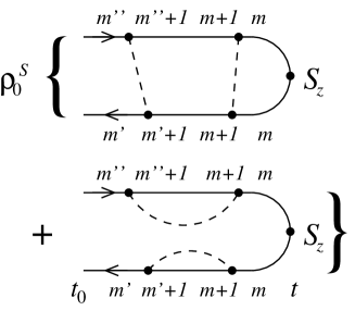
FIG. 6.: Examples of the diagrams arising after integration over phonons. The indices on the forward (backward) propagators correspond to the spin states and, in particular, the first (second) index of $\rho(t)$. Note that in general $m$, $m^{\prime}$, and $m^{\prime\prime}$ may all be unequal if tunneling is allowed along the propagator and if we also consider the nondiagonal elements of $\rho(t)$.

All the diagrams, e.g., those in Fig. 6, are composed of two kinds of elements that can be distinguished by drawing a vertical line through the diagram and checking whether it cuts phonon lines or not. If it does not, the corresponding part of the diagram represents free evolution of the spin; if it does, the part of the diagram between successive periods of free evolution corresponds to spin-phonon interaction and, more particularly, to a transition rate between different spin states. The sum of all the possible diagrams with the interaction lines is denoted as $\Sigma$ and, when evaluated, its terms are $O(g^{2n})$ where $g$ is the spin-phonon coupling constant and $n$ the number of interaction lines in the diagram, cf. Appendices A and B, and below. The full time evolution of $\langle S_{z}(t)\rangle$ can be expressed as in Fig. 7a in terms of the two kinds of contributions, just discussed. In lowest order in $g$, $\Sigma$ is given by the diagrams shown in part (b) of the figure.

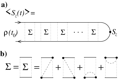
FIG. 7.: Diagrammatic expression for (a) the expectation value of $S_{z}$ in terms of the element $\Sigma$, which corresponds to the phonon-induced transition rate of the spin. (b) Diagrammatic representation for $\Sigma$ in $O(g^{2})$.

B Kinetic equation

The reduced density matrix defined as

$$\rho_{m,m^{\prime}}(t)\equiv\big{\langle}(|m^{\prime}\rangle\langle m|)(t)\big{\rangle}$$ (19)

accounts for the full time evolution of the spin in the presence of the spin-phonon interaction. Its diagrammatic expansion is analog to Fig. 7a with $S_{z}$ being replaced by $|m^{\prime}\rangle\langle m|$. Setting $t_{0}=0$ and differentiating with respect to time, we obtain the kinetic equation

$$\dot{\rho}(t)+i[{\mathcal{H}}_{S},\rho(t)]=\int_{0}^{t}dt^{\prime}\Sigma(t,t^{\prime})\rho(t^{\prime})$$ (20)

The commutator on the l.h.s. of Eq. (20) corresponds to the free (Hamiltonian) time evolution of the spin, while the integral on the r.h.s. describes a dissipative interaction which is nonlocal in time and contains the spin-phonon coupling terms.

The time dependence of the kernel $\Sigma(t,t^{\prime})=\Sigma(t-t^{\prime})$ is evaluated explicitly in Apps. A and B up to order $O(g^{2})$, compare Fig. 7b. It depends only on the time difference since the Hamiltonian is time-translationally invariant. According to Eq. (A8), we find that $\Sigma(t-t^{\prime})$ is a fast decaying function of time, and we make the simplifying Markov assumption that $\rho(t)$ remains essentially constant over the time period $\Delta t$ within which $\Sigma(t-t^{\prime})$ decays to zero and take $\rho(t)$ in front of the integral. [36] This is justified at least for the longest relaxation time $\tau_{1}$ (see below). For convenience, we also take the upper integration limit to infinity.

After taking $\rho(t)$ out of the integral in Eq. (20) the integration over time (up to infinity) can be performed and we are left with a constant $\Sigma$. This is evaluated in App. B and corresponds to the diagrams in Figs. 7b and 21a and b, see also below. The kinetic equation (20) becomes

$$\dot{\rho}(t)=-iL_{0}\,\rho(t)+\Sigma\,\rho(t)\equiv W\rho(t)$$ (21)

with $L_{0}\equiv[{\mathcal{H}}_{S},.]$. This is similar to the master equation formulations in the literature [12, 14, 16, 17, 18] and may be solved for the eigensolutions of $W$

$$\dot{\rho}^{(i)}(t) = W\rho^{(i)}(t)=\lambda_{i}\rho^{(i)}(t)$$ (22)

$$\rho^{(i)}(t) = \rho^{(i)}(0)\cdot e^{\lambda_{i}t}.$$ (23)

The real parts of the eigenvalues correspond to relaxation rates $Re(\lambda_{i})=-\tau_{i}^{-1}$.

The eigensolution of $W$ with $\lambda_{0}=0$ corresponds to the stationary state, defined as $\dot{\rho}^{(0)}(t)=0$ with $\rho^{(0)}(t)=\rho^{(0)}$. The diagonal elements of $\rho$ are the thermal probabilities to find the spin in the respective states. In the $m$-basis, the static magnetization and susceptibility are readily expressed in terms of the diagonal components $\rho_{m}^{(0)}=\rho_{m,m}^{(0)}$ yielding

$$M_{0}=g\mu_{\rm B}\sum_{m}m\,\rho_{m}^{(0)}\!\!\!\!\!\!\!\!\!\!\!\!\!\!\!\!\!\!\!\!\!\!\!$$ (24)

$$\chi_{0}=\frac{\partial M_{0}}{\partial H_{z}} = g\mu_{\rm B}\sum_{m}m\cdot\frac{\partial\rho_{m}^{(0)}}{\partial H_{z}}.$$ (25)

Since the stationary probabilities are given by Boltzmann factors we obtain in the absence of tunneling

$$\chi_{0}=-\frac{(g\mu_{\rm B})^{2}}{k_{\rm B}T}\sum_{m,m^{\prime}}m(m^{\prime}-m)\rho_{m}^{(0)}\rho_{m^{\prime}}^{(0)}.$$ (26)

In the precence of tunneling, this form remains essentially the same up to transverse fields of the order of $1{\rm T}$ (in this range most of the tunneling splittings are too small compared to the level spacing in order to change the result considerably).

For all the other solutions $Re(\lambda_{i})<0$ and the vectors $\rho^{(i)}(t)$ correspond to deviations from $\rho^{(0)}$. The longest relaxation time $\tau_{1}$ is several orders of magnitude larger than $\tau_{2}$ and the respective solution is interpreted to correspond to the over-barrier relaxation.

Above we have considered the full (reduced) density matrix $\rho(t)$. In appendix C, we discuss the choice of the basis and argue that the $d$-basis has certain advantages and, e.g., in the case of strong tunneling compard to the spin-phonon rates, it allows the restriction to the diagonal elements of $\rho(t)_{d,d^{\prime}}$ only. The nondiagonal elements become important when the rates for the tunneling and the spin-phonon coupling are of the same order of magnitude.

C Ac-susceptibility

In this section we derive an expression for the dynamic susceptibility

$$\chi(\omega) \equiv \int_{0}^{\infty}d\tau e^{i\omega\tau}\chi(\tau)$$ (27)

$$\chi(t-t^{\prime}) = \frac{\partial\!\acute{}\;M(t)}{\partial\!\acute{}\;H_{z}(t^{\prime})}=g\,\mu_{\rm B}\frac{\partial\!\acute{}\;\langle S_{z}(t)\rangle}{\partial\!\acute{}\;H_{z}(t^{\prime})}$$ (28)

starting from the Hamiltonian ${\mathcal{H}}$ and formulating the expectation value in Eq. (28) in terms of diagrams. For convenience, we assume in the following that $H_{\perp}$ can be tuned to any (static) value independent of $H_{z}$ and that the actual measurement is done by applying a tiny ac-excitation field $h_{z}(\omega)$ on top of the static $H_{z}$. The more general calculation of $\partial\!\acute{}\;M_{\alpha}(t)/\partial\!\acute{}\;H_{\beta}(t^{\prime})$, $\alpha,\beta=x,y,z$, can be carried out along the same lines.

The derivation with respect to $H_{z}(t^{\prime})$ acts on the terms $\exp[\mp i\int\!dt^{\prime}{\mathcal{H}}_{z}(t^{\prime})]\propto\exp[\mp i(-g\,\mu_{\rm B})\int\!dt^{\prime}S_{z}(t^{\prime})H_{z}(t^{\prime}))]$ in Eq. (12) and may occur on either the forward or backward propagator of the diagrams (minus and plus signs, respectively). The derivation takes down a factor $\pm ig\mu_{\rm B}S_{z}(t^{\prime})$ and we obtain

$$\chi(t-t^{\prime})=i(g\mu_{\rm B})^{2}\langle[S_{z}(t),S_{z}(t^{\prime})]\rangle$$ (29)

which, when inserted to Eq. (27), is just the Kubo formula for the linear response to an external magnetic field.

Susceptibility can be expressed diagrammatically starting from either of the equations (28) or (29). In either case, $S_{z}(t)$ is written at the latest point to the right. For Eq. (28), $\partial\!\acute{}\;/\partial\!\acute{}\;H_{z}(t^{\prime})$ may act on either of the propagators, while, for Eq. (29), the terms of the commutator are ordered on the contour reading them from right (earlier) to left (later times). It is the most convenient to work in the eigenbasis where it is sufficient to consider the diagonal elements only, see App. C. In this case, if $S_{z}(t^{\prime})$ falls in between $\Sigma$’s in the diagram in Fig. 7a, the commutator equals zero – we only need to be concerned with the $\Sigma$ parts.

Let us set $t_{0}=0$ and define $\tilde{\Sigma}(t^{\prime\prime},0)$ as in Fig. 7b but with $S_{z}(t^{\prime})$ ($0<t^{\prime}<t^{\prime\prime}$) inserted onto one of the propagators. Furthermore, let us assign the part $e^{i\omega(t^{\prime\prime}-t^{\prime})}$ of the Laplace transform to the definition of $\tilde{\Sigma}(t^{\prime\prime},0)$. This is then the part of the integrand in Eq. (27) appearing between times $t=0$ and $t=t^{\prime\prime}$. On the forward propagator, this yields a factor $ig\mu_{\rm B}m_{d,d^{\prime}}\equiv ig\mu_{\rm B}\langle d^{\prime}|S_{z}|d\rangle$ when acting on the state $d$ on the propagator and changing this to the state $d^{\prime}$ ($d$-basis is not the eigenbasis of $S_{z}$). On the backward propagator, there is a further minus sign. As to the whole diagram, see Fig. 8, the system is in the stationary state before $t_{0}=0$, described by $\rho^{(0)}$ – this corresponds to the requirement that the expectation value $\langle S_{z}\rangle$ is taken with respect to the stationary state. [One could extend the definition of the susceptibility to account for experiments with an additional time-dependent (e.g. constantly sweeped) magnetic field $H_{z}(t)$ and consider initial states before $t^{\prime}$ that are combinations of the stationary and the relaxing modes.] After $\tilde{\Sigma}(t^{\prime\prime},0)$, there may be any number of $\Sigma$’s between this and the final time $t$ – the sum of such series is denoted $\Pi(t,t^{\prime\prime})$. Finally the resulting diagram/expression is Laplace transformed – $e^{i\omega(t-t^{\prime})}$ being divided into two parts, one denoted by the dashed line running through the diagram from time $t^{\prime\prime}$ to $t$ and the other one extending from $t^{\prime}$ to $t^{\prime\prime}$ and already belonging to the above definition of $\tilde{\Sigma}$.

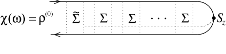
FIG. 8.: Diagrammatic representation of $\chi(\omega)$, see text for details.

In evaluating the diagram in Fig. 8, we vary $t^{\prime}$ within $\tilde{\Sigma}(t^{\prime\prime},0)$, and extend the integrations of $t$ and $t^{\prime\prime}$ to infinity. This yields

$$\int_{t^{\prime}}^{\infty}dte^{i\omega(t-t^{\prime})}\langle[S_{z}(t),S_{z}(t^{\prime})]\rangle=\sum_{d,d^{\prime},d^{\prime\prime}}m_{d}$$ (30)

$$\int_{0}^{\infty}\!\!\!dt^{\prime\prime}\int_{t^{\prime\prime}}^{\infty}\!\!\!dt\int_{0}^{t^{\prime\prime}}\!\!\!dt^{\prime}\Pi(t,t^{\prime\prime})_{d,d^{\prime\prime}}\tilde{\Sigma}(t^{\prime\prime},0)_{d^{\prime\prime},d^{\prime}}\rho_{d^{\prime}}^{(0)}e^{i\omega(t-t^{\prime\prime})},$$ (31)

where, for brevity, we denote the diagonal states by just one index $d$, e.g., $m_{d}=m_{d,d}$, see above. The integrations can be carried out one by one in the order $t^{\prime}$, $t$ (which yields $\Pi(z=\omega)$), and $t^{\prime\prime}$ to yield

$$\chi(\omega)=-(g\mu_{\rm B})^{2}$$ (32)

$$\;\;\;\;\;\;\;\sum_{d,d^{\prime},d^{\prime\prime}}\,m_{d}\left[\frac{1}{-i\omega+iL_{0}-\Sigma(\omega)}\right]_{d,d^{\prime\prime}}\tilde{\Sigma}(\omega)_{d^{\prime\prime},d^{\prime}}\rho^{(0)}_{d^{\prime}},$$ (33)

where $\Sigma(\omega)$ is defined as the Laplace transform of $\Sigma(t,0)$. The explicit expressions for $\tilde{\Sigma}(\omega)_{d,d^{\prime\prime}}$ turn out lengthy and are omitted here.

The resolvent in Eq. (32) is treated in terms of the eigensolutions of $W\rho(t)$ and the appropriate projections of the terms $\tilde{\Sigma}(\omega)\rho^{(0)}=\sum_{i}c_{i}\rho^{(i)}$ are used. In particular, for the component along the relaxing mode $\rho^{(1)}(t)$, the resolvent in Eq. (32) reads

$$\frac{1}{-i\omega+iL_{0}-\Sigma(\omega)}=\frac{1}{-i\omega-W(\omega)}\approx\frac{1}{-i\omega+\tau_{1}^{-1}}.$$ (34)

The approximate sign is due to the Markov approximation where $\Sigma(\omega)\approx\Sigma(0)$, cf. App. D. Apart from one $\tau_{1}$ this is the well-known factor in expressions for susceptibility, see e.g. Refs. [39] or [40]. The rest of Eq. (32) reduces to a prefactor roughly proportional to $\tau_{1}^{-1}$ but with weak $H_{z}$ and $\omega$-dependences. For the low frequency limit, we recover the static susceptibility, i.e., $\lim_{\omega\rightarrow 0}\chi(\omega)=\chi_{0}$ where $\chi$ is given by Eq. (26).

IV Results

In this section, we concentrate on results obtained in the eigenbasis of ${\mathcal{H}}_{S}$. This choice is advocated by three points. First, it allows us to consider much stronger transverse fields (see the discussion on energy scales in Part II) than the common approach to calculate tunnel splittings in the leading-order perturbation theory; [34, 14] second, the origin of the Lorentzian shape of the resonances is seen to arise naturally from the tunnel splittings. [16, 24] The third point is that, in this basis, all the relevant properties of the system are captured by the diagonal elements $\rho(t)_{d,d}$ only. [38] This feature also improves the performance of the numerics. We also present results obtained with the full $\rho(t)$ and discuss the differences as examples of phonon-induced decoherence. The energies are expressed in kelvin, magnetic fields in teslas, and rates in $s^{-1}$.

A Relaxation rates

The relaxation rate as a function of the longitudinal magnetic field $H_{z}$ is shown in Fig. 9. The overall behaviour is of the Arrhenius form, i.e., $\tau\approx\tau_{0}\exp[\beta U(H_{z})]$ where $\tau_{0}$ only gives a constant offset to the semilogarithmic figure and $U$ is the effective height of the barrier, see Fig. 3. On top of this exponential field dependence, there are series of resonances located at

$$H_{z}^{m,m^{\prime}}=-\frac{m+m^{\prime}}{g\mu_{\rm B}}\left[A+B(m^{2}+{m^{\prime}}^{2})\right]$$ (35)

corresponding to the values of the external field that brings the states $m$ and $m^{\prime}$ on-resonance; the resonances form groups close to the fields $H_{z}\approx nH_{1}$ where $n=m+m^{\prime}$ and $H_{1}=\frac{A}{g\mu_{\rm B}}$, see Fig. 9. The broadest of the resonances resemble those seen in usual experiments, while most of the resonances are too narrow to be seen and, as is discussed below, already the phonon coupling is sufficient to suppress them. One of the main topics of this paper is the possibility to detect some of the satellite peaks by the application of a relatively strong transverse field $H_{\perp}$ as well as to suppress the already visible peaks by pointing $H_{\perp}$ along one of the hard axes.

FIG. 9.: Relaxation rate $\Gamma=1/\tau$ as a function of the longitudinal magnetic field: without tunneling (dashed) and with tunneling (solid). Here, only the diagonal density matrix elements are used. The large offset between the two curves is due to the broad Lorentzian shapes under the even resonances: there is a strong direct coupling between the states $m=-m^{\prime}=-2$ around $H_{z}=0$, $m=-3,m^{\prime}=1$ under the second series of peaks ($H_{z}\approx 2H_{1}$), and $m=-4,m^{\prime}=0$ under the fourth series of peaks ($H_{z}\approx 4H_{1}$). The sharp resonances arise due to tunnel coupling of lower-lying states $m$; their height reflects the energies $E_{m}$ via the Arrhenius law $\Gamma\propto\exp[-\beta(E_{m}-E_{-10}])$, and the peak width is given by the tunnel splitting. Here the temperature is 2.5K.

The whole curve in Fig. 9 can be understood in terms of the expression

$$\tau=\sum_{n}\tau_{0}^{(n)}D_{n}(H_{z})e^{\beta U_{n}(H_{z})}$$ (36)

where the index $n$ enumerates the resonances (pairs of states $m_{n}$ and $m_{n}^{\prime}$). As discussed in App. E, there is a certain $\tau_{0}^{(n)}$ for each resonance; the function $D_{n}(H_{z})$ is a tunneling-induced Lorentzian that yields the peak shapes, and $U_{n}(H_{z})$ is the effective barrier height for the $n$th resonance, i.e., $U_{n}=E_{m_{n}}-E_{-10}$ ($E_{-10}$ is the energy of the metastable minimum). The widths of the Lorentzian peaks are given by

$$\delta H_{z}=\frac{4|\Delta_{n}|}{g\mu_{\rm B}|m_{n}-m_{n}^{\prime}|},$$ (37)

where $2|\Delta_{n}|$ is the tunnel splitting between the resonant states, cf. App. E. As is seen in the figure and also suggested by the inset in Fig. 3, the background is not given by the over-barrier relaxation but by the “leakage” due to the direct coupling of states with $m-m^{\prime}=\pm 4$, e.g., $m=\pm 2,m^{\prime}=\mp 2$ close to $H_{z}=0$ and $m=\pm 1,m^{\prime}=\mp 3$ close to $H_{z}=2H_{1}$. This effectively lowers the barrier height to $U\approx E_{-2}-E_{-10}$. The rates that determine $\tau_{0}^{(n)}$, depend only weakly on temperature, the resonant states, and $H_{z}$, cf. App. E. This is in line with the experimental observation that the estimated prefactor of the Arrhenius law, $\tau_{0}$, varies within an order of magnitude for different samples and resonances.

The sharpness of the narrowest peaks in Fig. 9 is an artefact of the reduced model used so far, i.e., neglect of the nondiagonal matrix elements, and let us next consider two things affecting these peaks: decoherence due to spin-phonon coupling and the broadening effect of a transversal magnetic field $H_{\perp}$. For other contributions such as the hyperfine and dipolar interactions, see Sec. IV C.

The decay of the nondiagonal elements of the density matrix is a classical definition of decoherence and this is also what is seen here when the above calculation is performed using the full $\rho(t)$. Inclusion of the off-diagonal elements still produces Lorentzian peaks but now the narrow resonances – with widths of the same order of magnitude as the spin-phonon coupling – are broadened and reduced in height. The narrowest peaks may even be completely suppressed, see the solid-line curves in Fig. 10. Despite its intuitive appeal, the suppression of the narrow peaks should be taken only qualitatively because of the limitations of the Born approximation used in treating the spin-phonon coupling. For this reason, the following considerations are restricted to regimes where the effect of the nondiagonal elements of $\rho(t)$ is negligible.

FIG. 10.: Magnification of the first and second clusters of peaks of Fig. 9 magnified (solid line). The different curves correspond to: $H_{\perp}=0.0$T (solid), 0.01T (dotted), 0.05T (dashed), 0.1T (long dashed), and 0.2T (dot dashed); $\phi=0^{\circ}$ for all the curves. The peaks further to the right correspond to resonances between lower states, hence the higher maxima. The peaks (from left to right) correspond to the resonances $m=1,..,4,m^{\prime}=-m-1$ in the left figure (the two first ones are merged together) and $m=2,..,5,m^{\prime}=-m-2$ in the right figure. Here we used also the offdiagonal elements of $\rho(t)$ with the result that some of the sharper peaks are reduced in height or even suppressed due to spin-phonon coupling. The peak widths show strong $H_{\perp}$-dependence except for the second and fourth peaks on the right – these arise from $B_{4}^{2}$ and $B_{4}^{3}$-type of coupling. Once the peak widths due to the tunnel splittings exceed the phonon-induced width, the peak heights are essentially determined by the energy $U_{n}=E_{n}-E_{-10}$ needed to reach the resonant states.

The suppressing effect of the spin-phonon coupling being essentially a constant, the sharper resonances can be made observable by broadening them with a transverse field $H_{\perp}$; even ground state tunneling has been observed in high enough fields. [42] The various tunnel splittings are shown in Fig. 4 as a function of $H_{\perp}$ pointed to three different directions $\phi$. It can be seen that for small values of the field, the splittings are essentially independent of the chosen angle, see also Fig. 11. Furthermore, tunnel splittings between states that can be coupled with sole $B_{4}$ terms of ${\mathcal{H}}_{\rm T}$ are quite insensitive to the transverse field below 0.1-0.2T. Figure 10 illustrates the effect of $H_{\perp}=H_{x}$ onto the two first series of peaks increasing $H_{x}$ monotonously increases the tunnel splittings. The resonances that initially ($H_{x}=0$) were broader than ${\tau_{0}^{(n)}}^{-1}$ are seen to retain their height; the narrower peaks, such as the two shown in the insets, are strongly broadened with increasing $H_{x}$ and also their heights increase once their widths become larger than the spin-phonon rates.

A transverse field cannot only increase the tunnel splittings but it can also reduce them, see Fig. 4. In the ideal case, the splittings can even be suppressed by varying the angle $\phi$ where the transverse field is pointed. For the zeroth peak, i.e., for $H_{z}\approx 0T$, all ten resonances occur at the same position and the suppression of any one of them is obscured in the relaxation rate curves by the simultaneous broadening of other resonances. For this reason, let us first focus on the resonances occuring at finite $H_{z}$ and return to the $H_{z}\approx 0$ case in the next section.

Figure 11 shows the tunnel splittings $\Delta_{4,-5}$ and $\Delta_{3,-5}$, respectively, as a function of $H_{\perp}$ and for four different values of $\phi$. The former corresponds to the resonance shown in the left inset of Fig. 10, while the latter corresponds to the broad resonance in the right panel of Fig. 10 which is also the one seen in experiments at $H_{z}\approx 2H_{1}$. Figure 11 also exemplifies some general properties of the tunnel splittings. As already mentioned above, the $\Delta$’s depend only weakly on $\phi$ for low $H_{\perp}$, while for larger fields and $\phi$ close to the hard axes, the tunneling amplitudes are successively increased and reduced as $H_{\perp}$ is increased. On the other hand, with $H_{\perp}$ held fixed to one of the suppression points, the $\Delta$’s oscillate as a function of $\phi$. Similar to recent work on Fe₈, see e.g. Ref. [44], these phenomena are attributed to alternating constructive and destructive interference of the geometrical phase in the tunneling amplitudes. [45, 46] The number of minima for a given $\Delta_{m,m^{\prime}}$ appears to be, as was also pointed out in Ref. [23], given by the number of $B_{4}$-terms involved in coupling the states $m$ and $m^{\prime}$. This ranges from zero at the top of the barrier to five for the gound states $m=\pm 10$, cf. Fig. 4.

FIG. 11.: The tunnel splittings $\Delta_{4,-5}$ (left) and $\Delta_{3,-5}$ (right) as a function of the transverse magnetic field when $H_{z}$ is kept fixed at the position of the corresponding resonance, 0.4581T and 0.9045T, respectively. In both figures, the four curves correspond to different angles $\phi$: $0^{\circ}$ – dot-dashed, $40^{\circ}$ – dotted, $43^{\circ}$ – dasheded, and $45^{\circ}$ – solid; the vertical axes are the same.

Figure 12 shows the relaxation rates corresponding to the resonances of Fig. 11 with $H_{\perp}$’s chosen to match the first points of suppression $H_{\perp}^{m,m^{\prime}}$. The resonance width is found to be very sensitive to $\phi$ quite as expected and, for $\phi=45^{\circ}$, the left-most peak becomes suppressed. Note, that the suppression is also quite sensitive to the value of $H_{\perp}$ as well and the higher peaks in Fig. 12 are hardly affected at all by changes in $\phi$.

FIG. 12.: Relaxation rate $\tau^{-1}$ as in Fig. 10 but now for stronger transverse field $H_{\perp}$ and for different angles $\phi$. The line types and angles are as in Fig. 11 and the values of $H_{\perp}=0.4311$T and 0.2643T are chosen to match the first suppression points (for the actual suppression occurring at the minimum value for $\Delta$ the values for $H_{\perp}$ should be given with even higher accuracy). Temperature is 2.5K.

B Ac-susceptibility

In explaining experimental results, the susceptibility $\chi(\omega)$ is often described by the formula

$$\chi(H,T,\phi,\theta,\omega)=\frac{\chi_{0}(H,T,\theta)}{1-i\omega\tau(H,T,\phi,\theta)}$$ (38)

(39)

where $\tau(H,T,\phi,\theta)$ is the relaxation time, $\omega$ the frequency of the small excitation field, and $\chi_{0}(H,T,\theta)$ the static susceptibility, cf. Ref. [5]. We emphasize here the $\phi$-dependence as we wish to investigate the interference effects and resulting oscillations in $\tau_{1}$ (below we do not explicitly write the parametric dependences of $\tau$ but they are implicitly assumed). Equation (39) relates to the results of Sec. III C as follows. Equation (32) formally accounts for all the modes $i$ and for each mode divides into two contributions, one being $1/(1-i\omega\tau_{i})$ and the other the respective prefactor. It turns out that, for most parameter values, the over-barrier relaxation, i.e., the mode $i=1$ strongly dominates over the others and one can use Eq. (39) to a good approximation. Figure 13 illustrates the two contributions to Eq. (39); they form the basis for understanding the following results. In all figures, the susceptibility is expressed for a single spin and in units of ${\rm KT}^{-2}$.

In the present model, the main correction to Eq. (39) corresponds to an intra-valley mode describing transitions between the two lowest states on the same side of the anisotropy barrier. This correction increases with increasing $H_{z}$ and temperature and, for the parameters and the curves of $\chi_{0}$ in Fig. 13, becomes of the same order of magnitude as the actual relaxing mode once $H_{z}\approx 0.9-1$T. However, such a mode corresponds to very high frequencies and is neglected below. There could be also other sources of high-frequency contributions such as dipole-dipole flip-flops, nuclear spin dynamics, or moving impurities but these are beyond the scope of this work.

FIG. 13.: Static susceptibility $\chi_{0}$ as a function of the longitudinal magnetic field shown for different temperatures: 2K (solid), 2.5K (dotted), 3K (dashed), 4K (long dashed), and 5K (dot-dashed). The dynamic susceptibility $\chi(\omega)$ is essentially composed of $\chi_{0}$ multiplied by the real and imaginary parts of $1/(1-i\omega\tau)$ shown in the inset as the solid and dashed lines, respectively.

As to the actual results, it is in principle sufficient to combine the curves for $\tau$ of the previous section with those shown in Fig. 13. The shapes of the real and imaginary parts of $1/(1-i\omega\tau)$ readily imply how the resulting susceptibility behaves if one fixes $\omega$ – it turns out that all the structure found in $\tau^{-1}$ in the previous section can also be found in $\chi(\omega)$. First, the response is the most sensitive to changes in $\tau$ when $\omega\approx\tau^{-1}$ or $\omega\tau\approx 1$, cf. the inset of Fig. 13. Second, ${\rm Re}(\chi(H_{z};\omega))$ replicates the shape of $\tau(H_{z})$ and exhibits peaks and valleys as $\tau^{-1}$ increases and decreases. This is the case with the imaginary part, ${\rm Im}(\chi(H_{z};\omega))$, as well, but only as long as $\omega\tau\geq 1$, i.e., as long as we remain on the right hand side of the peak in ${\rm Im}(\chi(H_{z};\omega))$. For lower $\omega$, $\omega\tau$ can cross the maximum point and the picture with the peaks and valleys turns upside down. These points are illustrated in Fig. 14 for a case corresponding to one of the curves in 12.

FIG. 14.: The real and imaginary parts of susceptibility for the same parameters as the dotted curves in the left panels of Fig. 12, i.e., $H_{\perp}=0.4311$T, $\phi=40^{\circ}$, and $k_{\rm B}T=2.5$K. The curves correspond to frequencies $\omega_{1}=0.02$Hz – $\chi^{\prime}$ (dotted), $\chi^{\prime\prime}$ (dashed) – and $\omega_{2}=0.5$Hz – $\chi^{\prime}$ (dot-dashed), $\chi^{\prime\prime}$ (solid). The frequencies were chosen such that $\omega_{1}<\tau^{-1}$ for the both of the peaks in Fig. 12 – hence the notches in $\chi^{\prime\prime}$, while $\omega_{2}>\tau^{-1}$ for all $H_{z}$.

Let us next consider a different scheme, keeping $H_{z}$ and $\phi$ fixed and varying $H_{\perp}$ starting from zero field. The case $H_{z}\approx 0$T is of particular interest because it allows comparison to recent experiments by Wernsdorfer done on the related material Fe₈, cf. Ref. [47] – the experimental data showed clear oscillations of the relaxation rates as a function of $H_{\perp}$ in the thermally activated regime. By choosing parameters in the feasible range of these experiments, we find somewhat similar oscillations also for Mn₁₂. Figure 15 shows first the relaxation rates for two different combinations of temperature and the longitudinal field: $T=3.0$K and $H_{z}=0.2$mT to show the behaviour close to (or at) the peak maximum and at a lower temperature, and $T=5.0$K and $H_{z}=10$mT as an example of the behaviour further away from the maximum and at a higher temperature. Also the $\phi$ dependence is shown. We would like to stress the novelty of this result: such oscillations have neither been observed nor predicted before.

FIG. 15.: Oscillations in the relaxation rate as a function of $H_{\perp}$. The lower and upper groups of curves correspond to $H_{z}=0.0002{\rm T},k_{\rm B}T=3.0{\rm K}$ and $H_{z}=0.01{\rm T},k_{\rm B}T=5.0{\rm K}$, respectively. The individual curves correspond to different angles $\phi$: $0^{\circ}$ (dashed and dot-dashed), $43^{\circ}$ (dotted), and $45^{\circ}$ (solid and long dashed).

For $\phi=0^{\circ}$, the gentle oscillations resembling a strongly-smeared staircase stem from the fact that the lower (in terms of energy; higher in terms of rates) resonances are broadened and one by one start to dominate the relaxation, see the dot-dashed curves in Fig. 16 for the tunnel splittings and Fig. 17 for the general idea. All the additional structure, seen for $\phi=45^{\circ}$, is due to the oscillations in the tunnel splittings and the suppression of some of the resonances. The positions of the notches can be compared with the structure of $\Delta_{m,-m}$ in Fig. 16 and one finds that for smaller $H_{z}$ the relaxation takes place via the lower-lying resonances such as $m=\pm 6$ and $m=\pm 7$; further away from the maximum, the broader resonances between states $m=\pm 4$ and $m=\pm 5$ act as the dominant relaxation paths.

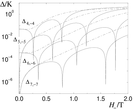
FIG. 16.: Tunnel splittings $\Delta_{m,-m}$ for four resonances relevant for Fig. 15. The dot-dashed and solid lines denote the angles $\phi=0^{\circ}$ and $45^{\circ}$, respectively.

FIG. 17.: Log-log scale schematic of Lorentzian curves on top of each other similar to the $H_{z}\approx 0$T situation for Mn₁₂. The higher the curves are the narrower they get and, on the other hand, the higher the $H_{z}$ the lower the observed resonances are. The relaxation rate is determined by the fastest possible rate, depicted in the figure with the thick solid line.

Figures 18 and 19 show the real part of the susceptibility $\chi^{\prime}$ corresponding to the two cases of Fig. 15. The purpose of the different frequencies is to show that also here one can choose the structure of interest and study it by tuning the frequency to fulfill $\omega\tau\approx 1$. In both figures, there are regimes where the susceptibility can be varied by a factor of five; in Ref. [47] the oscillations were quite clear already with the amplitude being a mere 20% of the signal.

FIG. 18.: Real part of the susceptibility for $H_{z}=0.2$mT, $k_{\rm B}T=3.0$K, and for the angles $\phi=0^{\circ}$ (dashed), $43^{\circ}$ (dotted), and $45^{\circ}$ (solid). The upper three curves correspond to the frequency $\omega=10$Hz and the lower ones to $\omega=50$Hz. The line types correspond to those for $\tau^{-1}$ in Fig. 15.

FIG. 19.: Real part of the susceptibility for $H_{z}=10$mT, $k_{\rm B}T=5.0$K, and for the angles $\phi=0^{\circ}$ (dot-dashed) and $45^{\circ}$ (long dashed), i.e., the line types correspond to those in Fig. 15. The upper pair of curves corresponds to $\omega=250$Hz and the lower one to $\omega=1250$Hz.

C Discussion – relevance to experiments

So far we have considered the simple model comprising a single spin coupled to a phonon bath but, as was pointed out in the introduction, in real samples there are also other kinds of interactions. In this section, we consider the additional features arising from the hyperfine and/or dipolar interactions and aim to point out the experimentally relevant aspects of the results obtained above.

Let us first recall some experimental facts concerning relaxation measurements and results – these underlie also the understanding and appreciation of the susceptibility measurements. Relaxation rates are typically measured by first magnetizing the sample to saturation, and then reversing the direction of the field and measuring the resulting magnetization as a function of time. The initial relaxation is observed to be nonexponential – this is attributed to dipolar interactions, see below – while, at later times, it becomes exponential. [15] Several authors have proposed an extended exponential $M(t)=M(0)\exp[-(t/\tau)^{\beta}]$ to account for both of these regimes with just one additional fitting parameter $\beta$. In Ref. [15] it was found that $\beta$ varies from $\beta\approx 0.5$ below 2.0K to $\beta\approx 1$ – usual exponential relaxation – roughly above 2.4K. The thus obtained relaxation rates exhibit a series of broad Lorentzian-shaped resonances; their height and location correspond to tunneling-assisted relaxation 3-4 levels below the top of the barrier.

This shows two clear differences as compared to the present work: in experiment, the relaxation may be nonexponential even though the single-spin model always yields exponential behaviour, and no satellite peaks are observed (see Ref. [25] for exceptions). In order to understand these discepancies, let us first consider the effect of the nuclei via the hyperfine interactions and then the intermolecular dipolar interactions.

Hyperfine interactions. In Mn₁₂, all the manganese nuclei have magnetic momenta and the hyperfine interaction between the nuclei and the molecular spin state is relatively large, of the order of 10mT. Recently, several authors have investigated how this affects tunneling and the relaxation in Mn₁₂. [12, 14, 19, 21, 23] For the present purposes, the relevant effect of the hyperfine interactions is to induce an intrinsic Gaussian broadening, of the width $\sigma_{\rm hyp}\approx 6$mT, [33] to all levels, i.e., the nuclear spins are importantly dynamic and their influence on the molecular spin cannot be reduced to a rigid but spatially varying background field. Simultaneously with the broadening, the hyperfine interactions reduce the tunneling amplitudes of the resonances for which $\Delta<\sigma_{\rm hyp}$ – this should lead to reduced peak heights in $\tau^{-1}(H_{z})$.

With this in mind, let us consider the different regimes in terms of the relative magnitudes of the tunnel splitting and the hyperfine broadening. First, for resonances with $\Delta\gg\sigma_{\rm hyp}$ the shapes of the resonances are expected to be Lorentzian with the widths determined by the tunnel splittings $\Delta$. This is the regime, where all our results apply. In the other extreme, $\Delta\ll\sigma_{\rm hyp}$, the resonances should be essentially suppressed providing one possible explanation why the sharp satellite peaks are not observed in experiments. Note that the minuscule phonon-induced broadening or dephasing is hidden under the hyperfine broadening and cannot be seen. In this regime, one could in principle try and extend the present theory by adding by hand a strong dephasing term to the nondiagonal density matrix elements. The intermediate regime where $\Delta\approx\sigma_{\rm hyp}$ is the most interesting of the three cases. In this regime, the peak shape should be a combination of Lorentzian and Gaussian curves and, depending on which one of $\Delta$ or $\sigma_{\rm hyp}$ is larger, one of the shapes should dominate. In the tail region, i.e., away from the peak maxima, the Lorentzian tails dominate and it has been suggested that this together with experimental error bars may obscure the resolution between the two types of curves, cf. e.g. Ref. [23].

The immediate conclusion from these considerations is that, if the application of $H_{\perp}$ broadens some of the tunnel splittings $\Delta_{m,m^{\prime}}$ to exceed $\sigma_{\rm hyp}$, the corresponding resonance should become observable. If, on the other hand, the transverse field is applied along one of the hard axes, a given resonance becomes suppressed for certain special values of $H_{\perp}$; in the presence of the hyperfine interactions this should happen already when $\Delta_{m,m^{\prime}}$ becomes smaller than $\sigma_{\rm hyp}$. The intermediate regime can be intentionally achieved by tuning the tunnel splitting from being well below $\sigma_{\rm hyp}$ to above it. This may provide means to probe the Gaussian broadening, see also the subsection below focusing on the advantages of susceptibility measurements.

Dipolar interactions. The intermolecular spin-spin interactions are of dipolar form and they are weaker in Mn₁₂ than, e.g., in Fe₈. Due to their short range, the dipolar fields can vary in space changing the local field at the position of the individual molecules. In our view, the essential difference between the hyperfine and dipolar interactions can be stated as follows: even if one could measure the response of a single molecule, this would always be dressed by the level broadening and reduction in tunneling amplitudes due to hyperfine interactions intrinsic to each molecule; the dipolar fields, on the other hand, just change the molecule’s local electromagnetic environment.

In experiment, the relaxation of the magnetization $M(t)$ leads to time-dependent dipolar fields and, in order to describe the relaxation correctly, it would be necessary to solve for $M(t)$ self-consistantly, for simulations see e.g. Refs. [19] and [20]. However, it is this time-dependent field that provides an explanation to the initial nonexponential relaxation. For example in Ref. [15], it is therefore concluded that the deviation from a single-exponential relaxation, i.e., $\beta\neq 1$, demonstrates the important role of the dipolar interactions and dynamics of the spin distribution. It should be kept in mind, though, that also a static distribution of local fields (be it dipolar or not) – and hence relaxation rates $\tau^{-1}(H_{z}^{\rm local})$ – leads to a superposition of exponential rates, which looks nonexponential. Such a distribution of fields also hides all features in $\tau^{-1}(H_{z})$ that are sharper than this distribution.

The time-dependence of the dipolar fields owes to the fact that the sample is first magnetized and, as the field direction is abruptly reversed, the dipolar distribution finds itself far from equilibrium and quickly starts to relax. The reason for such experiments is the strong response from almost all the spins.

In anticipation of the discussion on susceptibility, let us consider the dipolar distributions at equilibrium. By distribution we mean spatial variations in the dipolar field at the locations of the individual molecules. First, for $H_{z}\approx 0$T, the annealed (not quenched) distribution is random but due to the low temperatures, $k_{\rm B}T\ll E_{\pm 9}-E_{\pm 10}$, almost all the spins are aligned with the easy $z$-axis – randomly pointing to the positive and negative directions – and only contribute to the local longitudinal field. On the other hand, the equilibrium magnetization is close to saturation already for $H_{z}\approx H_{1}$, thus drastically narrowing the dipolar distribution – e.g. for $T=3.0$K (5.0K) and $H_{z}=H_{1}$, more than 95% (85%) of all the spins are aligned parallel to $H_{z}$ and all the molecules feel essentially the same field. Such distributions have been experimentally verified in Fe₈, cf. Ref. [48].

Susceptibility. The influence of the dipolar dynamics on relaxation can be avoided almost completely by measuring linear response to a small ac-field, i.e., the ac-susceptibility, instead of $M(t)$. This has the advantage that the system is probed in its equilibrium state and ideally by a small enough field that in itself does not perturb the equilibrium. Therefore we propose that the susceptibility measurements provide a gentle or noninvasive means to probe the relaxation dynamics in absence of the time-dependent dipolar distribution. Furthermore, while the hyperfine interactions cannot be tuned, the static distribution can be made markedly narrower by a finite $H_{z}$, see above. As on the other hand $\chi_{0}$ decreases with increasing $H_{z}$, the first group of resonances, close to $H_{1}$, is especially attractive for investigating the oscillations in the relaxation rates as well as the hyperfine fields themselves. All of the resonances around $H_{1}$ depend strongly on $H_{\perp}$ and can be broadened such that $\Delta>\sigma_{\rm hyp}$ making them observable; the peaks can also be selectively suppressed if $\phi\approx 45^{\circ}$. The hyperfine fields may even simplify the observation of the suppressions as very narrow peaks are strongly reduced in height. For a sharp dipolar distribution, we expect that also the crossover between Lorentzian and Gaussian shapes of $\tau^{-1}(H_{z})$ should be observable when changing the tunnel splittings with the transverse field.

V Conclusions

To conclude, we present a diagrammatic description of the spin dynamics of the molecular magnet Mn₁₂. The work focuses on the regime of thermally-activated tunneling, i.e., $T>2.0{\rm K}$, and emphasizes the phenomena that could be observed for strong transverse magnetic fields. In the calculations, we study the dynamics of a single spin $S=10$ coupled to a phonon bath. The role of the phonons is in the thermal activation of the spins to states with higher energies and larger tunneling amplitudes.

As the first main result, we calculate the dynamic susceptibility $\chi(\omega)$ starting from the same microscopic Hamiltonian as is used for the relaxation rates. Susceptibility is found to reflect the rich structure found in $\tau^{-1}(H_{z})$ and we argue that susceptibility measurements are in fact more sensitive and better controlled in terms of time scales and also the dipolar interactions than the relaxation experiments.

All the results obtained are calculated using the eigenbasis of the spin Hamiltonian, which naturally accounts for strong transverse magnetic fields. A strong transverse magnetic field enhances tunneling through the anisotropy barrier and enables relaxation via eigenstates further away from the top of the barrier. In relaxation or susceptibility measurements, this would lead to shifted and higher resonances. The tunnel splittings are found to be very sensitive to the azimuth angle $\phi$ of the transverse field $H_{\perp}$. It is found that, in the directions $\phi=\pi(2n+1)/4$, the tunnel splittings exhibit alternating minima and maxima and become totally suppressed at certain values of $H_{\perp}$. This phenomenon attributed to the interference of the geometrical or Berry phase of alternative tunneling paths, with a destructive interference leading to the suppressions. As the second major result, we predict that these oscillations in the tunnel splittings should be observable both in the relaxation rates and the susceptibility.

A Diagrammatic rules

In this Appendix, we list the rules for evaluating the diagrammatic expressions for the kernels $\Sigma=\int dt\Sigma(t)$ arising in the evaluation of $\langle S_{z}(t)\rangle$ and the kinetic equation. We assume that the Markov approximation is valid and check the results for self-consistency.

1 Real-time representation

In the time domain, the rules for $\Sigma(t)$ are

1. Propagators
   Assign a factor $\exp[-i{\mathcal{H}}_{S}(t_{i+1}-t_{i})]$ to each piece of a forward propagator between two vertices at times $t_{i}$ and $t_{i+1}$ $(t_{i}<t_{i+1})$. For a particular diagram with specific states at the ends of the propagators, cf. Fig. 20a, take the element

   $$\left[e^{-i{\mathcal{H}}_{S}(t_{i+1}-t_{i})}\right]_{m_{i+1}^{\prime},m_{i}}.$$ (A1)

   For a backward propagator, change the sign in the exponent and invert the order of the states $m_{i}$ and $m_{i}^{\prime}$. In the $m$-basis, the tunneling contained in ${\mathcal{H}}_{S}$ changes the states along the propagator but in the $d$-basis the above exponential reads

   $$e^{-iE_{d_{i}}(t_{i+1}-t_{i})}.$$ (A2)

   A compact way to account for the tunneling in Eq. (A1) is to rewrite it with the help of Eq. (A2) as

   $$\sum_{d_{i}}\langle m_{i+1}^{\prime}|d_{i}\rangle e^{-iE_{d_{i}}(t_{i+1}-t_{i})}\langle d_{i}|m_{i}\rangle.$$ (A3)

   In so doing, we come to incorporate the tunneling elements exactly to the corresponding diagram.

2. Vertices
   Assign a prefactor $-i$ (+i) to each vertex lying on the forward (backward) propagator. For each pair of vertices at times $t_{i}$ and $t_{i+1}$ and coupled by a phonon line, cf. Fig. 20b, assign a factor

   $$G_{\bar{m}m^{\prime},m_{1}\bar{m}_{1}}=\sqrt{S_{\bar{m},m^{\prime}}S_{m_{1},\bar{m}_{1}}}\cdot C_{\xi,\xi^{\prime}},$$ (A4)

   where $\xi=\bar{m}-m^{\prime}$ and $\xi=m_{1}-\bar{m}_{1}$, see App. B.

3. Spin-phonon interaction lines
   A phonon line connecting a pair of vertices corresponds to a phonon correlation function – this is worked out in detail in App. B. It is more convenient to first calculate this in the energy representation

   $$\Gamma(\omega)=\frac{A^{2}}{12\rho c^{5}\hbar^{4}}\cdot\frac{\omega^{3}}{e^{\beta\omega}-1}$$ (A5)

   and then Fourier transform it

   $$\Gamma(t-t^{\prime}) =\int_{-\infty}^{\infty}d\omega\;\Gamma(\omega)\;e^{i\omega(t-t^{\prime})}$$ (A6)

   $$\equiv \int_{-\infty}^{\infty}d\omega\frac{A^{2}}{12\rho c^{5}\hbar^{4}}\cdot\frac{\omega^{3}}{e^{\beta\omega}-1}\cdot e^{i\omega(t-t^{\prime})}.$$ (A7)

   Here $A$ is the same as in ${\mathcal{H}}_{z}$, cf. Ref. [18], $\rho=1.83\cdot 10^{3}{\rm kg/m}^{3}$ is the density of Mn₁₂, $c$ is the sound velocity (the only “fitting” parameter of the theory), and $\omega$ is the phonon energy, $\omega>0$ meaning absorption and $\omega<0$ emission. Note that the prefactor here differs from that found in the literature for the spin-phonon rates. This is just because for convenience we assign part of it to the vertices, cf. Eqs. (B18)-(B17). Fourier transforming the correlator into the time domain gives

   $$\Gamma(\sigma t)=\frac{A^{2}}{12\rho c^{5}\hbar^{4}}\cdot$$ (A8)

   $$\;\;\;\;\;\;\cdot\Big{\{}\!\!-\!2\left(\frac{\pi}{\beta}\right)^{4}\!\left[\frac{1+2\;{\rm ch}^{2}\left(\frac{\pi\sigma t}{\beta}\right)}{{\rm sh}^{4}\left(\frac{\pi\sigma t}{\beta}\right)}\right]+i\;\pi\;\delta^{\prime\prime\prime}(\sigma t)\Big{\}}$$ (A9)

   where $\sigma=+1$ (-1) if the vertex with the earlier time lies on the forward (backward) propagator; the function $\delta^{\prime\prime\prime}(t)$ is the third time derivative of the delta function. This expression diverges at $t=0$ but this is just an artefact that is removed by including a high-energy cutoff in Eq. (A7). For instance, an exponential cutoff $e^{\omega/D}$ would lead to the replacement $t\rightarrow t-i/D$ in Eq. (A8) and thus avoiding the divergence. We are not interested in the limit $t\rightarrow 0$ but rather the longer-time behaviour of the correlations: the correlator decays exponentially on the time scale of $1/k_{\rm B}T$ which is 5-10 orders of magnitude faster than typical relaxation times $\tau$ of the reduced density matrix. This observation is used to justify the Markov approximation in the text.

4. Summations and integrations
   Sum over the states internal to the diagram. For example, in evaluating the element $\Sigma_{mm_{1},m^{\prime}m_{1}^{\prime}}$ in Fig. 20b, sum over the states $\bar{m}$ and $\bar{m}_{1}$, and integrate over all the times (time differences) in the diagram.

We might add a fifth rule to capture a general property of combinations of diagrams: a series of irreducible diagrams is evaluated iteratively such that all the information needed from earlier processes/diagrams is incorporated into the reduced density matrix $\rho(t)$. As an example, the diagram in Fig. 20b equals

$$-i\cdot i\sum_{\bar{m},\bar{m}_{1}}G_{\bar{m}m^{\prime},m_{1}\bar{m}_{1}}$$ (A10)

$$\;\;\;\;\;\;\;\;\;\;\;\;\;\;\;\;\;\;\cdot\sum_{d,d_{1}}\langle m_{1}^{\prime}|d_{1}\rangle\langle d_{1}|m_{1}\rangle\langle m|d\rangle\langle d|\bar{m}\rangle$$ (A11)

$$\;\;\;\;\cdot\int_{0}^{t}dt^{\prime}e^{-i(E_{d}-E_{d_{1}})(t-t^{\prime})}\Gamma(t^{\prime}-t)\rho(t^{\prime})_{m^{\prime}m_{1}^{\prime}}.$$ (A12)

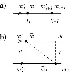
FIG. 20.: Sample diagram for illustrating the rules above. The vertical dashed lines in (b) are guides for the eye: the rules in the text are used to evaluate the piece of the diagram between times $t^{\prime}$ and $t$ that contributes to $\Sigma(t^{\prime}-t)$.

2 Energy representation

Once the rules for calculating $\Sigma$ have been laid down in time domain, it is more convenient to shift into the energy representation with respect to the phonon energies and to do this in the $d$-basis. The rule 2. remains as it is, Eq. (A5) in the rule 3. is already in the energy representation, and we only need to reformulate the first and fourth rules.

1. Propagators
   Assign a resolvent

   $$\frac{i}{\sigma\omega-E_{d^{\prime}}+E_{d}+i\eta}$$ (A13)

   to each piece of a diagram temporally between two vertices, i.e., irrespective of the propagator they lie on. Here $\omega$ is the phonon energy, and $E_{d^{\prime}}$ and $E_{d}$ are the energies of the states on the forward and backward propagators, respectively; $\sigma=+1$ $(-1)$ if the vertex with the earlier time lies on the forward (backward) propagator. The factor $\eta>0$ arises from the adiabatic turning on of the interaction and is taken to zero at the end.

1. Summations and integrations
   Sum over all internal indices and integrate over $\omega$. Due to the factor $i\eta$, the integrations are to be understood as combinations of Cauchy’s principal value integrals and delta functions.

In diagrams such as those in Fig. 21a the prefactors due to the vertices are equal. Therefore these can be pairwise combined and their integral parts written together as

$$\int_{-\infty}^{\infty}d\omega\,\Gamma(\omega)$$ (A14)

$$\;\;\;\;\;\;\cdot\left[\frac{i}{-\omega+(E_{d^{\prime}}-E_{d_{1}})+i\eta}+\frac{i}{\omega-(E_{d_{1}^{\prime}}-E_{d})+i\eta}\right].$$ (A15)

If $d^{\prime}=d_{1}^{\prime}$ and $d=d_{1}$, i.e., if the density matrix is diagonal before and after the transition, this expression simplifies into

$$\pi\int_{-\infty}^{\infty}d\omega\,\Gamma(\omega)\,\delta(\omega-(E_{d^{\prime}}-E_{d}))$$ (A16)

$$\;\;\;\;\;=\pi\,\Gamma(E_{d^{\prime}}-E_{d})=\frac{\pi A^{2}}{12\rho c^{5}\hbar^{4}}\cdot\frac{\Delta E^{3}}{e^{\beta\Delta E}-1}.$$ (A17)

In the last step we inserted the definition of $\Gamma(\omega)$ from the equation (B13) and identified $\Delta E=E_{d^{\prime}}-E_{d}$ as the energy required for the transition from the state $d$ to $d^{\prime}$. This expression, Eq. (A16), together with the prefactor $G_{d^{\prime}d,d_{1}d_{1}^{\prime}}$ is the phonon induced transition rate $\Sigma_{d,d^{\prime}}$ used in the literature and in Parts III and IV of this paper. From Eqs. (A14) and (A16) we see that the energy is only conserved (the delta function, cf. Fermi’s golden rule) under some special circumstances and, in general, the rate need not be the simple real function used in the literature.

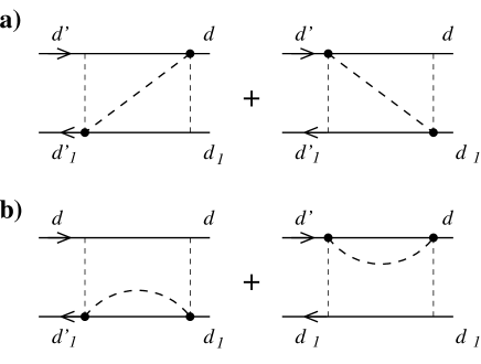
FIG. 21.: Diagrams may sometimes be pairwise combined to simplify the calculations.

B The spin-phonon rates

In this Appendix, we outline the calculation of the phonon-induced transition rates $\Sigma$ between different spin states. In order to calculate $\Sigma$ in lowest order in the spin-phonon coupling constants $g_{i}$, we need to evaluate the contractions $\langle{\mathcal{H}}_{\rm sp}(t){\mathcal{H}}_{\rm sp}(t^{\prime})\rangle_{\rm ph}$, where the expectation value is taken with respect to the phonon degrees of freedom. Let us first insert Eq. (8) into Eq. (4) and explicitly write down all the resulting terms

$${\mathcal{H}}_{\rm sp}(t)=i\sum_{\vec{k}\sigma}\sqrt{\frac{\hbar}{2MN\omega_{\vec{k}\sigma}}}[b_{\vec{k}\sigma}^{\dagger}e^{-i\omega_{\vec{k}\sigma}t}+b_{\vec{k}\sigma}e^{i\omega_{\vec{k}\sigma}t}]e^{i\vec{k}\cdot\vec{r}}$$ (B1)

$$\;\;\;\;\;\cdot\{g_{1}[S_{x}^{2}(t)-S_{y}^{2}(t)][e_{x}^{(\sigma)}k_{x}-e_{y}^{(\sigma)}k_{y}]$$ (B2)

$$\;\;\;\;\;\;\;\;+\frac{g_{2}}{4}\{S_{x}(t),S_{y}(t)\}[e_{x}^{(\sigma)}k_{y}+e_{y}^{(\sigma)}k_{x}]$$ (B3)

$$\;\;\;\;\;\;\;\;+\frac{g_{3}}{4}(\{S_{x}(t),S_{z}(t)\}[e_{x}^{(\sigma)}k_{z}+e_{z}^{(\sigma)}k_{x}]$$ (B4)

$$\;\;\;\;\;\;\;\;\;\;\;\;\;\;\;\;\;\;\;\;\;\;\;\;\;\;\;\;\;\;\;\;\;\;\;+\{S_{y}(t),S_{z}(t)\}[e_{y}^{(\sigma)}k_{z}+e_{z}^{(\sigma)}k_{y}])$$ (B5)

$$\;\;\;\;\;\;\;\;+\frac{g_{4}}{4}(\{S_{x}(t),S_{z}(t)\}[e_{x}^{(\sigma)}k_{z}-e_{z}^{(\sigma)}k_{x}]$$ (B6)

$$\;\;\;\;\;\;\;\;\;\;\;\;\;\;\;\;\;\;\;\;\;\;\;\;\;\;\;\;\;\;\;\;\;\;\;+\{S_{y}(t),S_{z}(t)\}[e_{y}^{(\sigma)}k_{z}-e_{z}^{(\sigma)}k_{y}])\}.$$ (B7)

In evaluating the contraction, we need to consider all the possible states before and after the action of ${\mathcal{H}}_{\rm sp}(t^{(\prime)})$ as well as all the possible orderings of the times $t$ and $t^{\prime}$ along the contour. As a characteristic example, let us consider the diagram in Fig. 20b and hold to the same usage of indices. The time dependences of the spin operators are accounted for by the propagators and they can be put aside for the moment. The remaining part with the spin operators is fully determined by the spin states before and after the vertices yielding

$$\langle\bar{m}_{1}|S^{\xi^{\prime}}|m_{1}\rangle\cdot\langle\bar{m}|S^{\xi}|m^{\prime}\rangle=\sqrt{S_{\bar{m},m^{\prime}}S_{m_{1},\bar{m}_{1}}}.$$ (B8)

Here $\xi=\bar{m}-m^{\prime},\xi^{\prime}=m_{1}-\bar{m}_{1}$ can take values $\pm 1$ or $\pm 2$ due to the structure of ${\mathcal{H}}_{\rm sp}$, and, for brevity, $S^{\pm|\xi|}\equiv S_{\pm}^{|\xi|}$. The quantities on the right hand side of the equation are

$$S_{\bar{m},m^{\prime}}=(2m^{\prime}+\xi)\sqrt{S(S+1)-m^{\prime}(m^{\prime}+\xi)}$$ (B9)

for $\xi=\pm 1$ or

$$S_{\bar{m},m^{\prime}} = \left\{\left[S(S+1)-m^{\prime}(m^{\prime}+\nu)\right]\right.$$ (B11)

$$\;\;\;\;\;\;\;\;\;\;\left.\left[S(S+1)-(m^{\prime}+\nu)(m^{\prime}+2\nu)\right]\right\}^{1/2}$$

for $\xi=\pm 2$, $\nu=sign(\xi)$.

The part of the contraction depending on the phonon degrees of freedom is evaluated assuming acoustic phonons with a linear dispersion relation and three modes indexed by $\sigma=1,2,3$ (one longitudinal and two transverse modes). The polarization vectors $e_{\alpha}^{(\sigma)}$ are assumed unit vectors. The resulting expression consists of two parts. The first one of them contains all the information concerning the phonon spectrum, energies, and temperature,

$$\Gamma(t-t^{\prime}) = \int_{-\infty}^{\infty}d\omega\;\Gamma(\omega)\;e^{i\omega(t-t^{\prime})}$$ (B12)

$$\equiv \int_{-\infty}^{\infty}d\omega\frac{A^{2}}{12\rho c^{5}\hbar^{4}}\cdot\frac{\omega^{3}}{e^{\beta\omega}-1}\cdot e^{i\omega(t-t^{\prime})}.$$ (B13)

This part is defined such that it is independent of the spin states and only contains the term $A^{2}$ from the coupling constants that turns out to be constant for all the rates. In the diagrams, this corresponds to the spin-phonon interaction line. The second part,

$$C_{\xi,\xi^{\prime}}=\left\{\begin{array}[]{clrr}0,&{\rm for}|\xi|\neq|\xi^{\prime}|\\[4.0pt] 1,&\xi=\xi^{\prime}=\pm 1\\[4.0pt] \frac{15}{16}+\frac{1}{8}\delta_{\xi,\xi^{\prime}},&|\xi|=|\xi^{\prime}|=2\end{array}\right.,$$ (B17)

however, does depend on the spin states and implies additional selection rules. It should be noted that the third clause allows for $\xi\neq\xi^{\prime}$ if $|\xi|=|\xi^{\prime}|=2$. For convenience, we combine the term $C_{\xi,\xi^{\prime}}$ with the spin operators and obtain the term

$$G_{\bar{m}m^{\prime},m_{1}\bar{m}_{1}}=\sqrt{S_{\bar{m},m^{\prime}}S_{m_{1},\bar{m}_{1}}}\cdot C_{\xi,\xi^{\prime}},$$ (B18)

which in the diagrammatic language corresponds to a pair of vertices.

In the $d$-basis, the time dependence of the spin operators is of a simple exponential form, cf. Eq. (A3), and the diagram in Fig. 20b can be evaluated to yield

$$\Sigma(t-t^{\prime})_{mm_{1},m^{\prime}m_{1}^{\prime}}=$$ (B19)

$$\;\;\;\;\sum_{\bar{m},\bar{m}_{1}}G_{\bar{m}m^{\prime},m_{1}\bar{m}_{1}}\cdot\sum_{d,d_{1}}\langle m_{1}^{\prime}|d_{1}\rangle\langle d_{1}|m_{1}\rangle\langle m|d\rangle\langle d|\bar{m}\rangle$$ (B20)

$$\;\;\;\;\;\;\;\;\;\;\;\;\;\;\;\;\;\;\;\;\;\;\;\;\;\;\;\;\;\;\;\;\;\;\;\;\;\;\;\;\;\;\cdot e^{-i(E_{d}-E_{d^{\prime}})(t-t^{\prime})}\;\Gamma(t^{\prime}-t).$$ (B21)

The actual transition rates are obtained by integrating Eq. (B19) over the time difference $\tau=t-t^{\prime}$. This takes us to the energy representation, combining the exponential factor in Eq. (B19) with the $e^{i\omega(t-t^{\prime})}$ of the Fourier transform in Eq. (B13). The intergration over $\tau$ yields

$$\Sigma_{mm_{1},m^{\prime}m_{1}^{\prime}}=$$ (B22)

$$\;\;\;\;\sum_{\bar{m},\bar{m}_{1}}G_{\bar{m}m^{\prime},m_{1}\bar{m}_{1}}\cdot\sum_{d,d_{1}}\langle m_{1}^{\prime}|d_{1}\rangle\langle d_{1}|m_{1}\rangle\langle m|d\rangle\langle d|\bar{m}\rangle$$ (B23)

$$\;\;\;\;\;\;\;\;\;\;\;\;\;\;\;\;\;\;\;\;\;\;\;\;\;\;\;\;\;\;\;\;\;\;\;\;\;\cdot i\int_{-\infty}^{\infty}d\omega\frac{\Gamma(\omega)}{-\omega-E_{d}+E_{d^{\prime}}+i\eta}.$$ (B24)

As the final step in calculating $\Sigma$, let us evaluate the integral in Eq. (B22) or

$$\tilde{I}_{\sigma}(\Delta E,\beta) =\int_{-\infty}^{\infty}d\omega\frac{\omega^{3}}{e^{\beta\omega}-1}\cdot\frac{1}{\sigma(\omega-\Delta E)+i\eta}$$ (B25)

$$= P\int_{-\infty}^{\infty}d\omega\frac{\omega^{3}}{e^{\beta\omega}-1}\cdot\frac{1}{\sigma(\omega-\Delta E)}-i\pi\frac{\Delta E^{3}}{e^{\beta\Delta E}-1}$$ (B26)

for the general case. Here $\sigma=\pm 1$. The imaginary part of the integral (the last term) is, up to a prefactor, just $-i\pi\Gamma(\Delta E)$ and is independent of $\sigma$. The real part in turn can be evaluated using the calculus of residues. By combining the integral along the real axis with an infinite semicircle in the upper half plane to form a closed contour we obtain ${\rm Re}\{\tilde{I}_{\sigma}(\Delta E,\beta)\}=-2\pi{\rm Im}\sum\{enclosed\;{\rm residues}\}$.

The real part of the integral $\tilde{I}_{\sigma}(\Delta E,\beta)$ is divergent due to the $\omega^{3}$-term and some kind of a cutoff procedure is needed here. We have chosen a functional cutoff using instead of $\tilde{I}(\Delta E,\beta)$ the integral

$$I_{\sigma}(\Delta E,\beta,D)=$$ (B27)

$$\;\;\;\;\;\;\int_{-\infty}^{\infty}d\omega\frac{\omega^{3}}{e^{\beta\omega}-1}\cdot\frac{1}{\sigma(\omega-\Delta E)+i\eta}\cdot\left(\frac{D^{2}}{D^{2}+\omega^{2}}\right)^{2},$$ (B28)

i.e., the cutoff function is a Lorentzian squared and the additional parameter $D$ is the cutoff parameter of the Lorentzian. The integrand in (B27) has single poles at $\omega=\Delta E-i\sigma\eta$, and at $\omega=2m\pi i/\beta$, where $m$ is a positive integer; there are also second-order poles at $\omega=\pm iD$. The residues $C^{(1)}$ from the first pole are real and can be neglected. Collecting the other poles in the upper half plane and evaluating the residues yields

$${\rm Re}\left\{I_{\sigma}(\Delta E,\beta,D)\right\}=-2\pi\left[\sum_{m=1}^{\infty}C_{m}^{(2)}+C^{(3)}\right],$$ (B29)

where

(B30)

$$C_{m}^{(2)}=\sigma\frac{\beta^{2}\Delta ED^{4}}{(2\pi)^{3}}\cdot\frac{m^{3}}{\left(\frac{\Delta E\beta}{2\pi}\right)^{2}+m^{2}}\cdot\frac{1}{\left[\left(\frac{D\beta}{2\pi}\right)^{2}-m^{2}\right]^{2}}$$ (B31)

$$C^{(3)}=-\sigma\frac{D^{5}}{4(\Delta E^{2}+D^{2})}\Bigg{[}\frac{\beta\Delta E}{4\sin^{2}\left(\frac{\beta D}{2}\right)}$$ (B32)

$$\;\;\;\;\;\;\;\;-\frac{1}{\Delta E^{2}+D^{2}}\left(\frac{3}{2}\Delta E^{2}+\frac{1}{2}D^{2}+\frac{\Delta E^{3}}{D}\cot\left(\frac{\beta D}{2}\right)\right)\Bigg{]}.$$ (B33)

If $D$ is accidentally chosen to equal $2\pi m^{*}/\beta$ for some $m^{*}$, the residues $C_{m^{*}}^{(2)}+C^{(3)}$ should be replaced by

$$C^{*}=\sigma\frac{D^{3}}{16\beta}\cdot\frac{3\Delta E^{5}-14\Delta E^{3}D^{2}-\Delta ED^{4}}{(\Delta E^{2}+D^{2})^{3}}.$$ (B34)

In the $d$-basis and using only the diagonal elements of the reduced density matrix, the integrals $I_{\sigma}(\Delta E,\beta,D)$ can always be combined such that their real parts cancel each other. When using the nondiagonal elements of $\rho(t)_{d,d^{\prime}}$, as well, this is no longer true and the real parts of $I_{\sigma}(\Delta E,\beta,D)$ give rise to $D$-dependent shifts in the energies $E_{d}$. In this work, we have used $D$’s of the order of the anisotropy barrier, i.e., 50-100K, and found that this yields tiny shifts also in the relaxation rate curves but leaves the qualitative picture unchanged. In the figures in the section IV, $D$ is chosen as low as 25K in order to simplify the comparison between the calculations with and without the nondiagonal elements.

With all the contributions to $\Sigma$ written down, we can find an estimate for the order of magnitude of the elements (the individual rates) $\Sigma_{mm_{1},m^{\prime}m_{1}^{\prime}}$. The most interesting piece of information for each state is the largest rate coupling that state to other states – this rate plays a key role in justifying the neglect of the nondiagonal states in $\rho(t)$, see App. C, as well as in the suppression of the narrow resonances found in the text.

The prefactor in $\Gamma(\omega)$, cf. Eq. (B13), amounts to $7.0\cdot 10^{5}c^{-5}{\rm s}^{5}{\rm m}^{-5}{\rm K}^{-2}$, where the sound velocity $c$ is expressed in meters per second. The units are chosen such that, when $\omega$ is expressed in kelvin, also $\Gamma(\omega)$ is given in kelvin. For $\omega>0$ (and also $\omega>k_{\rm B}T$), i.e., for transitions related with phonon absorption, the energy-dependent part of $\Gamma(\omega)$ strongly decreases for increasing $\omega$; for $\omega<0$, corresponding to phonon emission, $\Gamma(\omega)$ approaches the temperature-independent power-law dependence $\omega^{3}$. The largest $\Gamma(\omega)$’s are attained for these latter processes in connection with low-energy spin states. The contribution from the spin operators, cf. Eq.(B8), on the other hand, is larger for spin states closest to the top of the barrier and tends to balance the changes in $\Gamma(\omega)$ and reduce the variations in $\Sigma_{mm_{1},m^{\prime}m_{1}^{\prime}}$ for different states and for varying $H_{z}$. The typical energy scale arising from the spin-phonon rates is found to be $10^{-5}-10^{-4}$K.

C Choice of basis

In sections III A and III B, we decidedly formulated the more general equations independent of the chosen basis for ${\mathcal{H}}_{S}$. In this appendix, we consider the eigenbases of ${\mathcal{H}}_{S}$ or the $d$-basis, in more detail.

The (strong) tunneling poses a problem for the diagrammatic formulation in the $m$-basis, but this can be easily solved by first diagonalizing ${\mathcal{H}}_{S}$ and then expressing all the equations in its eigenbasis. In this $d$-basis, the kinetic equation for the diagonal and off-diagonal density matrix elements reads

$$\dot{\rho}(t)_{d,d} = \sum_{d_{1},d_{1}^{\prime}}\!\Sigma_{dd,d_{1}d_{1}^{\prime}}\rho(t)_{d_{1},d_{1}^{\prime}}$$ (C1)

and

$$\dot{\rho}(t)_{d,d^{\prime}} = -i(E_{d}\!-\!E_{d^{\prime}})\rho(t)_{d,d^{\prime}}\!+\!\!\sum_{d_{1},d_{1}^{\prime}}\!\Sigma_{dd^{\prime},d_{1}d_{1}^{\prime}}\rho(t)_{d_{1},d_{1}^{\prime}},$$ (C2)

respectively. From the knowledge of (the full) $\rho(t)$ we can again obtain, e.g., the magnetization

$$M(t) = g\,\mu_{\rm B}\sum_{d,d^{\prime}}\sum_{m}\,\langle d^{\prime}|m\rangle\,m\,\langle m|\,d\rangle\,\rho_{d,d^{\prime}}(t)$$ (C3)

$$\equiv g\,\mu_{\rm B}\sum_{d,d^{\prime}}m_{d,d^{\prime}}\rho_{d,d^{\prime}}(t)$$ (C4)

where $m_{d,d^{\prime}}$ is defined in this way as the matrix element of $S_{z}$ in the $d$-basis.

When the tunneling rates dominate the kinetic equations, the main features of the eigenstates can be understood in even simpler terms as follows. When a given state is off-resonant, there is essentially a one-to-one correspondence between each of the $m$- and $d$-states, i.e., also the $d$-states are localized on one or the other side of the barrier. Close to a resonance, two states $m_{l}$ and $m_{r}$ on different sides of the barrier, see Fig. 22, get coupled and form an approximate two-state system described by

$${\mathcal{H}}_{2}=\left(\begin{array}[]{clrr}E_{m_{l}}&\Delta\\ \Delta^{*}&E_{m_{r}}\end{array}\right).$$ (C7)

The nondiagonal elements denote the tunnel splitting as obtained from the diagonalization of the full spin Hamiltonian; the subscripts stand for the left and right sides of the barrier. The eigensolutions to this are the symmetric and antisymmetric combinations of the respective $m$-states

$$|d_{s}\rangle = \alpha|m_{l}\rangle+\beta|m_{r}\rangle$$ (C8)

$$|d_{a}\rangle = \beta|m_{l}\rangle-\alpha|m_{r}\rangle$$ (C9)

that extend through the barrier, see Fig. 22. The factors $\alpha$ and $\beta$ are the normalized constants

$$\alpha = \frac{\Delta}{\sqrt{\hat{\varepsilon}^{2}+|\Delta|^{2}}}$$ (C10)

$$\beta = \frac{\hat{\varepsilon}}{\sqrt{\hat{\varepsilon}^{2}+|\Delta|^{2}}}$$ (C11)

with $\hat{\varepsilon}=\frac{1}{2}[(E_{l}-E_{r})-\sqrt{(E_{l}-E_{r})^{2}+4|\Delta|^{2}}]$.

The biggest simplification is attained when we argue that, for the most values of $H_{z}$, we can restrict our considerations to the diagonal elements of the density matrix. A naive justification for this concerns the stationary values of the density matrix elements [obtained by requiring $\dot{\rho}(t)_{d,d^{\prime}}=0$]. This leads to the immediate conclusion that all the off-diagonal elements between nonresonant states are negligibly small. Furthermore, the nondiagonal elements are also very small for any pair of resonant states as long as the tunnel splitting of that particular resonance is larger than the spin-phonon rates coupling these states to others, see the end of App. B.

We also investigated the temporal behaviour of the off-diagonal elements in terms of the reduced model shown in Fig. 22 and the results lend support to the above conclusions. The idea of this simulation was to prepare the system into the state $d_{i}$ at the initial time $t_{0}$, let the system then evolve in time according to the kinetic equation, and see how the off-diagonal elements $\rho(t)_{d_{s},d_{a}}$ and $\rho(t)_{d_{a},d_{s}}$ behave. The resonant pair of states in the figure is similar to the one in Eqs. (C8) and (C9) and it is coupled to two lower, nonresonant states $d_{i}$ and $d_{f}$. The rates depicted in the figure are $\Sigma_{u}=\Sigma_{ll,ii}$ and $\Sigma_{d}\approx(\Sigma_{ii,ll}+\Sigma_{ff,rr})/2$. The magnitudes of these rates – as compared to the tunnel splitting $|2\Delta|$ – determine two regimes. If $2|\Delta|\gg\Sigma_{\rm d}$, the amplitudes of the nondiagonal elements are found to quickly reach their maxima $\propto\Sigma_{\rm u}/|2\Delta|$ and their values orbit around and “decay” towards the respective complex stationary values. On the other hand, according to the detailed-balance relation, the stationary values of the diagonal elements are proportional to $\Sigma_{\rm u}/\Sigma_{\rm d}$. Hence $\rho(t)_{d,d^{\prime}}/\rho(t)_{d^{(\prime)}}\propto\Sigma_{\rm d}/|2\Delta|$ and we can neglect the nondiagonal elements, if $\Sigma_{\rm d}\ll 2|\Delta|$. In this case the kinetic equation, Eqs. (C1) and (C2), becomes very simple: Eq. (C2) can be neglected and the rate $\Sigma$ acquires the form, cf. App. B,

$$\Sigma_{d^{\prime}d^{\prime},dd}=\pm G_{dd^{\prime},d^{\prime}d}\,\frac{\pi A^{2}}{12\rho c^{5}\hbar^{4}}\cdot\frac{\Delta E^{3}}{e^{\beta\Delta E}-1},$$ (C12)

where

$$G_{dd^{\prime},d^{\prime}d} = \!\sum_{m_{1},m_{2}}\sum_{m_{3},m_{4}}\!\!\!G_{m_{4}m_{3},m_{2}m_{1}}$$ (C14)

$$\;\;\;\;\;\;\;\;\;\;\;\;\;\;\;\;\;\;\;\;\;\;\;\;\;\cdot\langle d^{\prime}|m_{4}\rangle\langle m_{3}|d\rangle\langle d|m_{2}\rangle\langle m_{1}|d^{\prime}\rangle$$

corresponds to the vertices and contains the spin-phonon coupling constants, see App. A. In the opposite case, $2|\Delta|\ll\Sigma_{\rm d}$, the nondiagonal elements do not perform orbiting motion in the complex plane but increase motonously to roughly one half of $\rho_{d^{(\prime)}}^{(0)}$. In this case, the off-diagonal elements clearly cannot be neglected.

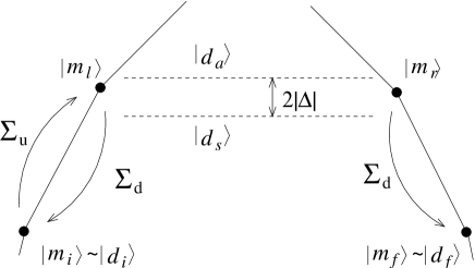
FIG. 22.: Schematic of the situation discussed in the text. If the spin-phonon coupling denoted by the arrows and $\Sigma$’s is much weaker than the tunnel coupling $\Delta$ between the states $|m_{l}\rangle$ and $|m_{r}\rangle$, these states can be thought of as an effective two-state system. The eigenstates of the two-state system are depicted as dashed lines separated in energy by $2|\Delta|$. The subscripts of the $\Sigma$’s correspond to those used in the text.

For Mn₁₂ we can attain the whole range of cases: for the most strongly coupled level(s) $2|\Delta|\gg\Sigma_{\rm d}$, while for the lower levels, $2|\Delta|\ll\Sigma_{\rm d}$. In the former case, the diagonal elements $\rho_{d}(t)$ are sufficient in describing the system whereas, in the latter case, we either have to include the nondiagonal states or restrict our considerations to magnetic fields for which $\Delta E\gg\Sigma_{\rm d}$ for all the levels, cf. Ref. [16]. In the text, we neglect the nondiagonal elements in the calculation of $\chi(\omega)$ and in some of the analytical considerations but compare the two cases in section IV.

D Laplace transformation

In this appendix, we consider the Laplace tranformation

$$f(z)\equiv\int_{0}^{\infty}\!\!dt\,e^{-izt}f(t)$$ (D1)

of the kinetic equation, Eq. (20). We also give another proof of the applicability of the Markov approximation in calculating the relaxation rates.

The kinetic equation is readily transformed into

$$-iz\rho(z)-\rho(t = 0)=-iL_{0}\,\rho(z)+\Sigma(z)\rho(z)$$ (D2)

$$\Rightarrow\rho(z) = \frac{\rho(t=0)}{-iz+iL_{0}-\Sigma(z)}.$$ (D3)

The poles of Eq. (D3), i.e., the solutions of $-iz_{i}+iL_{0}-\Sigma(z_{i})=0$, yield the exact eigenvalues to the kinetic equation: $z_{i}=\omega_{i}+i/\tau_{i}$. For the slowest mode of the time evolution, one can consider the expansion

$$\Sigma(z_{1})\approx\Sigma(0)+z_{1}\cdot\frac{\partial\Sigma(z)}{\partial z}\Big{|}_{z=0}+...$$ (D4)

The prefactor of the $z_{1}$ may be evaluated to be proportional to $[\tau_{1}\cdot\min\{\Delta E,k_{\rm B}T,D\}]^{-1}$, i.e., to the maximal ratio between the over-barrier relaxation rate $1/\tau_{1}$ and the other characteristic energy scales in the problem: level spacing and/or splitting $\Delta E$, temperature $k_{\rm B}T$, and the cutoff of the phonon spectrum $D$ (the cutoff $D$ is introduced in order to assure that the real part of Eq. (A14) is convergent also when we consider the nondiagonal density matrix elements). It turns out that the actual relaxation rates are several orders of magnitude smaller than any other energy scale and it becomes safe to approximate

$$\rho(z)\approx\frac{\rho(t=0)}{-iz+iL_{0}-\Sigma(0)}=\frac{\rho(t=0)}{-iz-W}$$ (D5)

where $\Sigma(0)$ has been identified as the constant $\Sigma$ of the Markov approximation above and $W$ is defined accordingly, cf. Eq. (21). This approximation is valid for the relaxation mode and time $\tau_{1}$

$$\rho^{(1)}(z)=\frac{\rho^{(1)}(t=0)}{-iz-1/\tau_{1}}$$ (D6)

but the Markov approximation may give erroneous results for the faster eigenmodes for which Eq. (D5) no longer holds true.

E Lorentzian peak shapes

The series of peaks found in the relaxation rates/times, cf. Fig. 9, may be understood in terms of different relaxation paths, each path with a possible tunneling channel giving rise to a peak – see [18] for nice illustrations of the paths. In this appendix, we sketch a derivation that aims to show that the Lorentzian peak shapes are actually something to be expected.

When the spin system is somehow disturbed away from equilibrium and then let relax, it quickly acquires a metastable state, a thermal equilibrium separately on each side of the barrier. This initial thermalization into the metastable state is driven by the spin-phonon interaction that can change the spin states $m$ by $\pm 1$ or $\pm 2$. At a much longer time scale, the system relaxes over the barrier towards the real equilibrium configuration. For the relaxation to take place, the crucial step is the final transition that transfers the spin onto the other side of the barrier. We can distinguish two regimes in terms of how this critical transition takes place. In absence of tunneling, e.g., in off-resonance conditions, the relaxation is only possible over the top of the barrier, while for relatively strong tunnel splitting and for resonant conditions, the dominant path is via tunneling across the barrier well below its top. When the tunneling is weak compared with the spin-phonon interaction, the tunneling rate is the bottle neck for the relaxation to take place. In Mn₁₂, this is the case for tunneling between the low-lying states with $|m|>4$ (for $H_{z}\approx 0$T). However, for the experimentally relevant resonances, the tunneling is strong and takes place between the higher states. In this case, the spin actually oscillates back and forth through the barrier until it relaxes to some lower state on either side of the barrier. This is the case of interest here.

In the strong-tunneling regime, the system is best described in terms of the $d$-basis where it suffices to consider the diagonal elements of the density matrix. In order to get a more intuitive picture of the relaxation, let us consider a situation where the system has been prepared onto one side of the barrier and has reached the metastable thermal equilibrium there. This initial condition is convenient for two purposes: first, the relaxation only proceeds into one direction and, second, the phonon-induced transitions on this one side of the barrier are accounted for by the thermal probabilities $\tilde{\rho}_{d}$ (tilde denotes the metastable state and we write just one index for the diagonal matrix elements). Let us further consider relaxation via a single tunneling resonance and take into account the states and transition processes illustrated in Fig. 23. The system starts in the initial state $d_{i}$ (localized onto the left side of the barrier, $\sim m_{i}$), is then activated onto resonance into either the symmetric or antisymmetric state, denoted by $d_{s}$ and $d_{a}$, respectively, and at some point is transfered down to the final state $d_{f}$ (localized onto the right side of the barrier, $\sim m_{f}$). The subsequent intravalley relaxation is so fast that after the transition to $d_{f}$ the relaxation can be considered complete. The states $d_{s}$ and $d_{a}$ extend through the barrier and this is the key point of the present discussion: the spin is transferred through the barrier in a single step, the rate being determined by thermal activation but also by the magnetic-field dependent amplitudes $\alpha$ and $\beta$, from Eqs. (C8) and (C9), for the two extended states to be on either side of the barrier. These amplitudes determine the relative probabilities for the activation process to couple to the resonant states.

FIG. 23.: Illustration of the parameters discussed in the text: states in the $m$ and $d$-bases, transition rates $\Sigma_{m,m^{\prime}}$, and factors $\pm\alpha$ and $\beta$ from Eq. (C7).

The above discussion can be formulated in the language of a master equation:

$$\dot{\tilde{\rho}}_{d_{s}}(t)=0 \approx \Sigma_{d_{s},d_{i}}\tilde{\rho}_{d_{i}}(t)-(\Sigma_{d_{f},d_{s}}+\Sigma_{d_{i},d_{s}})\tilde{\rho}_{d_{s}}(t)$$ (E5)

$$\!\!\!\!\!\!\!\!\!\!\approx|\langle d_{s}|m_{l}\rangle|^{2}\Sigma_{m_{l},m_{i}}\tilde{\rho}_{d_{i}}(t)$$

$$\!\!\!\!\!\!\!\!\!\!-(|\langle d_{s}|m_{r}\rangle|^{2}\Sigma_{m_{f},m_{r}}\!+|\langle d_{s}|m_{l}\rangle|^{2}\Sigma_{m_{i},m_{l}})\tilde{\rho}_{d_{s}}(t)$$

$$\!\!\!\!\!\!\!\!\!\!=|\alpha|^{2}\Sigma_{m_{l},m_{i}}\tilde{\rho}_{d_{i}}(t)$$

$$\;\;\;\;\;\;\;\;\;\;-(|\beta|^{2}\Sigma_{m_{f},m_{r}}+|\alpha|^{2}\Sigma_{m_{i},m_{l}})\tilde{\rho}_{d_{s}}(t)$$

$$\dot{\tilde{\rho}}_{d_{a}}(t)=0 \approx \Sigma_{d_{a},d_{i}}\tilde{\rho}_{d_{i}}(t)-(\Sigma_{d_{f},d_{a}}+\Sigma_{d_{i},d_{a}})\tilde{\rho}_{d_{a}}(t)$$ (E10)

$$\!\!\!\!\!\!\!\!\!\!\approx|\langle d_{a}|m_{l}\rangle|^{2}\Sigma_{m_{l},m_{i}}\tilde{\rho}_{d_{i}}(t)$$

$$\!\!\!\!\!\!\!\!\!\!-(|\langle d_{a}|m_{r}\rangle|^{2}\Sigma_{m_{f},m_{r}}\!+|\langle d_{a}|m_{l}\rangle|^{2}\Sigma_{m_{i},m_{l}})\tilde{\rho}_{d_{a}}(t)$$

$$\!\!\!\!\!\!\!\!\!\!=|\beta|^{2}\Sigma_{m_{l},m_{i}}\tilde{\rho}_{d_{i}}(t)$$

$$\;\;\;\;\;\;\;\;\;\;-(|\alpha|^{2}\Sigma_{m_{f},m_{r}}+|\beta|^{2}\Sigma_{m_{i},m_{l}})\tilde{\rho}_{d_{a}}(t).$$

The approximate equalities are just a reminder that we have neglected, e.g., the contributions from states above the resonance as well as the return possibility from state $d_{f}$. These equations can be simplified by the assumption $\Sigma_{m_{i},m_{l}}\approx\Sigma_{m_{f},m_{r}}$ which is reasonable for a pair of resonant states – as a result, the $\Sigma$’s can be taken out of the brackets in the last forms of the above formulas. By further noting that due to normalization $|\alpha|^{2}+|\beta|^{2}=1$ and that the resulting probabilities are time independent, we obtain

$$\tilde{\rho}_{d_{s}} \approx |\alpha|^{2}\,\frac{\Sigma_{m_{l},m_{i}}}{\Sigma_{m_{i},m_{l}}}\,\tilde{\rho}_{d_{i}}$$ (E11)

$$\tilde{\rho}_{d_{a}} \approx |\beta|^{2}\,\frac{\Sigma_{m_{l},m_{i}}}{\Sigma_{m_{i},m_{l}}}\,\tilde{\rho}_{d_{i}}.$$ (E12)

The ratio of the $\Sigma$’s is just the thermal factor $\exp[-\beta(E_{l}-E_{i})]$, cf. detailed balance, and $\tilde{\rho}_{d_{i}}$ is the thermal probability to be in a state with energy $E_{i}$ over the lowest energy $E_{-10}$ on left hand side (for $H_{z}>0$). Together these yield a factor $c\cdot\exp[-\beta(E_{l}-E_{-10})]$, where $c$ is a normalization constant equal to $\tilde{\rho}_{-10}$ which is close to unity for the temperatures of interest.

In the next and final step, the relaxation rate is obtained from the knowledge of these probabilities and the rates to be dragged down on the right hand side of the barrier, i.e.,

$$\tau^{-1} \approx \Sigma_{d_{f},d_{s}}\cdot\tilde{\rho}_{d_{s}}+\Sigma_{d_{f},d_{a}}\cdot\tilde{\rho}_{d_{a}}$$ (E13)

$$\approx |\beta|^{2}\Sigma_{m_{f},m_{r}}\,\tilde{\rho}_{d_{s}}+|\alpha|^{2}\Sigma_{m_{f},m_{r}}\,\tilde{\rho}_{d_{a}}$$ (E14)

$$\approx 2\,|\alpha|^{2}|\beta|^{2}\,\Sigma_{m_{f},m_{r}}\,c\cdot e^{-\beta(E_{i}-E_{-10})}.$$ (E15)

The exponential factor is just the effective Arrhenius factor seen in experiments, $\frac{1}{2}\,c\,\Sigma_{m_{f},m_{r}}=\tau_{0}^{-1}$, and

$$4\,|\alpha|^{2}|\beta|^{2}=\frac{(2|\Delta|)^{2}}{(E_{m_{l}}-E_{m_{r}})^{2}+(2|\Delta|)^{2}}.$$ (E16)

Here $2|\Delta|$ is the tunnel splitting. It is more or less independent of $H_{z}$ but $\xi\equiv E_{m_{l}}-E_{m_{r}}$ can be tuned with the magnetic field. In terms of the field, the width of the resonant peak at its half maximum is

$$\delta H_{z}=\frac{4|\Delta|}{g\mu_{\rm B}|m_{l}-m_{r}|}.$$ (E17)

This sketch of a derivation introduces all the factors seen in experiments: the Arrhenius law with a reasonable prefactor $\tau_{0}^{-1}$, that depends weakly on temperature and the particular resonance, see the two last paragraphs of App. B, and peaks of accelerated relaxation superimposed on it. The peak heights or the relaxation rates on resonance are found to correspond to the Boltzmann or Arrhenius factor with the energy corresponding to the effective barrier height. The peak shape is Lorentzian as observed in experiment with widths given by precisely the tunnel splittings.

REFERENCES

- [1] J.R. Friedman et al., Phys. Rev. Lett. 76, 3830 (1996).
- [2] J.M. Hernandez et al., Europhys. Lett. 35, 301 (1996).
- [3] L. Thomas et al., Nature (London) 383, 145 (1996).
- [4] J.M. Hernandez et al., Phys. Rev. B 55, 5858 (1997).
- [5] F. Luis et al., Phys. Rev. B 55, 11 448 (1997).
- [6] A. Ganeschi, D. Gatteschi, and R. Sessoli, J. Am. Chem. Soc. 113, 5873 (1991); R. Sessoli et al., Nature (London) 365, 141 (1993).
- [7] R. Sessoli, Mol. Cryst. Liq. Cryst. 274, 145 (1995).
- [8] Some authors do report possible observations of dipolar effects, especially at low temperature, see e.g. Refs. [15] and [33].
- [9] The division between thermally-activated and tunneling-enhanced relaxation depends on typical experimental time scales. In relaxation measurements, the magnetization first relaxes faster than exponentially and only asymptotically reaches an exponential regime. For , almost all the spins relax before reaching this stage. In susceptibility experiments, on the other hand, the relevant time scale is the measurement frequency and this can keep up with the relaxation rate up to 5-6K.
- [10] J. Villain et al., Europhys. Lett. 27, 159, (1994).
- [11] P. Politi et al, Phys. Rev. Lett. 75, 537 (1995).
- [12] F. Hartman-Boutron, P. Politi, and J. Villain, Int. J. Mod. Phys. B 10, 2577 (1996).
- [13] M.A. Novak and R. Sessoli, in Quantum Tunneling of Magnetization, edited by L. Gunther and B. Barbara (Kluwer, Dordrecht, 1995).
- [14] D.A. Garanin and E.M. Chudnovsky, Phys. Rev. B 56, 11 102 (1997).
- [15] L. Thomas, A. Caneschi, and B. Barbara, Phys. Rev. Lett. 83, 2398 (1999).
- [16] F. Luis, J. Bartolome, and J.F. Fernandez, Phys. Rev. B 57, 505 (1998).
- [17] A. Fort et al, Phys. Rev. Lett. 80, 612 (1998).
- [18] M.N. Leuenberger and D. Loss, Europhys. Lett. 46, 692 (1999); preprint cond-mat/9907154.
- [19] N.V. Prokof’ev and P.C.E. Stamp, Phys. Rev. Lett. 80, 5794 (1998).
- [20] T. Ohm, C. Sangregorio, and C. Paulsen, Eur. Phys. J. B 6, 195 (1998); J. Low Temp. Phys. 113, 1141 (1998).
- [21] D.A. Garanin, E.M. Chudnovsky, and R. Schilling, preprint cond-mat/9911055.
- [22] M. Al-Saqer et al., preprint cond-mat/9909278.
- [23] I. Tupitsyn and B. Barbara, preprint cond-mat/0002180.
- [24] T. Pohjola and H. Schoeller, in proceedings of LT22, to appear in Physica B.
- [25] A.D. Kent it et al., preprint cond-mat/9908348 – submitted to Europhys. Lett.; Y. Zhong and M. Sarachik report observing side resonances also in relaxation measurements, private communication – to be published.
- [26] A.L. Barra, D. Gatteschi, and R. Sessoli, Phys. Rev. B 56, 8192 (1997).
- [27] Y. Zhong et al., J. Appl. Phys. 85, 5636 (1999).
- [28] R. Sessoli et al., J. Am. Chem. Soc. 115, 1804 (1993).
- [29] This bears analogy to the related molecular magnet Fe8, which has hard, medium, and easy axes – the interference effects in the tunnel splittings appear when the external magnetic field is oriented parallel to the hard axis.
- [30] Similar results were recently reported in Ref. [23]; see Ref. [31] for a detailed analysis of the interference effects.
- [31] M.N. Leuenberger and D. Loss, to be published.
- [32] In Ref. [22] the authors calculate the energy spectrum for Mn12 starting from the twelve atomary spins and find different level splittings to those predicted by the simple model. The discrepancy varies between different pairs of states and as ratio varies between 0.8 to 5 from higer to lower states, respectively. Such details do not affect the essence of this paper and may be inserted as parameters into the calculation.
- [33] W. Wernsdorfer, R. Sessoli, and D. Gatteschi, Europhys. Lett. 47, 254 (1999).
- [34] D.A. Garanin, J. Phys. A 24, L61 (1991).
- [35] H. Schoeller and G. Schön, Phys. Rev. B 50, 18436 (1994); J. König et al., Phys. Rev. B 54, 16820 (1996).
- [36] Rigorously taken, instead of , we should use and insert this into Eq. (20). Combining the exponential factors yields the expressions of Refs. [41] and [18]. This procedure complicates the correspondence of the indices in the equations and in the diagrams, and, as this is found to make very little difference to the final results, [37] we neglect this step here.
- [37] We performed the calculation with both kinds of Markov approximations and the results did not show any significant differences. It is also noteworthy that when using only the diagonal states of the eigenbasis the two approximations become equal.
- [38] We have solved the problem numerically for the full density matrix in both bases, i.e., either first diagonalizing the spin part or taking the tunneling matrix elements into account to all orders in the -basis. The results are of course equivalent.
- [39] R. Kubo, M. Toda, and N. Hashitsume, Statistical Physics II, Nonequilibrium Statistical Mechanics, Springer, 1985.
- [40] E. Chudnovsky and J. Tejada, Macroscopic Quantum Tunneling of the Magnetic Moment, Cambridge, 1998, ch. 6.
- [41] K. Blum, Density Matrix Theory and Applications, 2nd edition, Plenum Press, 1996, ch. 8.
- [42] G. Belessa et al., Phys. Rev. Lett. 83, 416 (1999).
- [43] The discussion on the decoherence is relevant for the low-lying states with small tunnel splittings.
- [44] W. Wernsdorfer and R. Sessoli, Science 284, 133 (1999).
- [45] D. Loss, D.P. DiVincenzo, and G. Grinstein, Phys. Rev. Lett. 69, 3232 (1992); J. von Delft and C.L. Henley, Phys. Rev. Lett. 69, 3236 (1992).
- [46] A. Garg, Europhys. Lett. 22, 205 (1993).
- [47] W. Wernsdorfer, contribution to the proceedings of LT22, Helsinki, to appear in Physica B; private communication with W. Wernsdorfer.
- [48] W. Wernsdorfer et al., Phys. Rev. Lett. 82, 3903 (1999);