Current-spin-density-functional study of persistent currents in quantum rings

Abstract

We present a numerical study of persistent currents in quantum rings using current spin density functional theory (CSDFT). This formalism allows for a systematic study of the joint effects of both spin, interactions and impurities for realistic systems. It is illustrated that CSDFT is suitable for describing the physical effects related to Aharonov-Bohm phases by comparing energy spectra of impurity-free rings to existing exact diagonalization and experimental results. Further, we examine the effects of a symmetry-breaking impurity potential on the density and current characteristics of the system and propose that narrowing the confining potential at fixed impurity potential will suppress the persistent current in a characteristic way.
PACS numbers: 73.20.Dx, 73.23.Ra, 71.15.Mb

I Introduction

Nanoscopic quantum rings small enough to be in the true quantum limit can nowadays be realized experimentally [1, 2, 3]. Among the quantum effects manifested in such systems in the presence of an external magnetic field, is the Aharonov-Bohm (AB) effect[4], leading to periodic oscillations in the energy spectrum and thus persistent currents. This phenomenon, first predicted by Hund[5], was discussed in connection with superconducting rings[6, 7] and more recently predicted to occur also in one-dimensional metallic rings [8]. In the ideal case of one electron in a clean, one-dimensional ring, the Aharonov-Bohm phase picked up by the electron modifies the periodic boundary conditions, leading to single particle energies given by

$$\mbox{$$}E_{n}=\frac{\hbar^{2}}{2m}\left(\frac{2\pi}{L}\right)^{2}\left(n-\alpha\right)^{2}$$ (1)

where $\alpha=\phi/\phi_{0}$ is the number of flux quanta penetrating the ring and $L$ is the length of the ring. The single-particle spectrum is periodic in $\phi$ with periodicity $\phi_{0}$. The persistent current associated with state $n$ is [6, 7, 8]

$$\mbox{$$}J_{n}=-c\frac{\partial E_{n}}{\partial\phi}.$$ (2)

However, in realistic systems, interactions, lateral dimension, impurities and spin effects complicate the picture. In particular, interactions may shift different energy levels relative to each other, leading to complicated ground state patterns with transitions between states with different spin and/or angular momentum as the Aharonov-Bohm flux is increased. In this way, interactions may decrease the period of the oscillations in the ground state energy (“fractional Aharonov-Bohm effect”). The first systematic study of persistent currents in ideal, one-dimensional metallic rings, including temperature- and impurity effects but neglecting interactions, was reported in [9]. Subsequent approaches include Hubbard model calculations [10], use of Hartree- and Hartree-Fock methods [11, 12], exact diagonalization studies [13, 14, 15] and very recently density-functional calculations[16, 17]. Experiments in the early nineties reported observations of persistent currents in an ensemble of $\sim 10^{7}$ Cu rings[18], in single gold rings[19] and in a single loop in a GaAs heterojunction[20], all in the mesoscopic range. Very recently, Lorke et al. [3] reported the first spectroscopic data on nanoscopic, self-assembled InGaAs quantum rings containing only one or two electrons.

Most of the theoretical approaches mentioned above, have the limitation that, e.g. , interactions, spin effects, impurities or lateral dimension had to be neglected to simplify the calculations. In this paper, we apply the so-called current spin density functional theory (CSDFT) [21] including gauge fields in the energy functional. CSDFT was earlier applied to describe the electronic structure of quantum dots [22, 23, 24, 25, 26, 27, 28, 29]. This method, while being a mean field approach and thus not exact, has the advantage that one can take into account all the above effects, being more accurate than Hartree-Fock, and it should also be possible to take it to higher particle numbers than the exact diagonalization methods reported in the literature. Our aim is, first of all, to examine to what extent the CSDFT formalism captures the physics due to the Aharonov-Bohm effect, namely the periodic variations in the energy spectra as function of flux, and the corresponding persistent currents. Thus, after introducing the basics of our model in section II, we present, in section III, the spectra of impurity-free two- and four particle rings and discuss how they compare qualitatively and quantitatively to corresponding exact diagonalization- and experimental results. In section IV we study the effects of a symmetry breaking impurity potential on the density profile and persistent current of six-electron rings. It is also predicted that, for a fixed impurity strength, narrowing the confining potential will tend to localize the electrons and suppress the persistent current. Finally, section V is devoted to discussion and conclusions.

II Model and numerical method

We consider $N$ electrons of effective mass $m^{*}$, confined to a ring with radius $R_{0}$ by a potential

$$\mbox{$$}V(r)=\frac{1}{2}m^{*}\omega_{0}^{2}\left(r-R_{0}\right)^{2}.$$ (3)

When we examine the system in the presence of an impurity, we will introduce an additional Gaussian potential centered at the bottom of the potential well $(x=R_{0},\ y=0)$,

$$\mbox{$$}V_{I}({\bf r})=V_{0}\ \exp\left(-\frac{(x-R_{0})^{2}}{a^{2}}-\frac{y^{2}}{b^{2}}\right).$$ (4)

The AB flux is provided by a flux tube of constant field $B_{0}$ and with radius $r_{i}$ in the center of the ring; the corresponding vector potential is chosen as

$$\mbox{$$}A_{\varphi} = \left\{\begin{array}[]{c}{B_{0}r/2,\ \ \ r\leq r_{i}}\\ \\ {B_{0}r_{i}^{2}/(2r),\ \ \ r>r_{i}}\end{array}\right.$$ (8)

$$A_{r} = 0\ \ \ \ ,$$ (9)

with $r_{i}$ chosen small enough that the electrons themselves move essentially in a field-free region.

Instead of using the quantities $N,~{}\omega_{0}$ and $R_{0}$ to describe the properties of the system, it is convenient to introduce the average $1D$ interparticle spacing $r_{s,1D}$ (related to the average density $\rho_{1D}$ by $r_{s,1D}=1/(2\rho_{1D})=\pi R_{0}/N$), and the “degree of one-dimensionality” $C_{F}$ [30]. $C_{F}$ is a dimensionless number defined as the ratio between the “transverse” (oscillator) gap $\hbar\omega_{0}$ and the Fermi energy; the latter is approximated by the Fermi energy of a free, one dimensional Fermi gas with the same density, $\epsilon_{F}=(\pi^{2}\hbar^{2}N^{2})/(8m^{*}L^{2})$, where $L$ is the length of the ring. Thus,

$$\mbox{$$}C_{F}=\omega_{0}\ \frac{32m^{*}r_{s,1D}^{2}}{\pi^{2}\hbar}\ \ \ \ .$$ (10)

The higher the value of $C_{F}$, the narrower is the ring. We will be using values of $C_{F}$ for which the system is essentially described by a single channel, but with a smooth charge distribution in space.

For a given set of parameters, we compute the ground state charge- and current densities using CSDFT. In this formalism, originally introduced by Vignale and Rasolt [21], one solves the self-consistent Kohn-Sham type equations,

$$\mbox{$$}\left[{{\bf p}^{2}\over 2m^{*}}+{e\over 2m^{*}}\left({\bf p}\cdot{\boldmath\cal A}~{}+~{}{\boldmath\cal A}\cdot{\bf p}\right)+{\cal V}_{\delta}\right]\Psi_{i\delta}=\varepsilon_{i\delta}\Psi_{i\delta}$$ (11)

(We have dropped the arguments $\bf r$ for simplicity). The index $i$ labels the eigenstates with spin $\delta=(\uparrow,\downarrow)$, and ${\boldmath\cal A}:={\bf A}+{\bf A}_{\rm xc}$ and ${\cal V}_{\delta}:={(e^{2}/2m^{*})}A^{2}+V_{\delta}+V_{H}+V_{{\rm xc}\delta}$ are the effective vector and scalar potentials. Here, $V_{H}$ is the ordinary Hartree potential and $V_{\delta}=V+(-)g^{*}\mu_{B}B/2$ is the external potential, including the Zeeman energy (which in our case is set to zero, as the electrons do not experience the magnetic field; $\mu_{B}=e\hbar/(2m_{e})$ is the Bohr magneton). The exchange-correlation vector and scalar potentials are

$$\mbox{$$}e{\bf A}_{\rm xc}={1\over\rho}\left\{{\partial\over\partial y}{\partial[\rho e_{\rm xc}(\rho_{\delta},\gamma)]\over\partial{\gamma}}~{},~{}-{\partial\over\partial x}{\partial[\rho e_{\rm xc}(\rho_{\delta},{\gamma})]\over\partial{\gamma}}\right\}$$ (12)

and

$$\mbox{$$}V_{{\rm xc}\delta}={\partial[\rho e_{\rm xc}(\rho_{\delta},{\gamma})]\over\partial\rho_{\delta}}-{e\over\rho}{\bf j}_{p}\cdot{\bf A}_{\rm xc}~{},$$ (13)

where $\rho$ is the particle density $\rho=\rho_{\uparrow}+\rho_{\downarrow}$ with $\rho_{\delta}=\sum_{i}|\Psi_{i\delta}|^{2}$ . The paramagnetic current density is given by ${\bf j}_{p}=-{{i\hbar/(2m^{*})}}\sum_{i\delta}[\Psi_{i\delta}^{*}\nabla\Psi_{i\delta}-\Psi_{i\delta}\nabla\Psi_{i\delta}^{*}]$, and the real current density equals ${\bf j}={\bf j}_{p}+{(e/m^{*})}{\bf A}\rho$. The exchange-correlation energy $e_{\rm xc}$ depends on the so-called vorticity ${\gamma}=\left.\nabla\times({{\bf j}_{p}/\rho})\right|_{z}~{}$ of the wave function. For the details of the formalism, we refer to Ref.[21]. The practical computational techniques that we found necessary to obtain convergent solutions of the CSDFT mean field equations, are given in Ref.[27]. The parameters and results will be given in effective atomic units ($a.u.^{*}$) with energy measured in $Ha^{*}=2Ry^{*}=m^{*}e^{4}/(4\pi\hbar\epsilon\epsilon_{0})^{2}$ and length measured in $a_{B}^{*}=\hbar^{2}(4\pi\epsilon\epsilon_{0})/m^{*}e^{2}$, where $\epsilon$ is the dielectric constant and $m^{*}$ the effective mass. The results can then be scaled to the actual values for typical semiconductor materials.

III Comparison to exact results

In order to check whether CSDFT provides a good description of the physics related to Aharonov-Bohm oscillations, we first apply it to some cases where exact diagonalization results are available, namely impurity-free rings containing two and four electrons, respectively. Exact diagonalization studies of these systems close to the ideal, one dimensional limit, were presented by Niemelä et al. [15], who calculated the energy spectra as function of the Aharonov-Bohm flux in the presence of interactions. Starting from the flux-free, non-interacting case, one can roughly understand the structure of the full (interacting) spectra from the following effects: As we have seen, the presence of an AB flux induces persistent currents and thus favors increasing total angular momentum $L$ (with the corresponding sign) of the electrons. E.g., for an even number of particles, as $\phi$ is increased from zero, $L<0$ states come down in energy whereas $L\geq 0$ are pushed up in energy. The ground state of the non-interacting $N$-electron ring contains a series of crossings between different angular momentum states as the flux increases. As interactions are turned on, states with the highest possible symmetry in the spin part of the wave function are favored due to the gain in exchange energy. Thus, for example, triplet states come down in energy as compared to singlet states. This may lead to additional crossovers, not present in the non-interacting case, between states with different spin, in the ground state spectrum. Hence, as a first step, we proceed to check to what extent CSDFT can produce these features.
We start by considering a ring with two electrons, choosing a radius $R_{0}=1.5$ and $\omega_{0}=1.0$. This corresponds to the actual values estimated for the experimentally realized rings recently reported by Lorke et al. [3]. Figure 1 shows the ground state energy per particle of the two-electron system vs. $\phi/\phi_{0}$ as computed from CSDFT. (Note that, for this choice of parameters, the electron density does not go entirely to zero in the center of the ring, so the electrons get partly exposed to the external field. This causes the energy spectrum to tilt upwards instead of being strictly periodic in $\phi$, in contrast to, e.g. , Fig.3, where the ring radius is larger.)
For the lowest values of $\phi$, the $S=0$, $L=0$ state is lowest in energy, with $S$ denoting the spin. Then a crossover takes place to the triplet state with $L=-1$ and then back to $S=0$ with $L=-2$. Exactly the same features were found in the exact diagonalization study [15], though for a more one-dimensional ring. The main difference between the two methods is that the cusp corresponding to the transition between $L=0$ and $L=-2$ in the $S=0$ state (which is not the ground state here) near $\phi/\phi_{0}=1/2$ is rounded off in the mean field calculation, and the transition between the different $L$ states is gradual. The reason is the explicit breaking of the rotational symmetry in the internal structure of the wave function that is mapped out by the self-consistent mean-field solution. Due to this symmetry breaking, the angular momentum is no longer a “good” quantum number, and non-integer $L$-values are allowed. On the other hand, cusps at transitions between different spin states are not smeared out by the LSDA.
Furthermore, one can also check by direct comparison with the experimental results of Lorke et al. [3] that even quantitatively, our approach provides reasonable predictions: The energy per particle in the two-electron ring at zero external flux can be roughly estimated from the experimental data to be around $14$meV. Converting our calculated result from effective to physical units, using the estimated values $m^{*}=0.07m$ and $\epsilon=12.6$, the energy per particle at zero flux is about $9$meV.
The good agreement between CSDFT and the exact results is encouraging and perhaps not too surprising: It has previously been shown by Ferconi and Vignale [22] that CDFT provides an astonishingly accurate description of even very small quantum dots, and the same seems to be the case here, in the presence of spin. Similar conclusions were reached in a recent, independent, density-functional study by Emperador et al. [17] of the same two-electron rings.

FIG. 1.: Two-particle spectrum: Energy per electron vs. flux of the $S=0$ (solid line) and $S=1$ (dashed line) states for a two-electron ring with $r_{s,1D}=2.4$, $C_{F}=18$, corresponding to the experimental parameters in [3].

Next, we consider a four-electron ring with $r_{s,1D}=2.5$, $C_{F}=10$. Fig.2 shows the energy per particle for the lowest $S=0$ and $S=1$ states, respectively, as computed from CSDFT. We see that the singlet state is always the ground state, except for $\phi/\phi_{0}$ near $0$ and $1$, where the two states are nearly degenerate. For both $S=0$ and $S=1$, the total angular momentum changes continuously from $L=0$ at zero flux via $L=-2$ at $\phi/\phi_{0}=1/2$ to $L=-4$ when one flux quantum penetrates the ring. These features agree well with the exact diagonalization results in [15], which again were performed for a more one-dimensional ring.
We note in passing that changing the flux, keeping all other parameters fixed, can introduce a weak spin- or charge density wave in the ring.
As before, the main difference between the exact spectra and our mean field results is that in our case, the angular momentum changes continuously as a function of flux, thus smearing out the cusps at transitions between different $L$-states. This effect, which is due to the approximations made in our calculation, is similar to the effect an impurity has in the exact spectrum: An impurity potential, breaking the rotational symmetry, typically smears out the sharp cusps and opens up gaps at level crossings between different $L$-states. In the next section, we shall study systematically systems with such an explicitly symmetry-breaking potential of variable strength.

FIG. 2.: Four-particle spectrum: Energy per particle of the $S=0$ (solid line) and $S=1$ (dashed line) states of a four-electron ring with $r_{s,1D}=2.5$, $C_{F}=10$. The numbers along the $S=0$ curve indicate the total angular momentum $L$ for some values of $\phi/\phi_{0}$.

As an additional test of our method, we have compared, for given flux, the numerically computed current (integrated over a cross-section of the ring) to the derivative of the total energy with respect to flux, cfr. Eq.(2). We find very good agreement (to three decimal places, taking, for example $N=4$, $r_{s,1D}=2.5$, $C_{F}=10$, $S=-1$ and $\phi=0.25\phi_{0}$) with the theoretical prediction (2). We thus conclude that CSDFT correctly captures the effect of Aharonov- Bohm phases picked up by the electrons in the ring.

For completeness, we also include the spectrum of a six-particle ring with $r_{s,1D}=2$, $C_{F}=7$ (Fig.3), which will be discussed in the next section in the presence of an impurity potential.

FIG. 3.: Six-particle spectrum: Energy per particle of the $S=0$ (solid line) and $S=1$ (dashed line) states of a six-electron ring with $r_{s,1D}=2$, $C_{F}=7$.

IV Effects of impurity

In this section we will study the effects of a single Gaussian impurity, given by (4), on the persistent current and charge density of a six-electron ring. The main feature is that the impurity tends to localize the electrons in the ring, thus reducing the persistent current. This effect has previously been studied by Cheung et al. [9] in the case of an ideal, one dimensional metal ring. We will see that our method produces results which are in good qualitative agreement with those in [9].
There is another mechanism which tends to deform the electron density: As we shall see, making the ring more and more narrow, i.e. increasing the parameter $C_{F}$, creates a charge-density-wave (CDW) in the ring. In the following, we shall study the dependence of the density and persistent current on impurity strength and on $C_{F}$.

We start with a direct study of the charge density in a ring containing six electrons. Fig.4 shows the spin down- and total densities of a ring with $r_{s,1D}=2$, $C_{F}=7$ and zero flux at various impurity strengths $V_{0}$ (with $a=b=2$, see Eq. (4)).

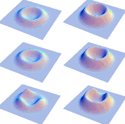
FIG. 4.: Spin down- (left column) and total (right column) densities of a six electron ring with $r_{s,1D}=2$, $C_{F}=7$, $\phi=0$, $S=0$ and impurity strengths (from the top) $V_{0}=0.0,~{}0.1,~{}0.5$. Increasing $V_{0}$ gradually localizes the electrons and reduces the density at the location of the impurity.

The spin, $S$, is zero in the ground state, see Fig.3. In this case, the density of both spin components is homogeneous and rotationally invariant for $V_{0}=0$ and $0.1$, whereas one can see that the electrons start to get localized at larger $V_{0}$. This localization is accompanied by the formation of a spin-density wave (SDW), with alternating spin up- and spin down electrons. We also see that the density at the impurity center decreases with increasing $V_{0}$. A more systematic analysis of this effect is presented in Fig.5, where we show the total electron density at ($x=R_{0}$, $y=0$) as function of impurity strength for the same ring at three different flux values, and also a more narrow ring with $C_{F}=16$, all normalized by the density at $V_{0}=0$. The curves roughly fall on top of each other, independent of $\phi$ and $C_{F}$ and seem to fall off exponentially as function of the impurity strength.

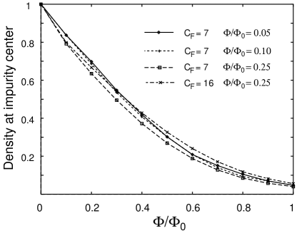
FIG. 5.: Density at impurity center vs. impurity strength for a set of six-electron rings with $r_{s,1D}=2$, $C_{F}=7$ and $\phi=0.05\phi_{0}$, $\phi=0.1\phi_{0}$ and $\phi=0.25\phi_{0}$, and also $C_{F}=16$, $\phi=0.25\phi_{0}$, all in the $S=0$ state and normalized by their densities at $V_{0}=0$. The shape of these curves is roughly independent of flux strength and of $C_{F}$.

Fig.6 shows an example of how the persistent current falls off with increasing impurity strength $V_{0}$ ($a=b=2$) in a six-electron ring ($r_{s,1D}=2$, $C_{F}=7$) in the $S=1$ state at $\phi=0.25\phi_{0}$. This choice of parameters, though not corresponding to the ground state (see Fig.3), is particularly convenient due to the large absolute value of the current, making numerical error less significant. We have checked that other (ground state) sets of parameters give qualitatively the same behavior. We note that the form of this curve, with a plateau at small $V_{0}$, followed by steeper fall-off, is very similar to the result by Cheung et al. [9], obtained by numerical diagonalization of an ideal one-dimensional ring with 20 electrons in the tight binding approximation.

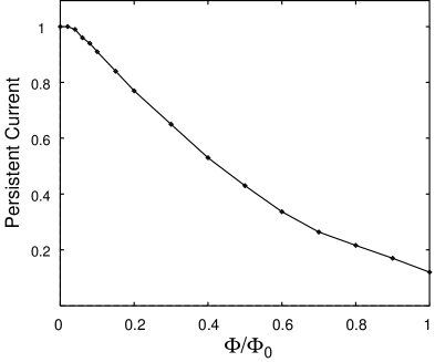
FIG. 6.: Persistent current vs. impurity strength for a six-electron ring in the $S=1$ state with $r_{s,1D}=2$, $C_{F}=7$ and $\phi=0.25\phi_{0}$.

Finally, we examine another effect which tends to localize the electrons in the ring: It turns out that making the ring more one-dimensional, i.e. increasing $C_{F}$ keeping everything else fixed, gradually localizes the electrons, creating a strong SDW along with a spatial modulation of the total charge density (CDW). This is illustrated in Fig.7 where we show density profiles of a six-electron ring with $r_{s,1D}=2$ at zero flux and without an impurity for three different values of $C_{F}$.

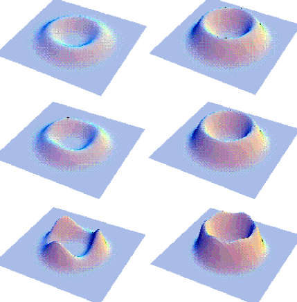
FIG. 7.: Spin down- (left column) and total (right column) densities of an impurity-free six electron ring with $r_{s,1D}=2$, $\phi=S=0$ and (from the top) $C_{F}=7,~{}8,~{}12$. Increasing $C_{F}$, i.e. narrowing the confining potential, gradually localizes the electrons.

Such localization and antiferromagnetic ordering of the electron spin in a quasi one-dimensional ring confinement was recently confirmed by exact diagonalization studies: the many-body spectra of quantum rings with up to 6 electrons could be described by a spin model combined with a rigid center-of mass rotation [31]. The stronger the ring confinement (i.e. the more narrow the quasi one-dimensional ring), or the lower the average particle density, the more pronounced are the effects of localization and formation of charge density waves in the internal structure of the many-body wave function.

One might expect that an impurity potential would “pin” a charge density wave in the ring, i.e. the persistent current of a ring with localized electrons should be reduced as compared to the non-localized case. We have examined the possibility of such a “pinning-depinning transition” by computing the persistent current at fixed impurity strength as a function of $C_{F}$. Fig.8 shows the result for several different values of the impurity strength $V_{0}$. We see that the current indeed decreases as the ring becomes more narrow; however, there is no “abrupt” transition since, as we have seen, localization happens gradually with increasing $C_{F}$.

FIG. 8.: Persistent current vs. $C_{F}$ for a six-electron ring with $S=0,~{}r_{s,1D}=2,~{}\phi=0.25\phi_{0}$ at various impurity strengths, $V_{0}=0.0,~{}0.3,~{}0.6,~{}0.9$ (from the top) and $a=2.5$, $b=0.5$.

Note the interesting scaling behavior suggested by Fig.8: The ratio between any two of the curves is just a constant, independent of $C_{F}$; in particular, the ratio $I(V_{0})/I(V_{0}=0)$ is independent of $C_{F}$ for any $V_{0}$. Also note that the persistent current decreases with increasing $C_{F}$ even in the zero impurity case, thus making no qualitative distinction between a “clean” and a “dirty” ring. This may again be due to the explicit symmetry breaking by the LSDA which, as we have discussed previously, in a sense mimics disorder even in the case $V_{0}=0$.

V Conclusion

The numerical analysis presented here demonstrates that the current-spin-density-functional formalism provides a suitable tool for describing the effects of Aharonov-Bohm phases and impurities in realistic quantum rings. In particular, we have shown that it reproduces the main qualitative features of the many-body spectra and persistent currents, taking into account the effects of interactions, spin and deviations from perfect one-dimensionality. Furthermore, we have shown that the persistent current in the ring may be suppressed by narrowing the confining potential at fixed impurity strength.

The main difference between this model and exact diagonalization results is that the LSDA introduces a breaking of the rotational symmetry in the ring even in the impurity-free case. One may hope that this is not a problem when describing experimentally realizable quantum rings, as a certain amount of disorder and non-perfect symmetry is expected to be present in any realistic system.

With the present experimental progress in fabricating and studying few-electron quantum rings, the methods described here may turn out useful for suggesting and describing future experiments.

ACKNOWLEDGEMENT: This work was financially supported by the Academy of Finland, the TMR programme of the European Community under contract ERBFMBICT972405, the “Bayerische Staatsministerium für Wissenschaft, Forschung und Kunst”, and the NORDITA Nordic project “Confined electronic systems”.

REFERENCES

- [1] J. M. Garcia, G. Medeiros-Ribeiro, K. Schmidt, T. Ngo, J. L. Feng, A. Lorke, J. Kotthaus, and P. M. Petroff, Appl. Phys. Lett. 71, 2014 (1997).
- [2] A. Lorke and R. J. Luyken, Physica B 256, 424 (1998).
- [3] A. Lorke, R. J. Luyken, A. O. Govorov, J. P. Kotthaus, J. M. Garcia, and P. M. Petroff preprint cond-mat/9908263.
- [4] Y. Aharonov and D. Bohm, Phys. Rev. 115, 485 (1959).
- [5] F. Hund, Ann. Phys. (Leipzig) 32, 102 (1938).
- [6] N. Byers and C. N. Yang, Phys. Rev. Lett. 7, 46 (1961).
- [7] F. Bloch, Phys. Rev. B 2, 109 (1972).
-
[8]
M. Büttiker, Y. Imry, and R. Landauer,
Phys. Lett. A 96, 365 (1983);
M. Büttiker, Phys. Rev. B 32, 1846 (1985). - [9] H.-F. Cheung, Y. Gefen, E. K. Riedel, and W.-H. Shih, Phys. Rev. B 37, 6050 (1988).
- [10] N. Yu and M. Fowler, Phys. Rev. B 45, 11795 (1992).
- [11] V. Ambegoakar and U. Eckern, Phys. Rev. Lett. 65, 381 (1990).
- [12] U. Eckern and A. Schmid, Europhys. Lett. 18, 457 (1992).
- [13] T. Chakraborty and P. Pietiläinen, Phys. Rev. B 50, 8460 (1994).
- [14] T. Chakraborty and P. Pietiläinen, Phys. Rev. B 52, 1932 (1995).
- [15] K. Niemelä, P. Pietiläinen, P. Hyvönen, and T. Chakraborty, Europhys. Lett. 36, 533 (1996).
- [16] A. Emperador, M. Barranco, E. Lipparini, M. Pi, and Ll. Serra, Phys. Rev. B 59, 15301 (1999).
- [17] A. Emperador, M. Pi, M. Barranco, and A. Lorke, preprint cond-mat/9911127.
- [18] L. P. Lévy , G. Dolan, J. Dunsmuir, and H. Bouchiat, Phys. Rev. Lett. 64, 2074 (1990).
- [19] V. Chandrasekar, R. A. Webb, M. J. Brady, M. B. Ketchen, W. J. Gallagher, and A. Kleinsasser, Phys. Rev. Lett. 67, 3578 (1991).
- [20] D. Mailly, C. Chapelier, and A. Benoit, Phys. Rev. Lett. 70, 2020 (1993).
- [21] G. Vignale and M. Rasolt, Phys. Rev. B 37, 10685 (1988).
- [22] M. Ferconi and G. Vignale, Phys. Rev. B 50, 14722 (1994).
- [23] O. Heinonen, M. I. Lubin, and M. D. Johnson, Phys. Rev. Lett. 75, 4110 (1995)
- [24] M. Ferconi, and G. Vignale, Phys. Rev. B 56, 12108 (1997).
- [25] O. Steffens, U. Rössler, and M. Suhrke, Europhys. Lett. 42, 529 (1998).
- [26] M. Pi, M. Barranco, A. Emperador, E. Lipparini, and Ll. Serra, Phys. Rev. B 57, 14783 (1998).
- [27] M. Koskinen, J. Kolehmainen, S. M. Reimann, J. Toivanen, and M. Manninen, Eur. J. Phys. D 9, 487 (1999).
- [28] S. M. Reimann, M. Koskinen, M. Manninen and B. Mottelson, Phys. Rev. Lett. 83, 3270 (1999).
- [29] J. Kolehmainen, S. M. Reimann, M. Koskinen, and M. Manninen, Eur. Phys. J. B 13, 731 (2000).
- [30] S. M. Reimann, M. Koskinen, and M. Manninen, Phys. Rev. b 59, 1613 (1999).
- [31] M. Koskinen, M. Manninen, B. Mottelson, and S. M. Reimann, preprint cond-mat/0004095.