Current driven switching of magnetic layers

Abstract

The switching of magnetic layers is studied under the action of a spin current in a ferromagnetic metal/non-magnetic metal/ferromagnetic metal spin valve. We find that the main contribution to the switching comes from the non-equilibrium exchange interaction between the ferromagnetic layers. This interaction defines the magnetic configuration of the layers with minimum energy and establishes the threshold for a critical switching current. Depending on the direction of the critical current, the interaction changes sign and a given magnetic configuration becomes unstable. To model the time dependence of the switching process, we derive a set of coupled Landau-Lifshitz equations for the ferromagnetic layers. Higher order terms in the non-equilibrium exchange coupling allow the system to evolve to its steady-state configuration.

. ]

I Introduction

The possibility of using the exchange field of a spin-polarized current to aid in switching of a magnetic layer is not only an intruiging prospect for future applications in the field of magneto-electronics but also a challenge with interesting physics. There is still a lot of ambiguity in the interpretation of the complex data of the recently observed switching of domains in spin valves [1] and tunnel junctions [2], of magnetic clusters [3] and layers [4], nonetheless, in Refs. [1, 3, 4] it has been argued that the switching occurs through relaxation of conduction electron spin-polarization to the local moments of the ferromagnetic layers as proposed by Slonczewski [5, 6].

In this work we introduce a different model for the switching, where the spin-polarization does not relax. The effect is that the spin current carries an exchange field that acts on the local moments of a layer and forces its magnetization to take the orientation of the spin-polarization of the conduction electrons.

In the conventional view one considers electrons flowing in the direction of the net current from, say, a “fixed” layer that has a large magnetic moment to a “free” layer that has a small magnetic moment which is easy to reorient (see Fig. 1). The effect on the free layer is indeed relatively small as the associated energy, which is of the Zeeman-type, is proportional to the product of the small moment of the free layer and the exchange field of the conduction electrons polarized by the fixed layer (refer to upper part of Fig. 2). However, this picture neglects the much larger, albeit counter intuitive, effect of spin-dependent reflection of electrons by the free layer, so that spin-polarized electrons move in the direction opposite to the net current and interact with the large magnetic moment of the fixed layer. The energy of this contribution is thus also much larger and of opposite sign (see lower part of Fig. 2).

Taken together, both contributions establish a strong non-equilibrium exchange interaction (NEXI) between layers [7]. The sign of this interaction is determined by the direction of the current; it does not oscillate and its range is controlled by the spin diffusion length of the conduction electrons [8, 9]. Therefore, the NEXI is a volume effect and exerts a torque (force) throughout the volume of the magnetic layers (leading to precession); it is the dominant mechanism that drives the system towards its switching threshold. Here, we describe a simple model that shows how the NEXI defines the magnetic configuration of the layers with minimum energy, while the relaxation of the conduction electron spin polarization provides a way for the system to evolve to its minimum energy configuration.

The rest of the paper is structured as follows. In Sec. II we introduce our model of a spin valve and give a brief derivation of the NEXI. To illustrate the switching mechanism of the spin valve, in Sec. III we derive a set of coupled Landau-Lifshitz equations for uniform magnetic dynamics, whose structure is similar to those of antiferromagnets or ferrimagnets; however with the important difference that they are current driven and the magnetic sublattices are replaced by the spatially separate magnetic layers. The following stability analysis in Sec. IV shows that depending on the direction of the current either the parallel or the antiparallel configuration becomes unstable beyond a critical current, so that, in principle, even an arbitrarily small amount of relaxation allows a switching of the magnetically “softer”, i.e. free, layer. Despite the simplicity of our model, quantitative estimates are in reasonable agreement with experiments. In Sec. V we introduce Gilbert damping to describe possible relaxation processes that allow the system to evolve over time to its minimum energy configuration, i.e. to switch. Finally, we compare our results to the models by Slonczewski [5, 6], and Berger [10] in Sec. VI and conclude in Sec. VII.

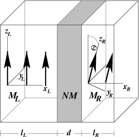
FIG. 1.: The geometry of a standard trilayer spin-valve; two planar ferromagnetic metal layers of thickness $l_{L(R)}$ and total magnetic moments ${\bf M}_{L(R)}$ at an angle $\Theta$ relative to each other are separated by a non-magnetic metal spacer NM of thickness $d$.

II Non-equilibrium exchange interaction (NEXI)

The geometry of our model system is a typical spin-valve structure shown in Fig. 1. It consists of two planar ferromagnetic metal layers of thickness $l_{L(R)}$ whose total magnetic moments ${\bf M}_{L(R)}$ are at an angle $\Theta$ relative to each other. The magnetic layers are separated by a non-magnetic metallic spacer NM of thickness $d$. A complete treatment of the magnetic dynamics of such a spin valve with a current in the perpendicular direction requires a simultaneous solution of the equation of motion for individual spins of the magnetic layers (see for example Ref. [11]), and equation of motion of the spin-polarized charge carriers [12].

To focus on the essential effects, the calculations are made on the simplest assumptions; we model the polycrystalline thin films as uniformly magnetized layers with uniaxial anisotropy in the plane of the layers. For clarity, we do not focus on the details that establish the equilibrium (zero current) coupling between magnetic layers; while the experiments [1] suggest that the equilibrium Ruderman-Kittel-Kasuya-Yosida (RKKY) coupling is negligible, the omission of the dipolar coupling between the layers (fringing fields) is probably a gross simplification of the physical picture. We treat the steady state non-equilibrium (constant current) situation in terms of the NEXI which can be written as a sum of quantum-interference and current driven terms; see for example Eqs. (2) and (3) in Ref. [8]. Although the first contribution to the coupling is finite at equilibrium, a.k.a. the RKKY interaction, it is a “surface” effect because it oscillates and scales as $1/d^{2}$ [13], therefore we will neglect it here as pointed out above. We posit that it is only the current driven term, which is a volume effect, that is responsible for the switching of the layers. Its decay is controlled by the spin diffusion length which is considerably longer than the typical thickness of spacer layers in metallic multilayers. Although our calculations are taken in the ballistic limit, they can be generalized to account for diffuse transport as will be pointed out in the text.

When a constant current is driven in the direction perpendicular to the plane of the magnetic layers, it becomes spin polarized. We define a spin current as:

$$\mbox{\boldmath$\Im$}(j_{L(R)}^{M})=j_{L(R)}^{M}{\bf n}_{L(R)},$$ (1)

whose polarization is along the unit vector of magnetization ${\bf n}_{L(R)}={\bf m}_{L(R)}/m_{L(R)}$ of the local moments, i.e. along the $z_{L(R)}$–axis in Fig. 1, which generates the polarization, and whose magnitude is

$${j}_{L(R)}^{M}=\frac{\mu_{B}}{e}\left({j}_{L(R)}^{\uparrow}-{j}_{L(R)}^{\downarrow}\right)=\frac{\mu_{B}}{e}\,{j}_{{\rm e}}\,\eta_{L(R)}.$$ (2)

We defined the electric charge and Bohr magneton as $e=-|e|$ and $\mu_{B}=|e|\hbar/(2m^{\ast}c)$, respectively; $m^{\ast}$ being the effective mass of the conduction electrons. Outside a magnetic layer the spin current decays within a distance of the spin-diffusion length $\lambda_{{\rm sf}}$, so that $\eta_{L(R)}$ is proportional to $\exp(-x/\lambda_{{\rm sf}})$ where $x$ is the distance away from the layer. The factor $\eta_{L(R)}$ describes the spin-dependent reflection (for diffuse transport this leads to the effect of spin accumulation and can be included in $\eta_{L(R)}$) and can vary between -1 and 1.

The NEXI comes then from the coupling of the spin current generated by the left layer ${\bf\mbox{\boldmath$\Im$}}(j_{L}^{M})$ interacting with the local moments in the right layer and vice versa. When we take as the direction of positive current from left to right, the coupling in linear response is:

$$E_{{\rm nexi}}^{{\rm eff}}=E_{R}(j_{L}^{M})+E_{L}(-j_{R}^{M}).$$ (3)

The local non-equilibrium coupling $E_{L(R)}$ is proportional to the scalar product in spin space of the spin current and the local moments, i.e. $E_{R}\propto{\bf\mbox{\boldmath$\Im$}}(j_{L}^{M})\cdot{\bf M}_{R}$ and similarly for $E_{L}$, where we averaged the spin-operators over the non-equilibrium statistical ensemble of the entire system, and have neglected spin-fluctuations [11]. From Eq. (1) follows, ${\bf\mbox{\boldmath$\Im$}}(-j_{L(R)}^{M})=-{\bf\mbox{\boldmath$\Im$}}(j_{L(R)}^{M})$, so that $E_{L}(-j_{R}^{M})=-E_{L}(j_{R}^{M})$, and Eq. (3) takes the form:

$$E_{{\rm nexi}}^{{\rm eff}} = E_{R}(j_{L}^{M})-E_{L}(j_{R}^{M})$$ (4)

$$= \mu_{R}\,{\bf h}_{LR}^{{\rm s-d}}\cdot{\bf M}_{R}-\mu_{L}\,{\bf h}_{RL}^{{\rm s-d}}\cdot{\bf M}_{L},$$ (5)

where ${\bf h}_{RL(LR)}^{{\rm s-d}}=J_{L(R)}{\bf\mbox{\boldmath$\Im$}}{(j_{R(L)}^{M})}/({v_{L(R)}^{F}}\mu_{L(R)}\mu_{B})$ are the local non-equilibrium exchange fields in the mean field approximation. Here $J_{L(R)}$ is the coupling constant between conduction electrons and local moments; $\mu_{L(R)}=g_{L(R)}\mu_{B}$, and $g_{L(R)}$ is the Landé factor in the respective layer. The preceding discussion can be visualized by Fig. 2. Another way of writing Eq. (5) is in terms of an effective Heisenberg coupling that depends on the current:

$$E_{{\rm nexi}}^{{\rm eff}} = \left(\mu_{R}\,\frac{{h}_{LR}^{{\rm s-d}}}{M_{L}}-\mu_{L}\,\frac{{h}_{RL}^{{\rm s-d}}}{M_{R}}\right){\bf M}_{L}\cdot{\bf M}_{R}$$ (6)

$$\equiv -J^{{\rm eff}}{\bf M}_{L}\cdot{\bf M}_{R}.$$ (7)

In Eqs. (5) and (7), respectively, we also introduced the simplifying assumption that the amount of spin polarization $\eta_{L(R)}$ does not depend on the angle $\Theta$ between the magnetic layers (see Fig. 1) and that there is no relaxation other than spin-diffusion. In fact the spin-polarized current of each layer depends on boundary condition to adjacent layers, e.g., as outlined in Ref. [14], so that $\eta_{L(R)}$ has to be calculated self-consistently from Eqs. (2) and (5), by taking into account the back effect of the coupling between the layers on the spin-polarization itself. A simple illustration of an approach which is self consistent in the current but not in energy can be given in the limit of diffusive transport by calculating the difference in energies for parallel and antiparallel configuration associated with the spin accumulation in the spin-valve. Using the picture developed in Ref. [14], one finds that for different layer thickness this energy contribution is non-vanishing. Details will be given elsewhere for a fully self-consistent calculation.

The form of Eq. (5) leads to some immediate consequences. If the system is symmetric in its magnetic properties, then, for the assumed linear response regime of the current, which is reasonably well satisfied in metallic multilayers even for high current densities, the two couplings $E_{L}$ and $E_{R}$ are equal and opposite, so that there is no non-equilibrium coupling between the layers. If, however, the magnetic properties or the thickness of the magnetic layers are dissimilar (in general, this would include non-uniform magnetization), the spatial symmetry of the system is broken and a current driven coupling between the layers exists. In particular, on reversing the current the interlayer coupling changes sign.

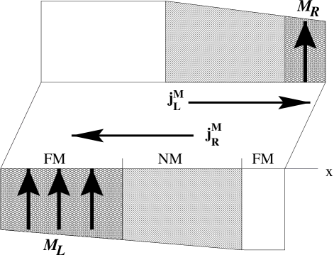
FIG. 2.: The figure shows the two contributions of the spin-current to the non-equilibrium exchange interaction (NEXI) given by the hatched regions: the forward contribution $j_{L}^{M}$ from the left ferromagnet and the reflected contribution $j_{R}^{M}$ from the right ferromagnet. The NEXI between the two ferromagnetic layers, as shown here for parallel configuration, is given by the difference of the double hatched regions which are proportional to $j_{L}^{M}M_{R}$ and $j_{R}^{M}M_{L}$, respectively. Only in certain limiting cases one of the contributions can be neglected.

III Equations of motion

To obtain the equation of motion for the magnetization of the spin valve, we follow the standard procedure and define an effective field [15],

$${\bf h}_{L(R)}^{{\rm eff}}={\bf h}_{L(R)}^{(i)}+\beta_{L(R)}{\bf n}_{L(R)}^{{\rm a}}\left({\bf m}_{L(R)}\cdot{\bf n}_{L(R)}^{{\rm a}}\right),$$ (8)

which is derived from the total energy of the system including the effects of uniaxial anisotropy, dipole-dipole interactions, and $E_{{\rm nexi}}^{{\rm eff}}$ of Eq. (5). The internal field (first term in Eqs. (8)) includes a contribution from the external field ${\bf h}^{{\rm(e)}}$, the spin current, and the magnetic dipole–dipole interaction which in a uniformly magnetized ellipsoid takes the form

$${\bf h}_{L}^{(i)} = {\bf h}^{(e)}+{\bf h}_{L}^{\rm nexi}-4\pi{\bar{N}}_{L}\cdot{\bf m}_{L},$$ (10)

$${\bf h}_{R}^{(i)} = {\bf h}^{(e)}+{\bf h}_{R}^{\rm nexi}-4\pi{\bar{N}}_{R}\cdot{\bf m}_{R},$$ (11)

where ${\bar{N}}_{L(R)}$ is the tensor of demagnetization factors, and

$${\bf h}_{L}^{\rm nexi} = \frac{J^{\rm eff}}{\mu_{L}}\,{\bf M}_{R}=\left({h}_{RL}^{{\rm s-d}}-h_{LR}^{{\rm s-d}}\,\frac{\mu_{R}}{\mu_{L}}\frac{M_{R}}{M_{L}}\right){\bf n}_{R},$$ (13)

$${\bf h}_{R}^{\rm nexi} = \frac{J^{\rm eff}}{\mu_{R}}\,{\bf M}_{L}=\left(h_{RL}^{{\rm s-d}}\,\frac{\mu_{L}}{\mu_{R}}\frac{M_{L}}{M_{R}}-{h}_{LR}^{{\rm s-d}}\right){\bf n}_{L},$$ (14)

are the effective non-equilibrium coupling fields between the layers induced by the spin-current, which vanish for identical layers. In general, when magnetic layers cannot be described by single domain particles, this symmetry condition does not hold due to the non-uniformity of the layers. Further, in such a case the coupling fields (III) will contain additional contributions from the fluctuation of the magnetization. The second term in Eqs. (8) is due to the uniaxial anisotropy, where $\beta_{L(R)}$ is the corresponding constant and ${\bf n}_{L(R)}^{{\rm a}}$ its in-plane unit vector. We would like to point out that the assumption of uniform magnetization means, in addition, that the effect of the induced magnetic field from the current, which leads to vortex formation, is small compared to the coupling field ${\bf h}^{{\rm nexi}}$ so that we can use the magnetostatic approximation in which ${\bf h}^{{\rm(e)}}$ is the field produced by currents in coils alone. The equations of motion are then given by

$$\frac{\partial{\bf M}_{L(R)}}{\partial t}=-\gamma_{L(R)}\left[{\bf M}_{L(R)}\times{\bf h}^{\rm eff}_{L(R)}\right]+{\bf R}_{L(R)},$$ (15)

where $\gamma_{L(R)}=g_{L(R)}\mu_{B}/\hbar>0$ are the gyro-magnetic ratios. The damping terms ${\bf R}_{L(R)}$ will be discussed in detail later.

Parenthetically, the solution of Eqs. (15) is closely related to solving the equations of motion for an antiferromagnet or ferrimagnet, where now an effective field of the exchange coupling does not act between sublattices but different layers. Therefore, due to the NEXI there exist long wavelength “acoustical” and “optical” modes wherein the magnetizations precess either in or out of phase. In an experimental set-up similar to the one described in Refs. [16, 17, 18], this would offer a direct possibility to measure the coupling between the magnetic layers as a function of applied current. The details will be presented elsewhere.

IV Critical current

So far we have derived the equations of motion for two coupled magnetic particles. The solution of the equations requires to divide the problem into a stationary one, which we shall consider first, and time-dependent one. In other words, before studying any form of dynamic behaviour of the magnetization, one must first determine the steady-state, i.e., the orientations of the magnetizations in the absence of time dependent driving fields. This orientation depends on the current. In combination with Eqs. (15), we obtain the equilibrium (steady state or constant current) configuration of the moments from the conditions:

$${\bf h}_{L(R)}^{\rm eff}|_{0}\times{\bf M}_{L(R)}=0,$$ (16)

which are independent of the time-dependent damping term and where also the effective field ${\bf h}_{L(R)}^{\rm eff}|_{0}$ does not depend on time. These conditions have to be satisfied simultaneously for both magnetic layers. For many applications, there exists an interesting limiting case where the thickness and anisotropy of one of the layers is very large, termed the fixed layer, so that one can assume, for example, ${\bf n}_{L}={\bf n}_{L}^{{\rm a}}$. In other words, the back effect of the right layer, termed the free layer, will be negligible on the orientation of the left layer but not on their mutual orientation. To be more explicit, we study the steady state of this example in more detail.

Instead of applying the conditions in Eqs. (16), a more straightforward method is to minimize the total energy of the system. By using the notation we introduced in Fig. 1 and assuming that the geometry of the film constrains the magnetization to be in the plane of the layer, the total energy of the system, in the absence of an external magnetic field, depends only on the angle $\Theta$ between the magnetic moments of the left and right layer:

$$E(\Theta)= - \frac{\beta_{L}}{2}m_{L}M_{L}-\frac{\beta_{R}}{2}m_{R}M_{R}\cos^{2}(\Theta-\Theta_{R}^{{\rm a}})$$ (17)

$$- h_{R}^{{\rm nexi}}M_{R}\cos\Theta,$$ (18)

where $\Theta_{R}^{{\rm a}}$ is the angle between the easy axis of the right layer with $z_{L}$, and

$$h_{R}^{{\rm nexi}}=h_{RL}^{{\rm s-d}}\,\frac{M_{L}}{M_{R}}-h_{LR}^{{\rm s-d}}$$ (19)

is the effective field value of the NEXI on the right layer of Eq. (14) with $\mu_{L}=\mu_{R}\equiv\mu$. From Eq. (19) it follows that for asymmetric magnetic layers a coupling exists which will be dominated by the spin current generated by the right layer if the total magnetic moment of the left layer exceeds that of the right one, i.e. $M_{L}>M_{R}$. In recent experiments one of the magnetic layers is chosen to be much thicker [1] so that $M_{L}\gg M_{R}$, and in the following discussion we shall assume this is the case. From the discussion after Eq.(1) it should be noted that $h_{LR(RL)}^{{\rm s-d}}$ is proportional to $\lambda_{{\rm sf}}/l_{R(L)}$ for $l_{L(R)}>\lambda_{{\rm sf}}$ inasmuch as $j_{L(R)}^{M}$ is limited by the spin diffusion length $\lambda_{{\rm sf}}$.

It is insightful to express the proportionality between the field $h_{R}^{{\rm nexi}}$ in Eq. (19) and the current density which generated it by the following relation:

$$\Lambda_{R}^{{\rm nexi}}\equiv\frac{h_{R}^{{\rm nexi}}}{j_{e}} = \frac{1}{\mu\,e}\left(\frac{J_{L}\eta_{R}}{v_{L}^{F}}\frac{M_{L}}{M_{R}}-\frac{J_{R}\eta_{L}}{v_{R}^{F}}\right)$$ (21)

$$\approx \frac{2\,m^{\ast}}{e}\frac{\eta_{L}\eta_{R}}{m_{R}}\left(v_{L}^{F}\frac{l_{L}}{l_{R}}-v_{R}^{F}\right).$$ (22)

Eq. (22) holds if we assume that the polarizations are the Pauli factors $\eta_{L(R)}=J_{L(R)}m_{L(R)}/(4\,\varepsilon_{F}^{L(R)}\mu)$, and $\varepsilon_{F}^{L(R)}$ the Fermi energies. One can, then, rewrite Eq. (19) as:

$$h_{R}^{{\rm nexi}}=\Lambda_{R}^{{\rm nexi}}j_{e}.$$ (23)

In other words, $h_{R}^{{\rm nexi}}$ plays the role of an exchange biasing field on the right layer generated by the current through the system. To get a better understanding, we give a rough estimate to the magnitude of $\Lambda_{R}^{{\rm nexi}}$. If we assume a magnetization for Co of $m_{R}=1.42\times 10^{6}$ A/m, a Fermi velocity of about 1.5$\times$10⁶ m/s, the layer thickness ratio $(l_{L}-l_{R})/l_{R}$=3, and use the free electron mass in Eq. (22), the only undetermined parameter is $\eta_{L(R)}$. Taking the hypothetical case that the amount of spin-polarization is the same throughout the system as in the ferromagnetic layer, we estimate for Co with $\eta=38$% $\Lambda_{R}^{{\rm nexi}}$ to be approximately 5$\times 10^{-5}$ m, which amounts to $1/\Lambda_{R}^{{\rm nexi}}\approx 0.02$ mA/kOe. The latter is about an order of magnitude lower than the value measured in the experiments on Co/Cu/Co pillars [4]. Therefore, our estimate for $\Lambda_{R}^{{\rm nexi}}$ derived for perfect spin polarization can be seen as an upper threshold for the proportionality between biasing field and current. Realistic estimates are obtained by adjusting the value for $\eta_{L(R)}$ taking spin-diffusion, spin-dependent reflection at the interfaces, and the resistance of the layers into account [7, 14]. Then for $\eta=10$% [19], we obtain direct agreement with experiments $1/\Lambda_{R}^{{\rm nexi}}\approx 0.29$ mA/kOe [4].

Having introduced the effective field $h_{R}^{{\rm nexi}}$ of the NEXI, we realize from the form of Eq. (18) that finding the switching threshold of the right layer (free layer) can be treated as if the layer were a single magnetic domain in an external magnetic field. The equilibrium direction of the magnetization of the right layer (free layer) is then obtained by the extremum energy condition $(\partial E/\partial\Theta)=0$. In addition, for the equilibrium to be stable (unstable) the following relation must hold: $(\partial^{2}E/\partial\Theta^{2})>(<)$ $0$. At $(\partial^{2}E/\partial\Theta^{2})=0$ the model predicts a transition from a gradual rotation of ${\bf n}_{R}$ to a sudden switching towards the direction of ${\bf n}_{L}^{{\rm a}}$, i.e. an irreversible magnetization rotation, which determines the critical coupling field $h_{{\rm c}}^{{\rm nexi}}$. Since we have two conditions and the two unknown variables $\Theta$ and $h_{{\rm c}}^{{\rm nexi}}$, we can eliminate $\Theta$ and derive an expression for the critical coupling field $h_{{\rm c}}^{{\rm nexi}}$ obtained from the following relation (refer to Ref. [20] for the details of the derivation):

$$\sin 2\Theta_{R}^{{\rm a}}=\frac{1}{y^{2}}\left(\frac{4-y^{2}}{3}\right)^{3/2},$$ (24)

where $y=-2h_{{\rm c}}^{{\rm nexi}}/(\beta_{R}m_{R}^{0})$. From Eq. (24) we find that the critical field is maximum at $\Theta_{R}^{{\rm a}}=0$ and $\pi/2$, where, $h_{{\rm c}}^{{\rm nexi}}=-\beta_{R}m_{R}^{0}$, and minimum at $\Theta_{R}^{{\rm a}}=\pi/4$ when $h_{{\rm c}}^{{\rm nexi}}=-\beta_{R}m_{R}^{0}/2$. For a parallel orientation of the uniaxial anisotropies between the layers $\Theta_{R}^{{\rm a}}=0$ this translates together with Eqs. (2) and (19) to the following condition for a spin current induced switching:

$$-j_{{\rm e}}^{{\rm c}} \geq \frac{2\,K_{R}^{\rm u}}{\Lambda_{R}m_{R}}$$ (26)

$$\approx \frac{e}{m^{\ast}}\frac{K_{R}^{{\rm u}}}{\eta_{L}\eta_{R}}\frac{l_{R}}{l_{L}v_{L}^{F}-l_{R}v_{R}^{F}}$$ (27)

$$\approx \frac{e}{m^{\ast}}\frac{K_{R}^{{\rm u}}}{v_{L}^{F}}\frac{1}{\eta_{L}\eta_{R}}\frac{l_{R}}{l_{L}},$$ (28)

where $j_{{\rm e}}^{{\rm c}}$ is the critical current density, and $K_{R}^{{\rm u}}=\beta_{R}\,m_{R}^{2}/2$ the standard expression for the uniaxial anisotropy constant [21]. Eq. (27) holds if we assume again that the polarizations are the Pauli factors, and Eq. (28) is applicable when $M_{L}\gg M_{R}$. From Eq. (28) it becomes clear that the switching threshold is determined by the coupling of the spin current generated in the right layer (free layer) to the magnetization in the left layer (fixed layer); it would be inappropriate to replace the left layer in the problem by a simple spin-polarized current source in the switching experiments [1]. On the contrary, Eqs. (26) and (27) show that for almost identical layers the critical current becomes very large as the denominator tends to zero, so that only transient processes are relevant and, indeed, switching has not been observed [22]. Since $\eta_{L}\eta_{R}$ is a measure of the coupling strength, the critical current $j_{{\rm e}}^{{\rm c}}$ is thus inversely proportional to the coupling of the free layer to the fixed layer, so that a strong coupling reduces $j_{{\rm e}}^{{\rm c}}$; on the other hand, a high value of anisotropy $K_{R}^{{\rm u}}$ will increase $j_{{\rm e}}^{{\rm c}}$. More generally, $j_{{\rm e}}^{{\rm c}}$ is proportional not only to the uniaxial anisotropy but to whatever constrains the local moments; for example $j_{{\rm e}}^{{\rm c}}$ will also be strongly influenced by the dipolar coupling between layers and quantum interference (RKKY) contributions to the interlayer exchange coupling. Although $K_{R}^{{\rm u}}$ certainly cannot capture the details of the switching, it yields a simple analytical solution that provides the intuitive picture that current driven switching can be treated as a single magnetic particle in the current driven exchange field $h_{R}^{{\rm nexi}}$. This description is particularly appealing as it allows one to treat generalizations of our model similar to those known from magnetic recording [20].

We chose $\Theta=0$ to be the parallel alignment of the magnetic moments for zero current and the direction of current from left to right which led to a negative sign in front of $h_{R}^{{\rm nexi}}$ in Eq. (18). Thus, the parallel configuration is only preferable if $h_{R}^{{\rm nexi}}$ is positive. Having related $h_{R}^{{\rm nexi}}$ to the current (refer to Eqs. (2) and (19)), the system becomes then unstable for a sufficient negative current (24) which forces the spin valve to switch to an antiparallel configuration. Similarly, starting from an antiparallel orientation, a positive current switches the spin valve to parallel. We can also give a rough estimate to the magnitude of required critical current densities. Using again the same data as before of Ref. [4] and an uniaxial anisotropy for Co of $K_{R}^{\rm u}=1.5\times 10^{4}$ J/m³, we estimate the lower limit of the critical current for perfect spin polarization in Eq. (27) to be approximately 0.4$\times$10⁷ A/cm²; this is more than an order of magnitude lower than what is needed for the actual switching observed in the experiments [4], consistent with our limiting estimate on $1/\Lambda_{R}^{{\rm nexi}}$. Using, however, the more realistic value $\eta=10$% we obtain a critical current of 0.6$\times$10⁸ A/cm² in good agreement with the experiments [4].

V Relaxation processes

The conditions for a critical current were obtained from the solution of the stationary problem. To describe the dynamics of the switching process, one has to solve the time-dependent problem. In addition, we have to introduce relaxation, because without it the right layer would only precess but never switch, no matter how strong the current would be. However, when the steady state configuration is unstable, even the slightest relaxation is sufficient for the magnetization to switch. A wealth of possible relaxation mechanisms arises from the non-uniform motion of the magnetic moments, which we have excluded here by making the assumption that the layers can be treated as two coupled uniformly magnetized particles; also we neglected the back effect of the NEXI on the spin polarization $\eta_{L(R)}$ which reduces the coupling. An important mechanism for relaxation is the transfer of angular momentum from the conduction electrons to the local moments as discussed by Slonczewski [5, 6] and Berger [10].

Although it is possible to derive this contribution by systematically taking the perturbation expansion of the $s$–$d$ Hamiltonian to third order, here we will simply posit it by introducing a phenomenological Gilbert damping in Eqs. (15):

$${\bf R}_{L(R)}=\frac{\alpha_{L(R)}}{M_{L(R)}}\;{\bf M}_{L(R)}\times\frac{\partial{\bf M}_{L(R)}}{\partial t},$$ (29)

where $\alpha_{L(R)}$ is a dimensionless damping parameter that depends on the current and on the layer thickness. We concentrate only on the part of $\partial{\bf M}_{L(R)}/\partial t$ due to the NEXI; all other contributions follow in analogy from the expression of the effective field (8). If we substitute in Eqs. (15) $\gamma_{R}$ with $\gamma_{R}^{\ast}=\gamma_{R}/(1+\alpha_{R})$ we can transform Eq. (29) into one of the following forms:

$${\bf R}_{R}^{{\rm nexi}} = -\frac{\omega_{R}}{M_{R}M_{L}}\;{\bf M}_{R}\times\left({\bf M}_{R}\times{\bf M}_{L}\right)$$ (31)

$$= -\omega_{R}\left({\bf m}_{R}\cos\Theta-\chi_{R}^{0}{\bf h}_{R}^{{\rm nexi}}\right)V_{R},$$ (32)

where $\omega_{R}=\alpha_{R}\gamma_{R}^{\ast}h_{R}^{{\rm nexi}}$ is the damping frequency due to the NEXI, $\chi_{R}^{0}=m_{R}/h_{R}^{{\rm nexi}}$ the respective susceptibility, and $V_{R}$ the volume of the layer. The first way of writing the relaxation resembles the effect of the conduction electron spin relaxation of Refs. [5, 6]. The result therein, that the surface torques of both layers impel ${\bf m}_{L}$ and ${\bf m}_{R}$ to rotate in the same direction in the plane of the layer, applies also to our case as can be seen from Eqs. (10) and (29). However, our conclusions are different. With reference to Eq. (15), we note that the NEXI, being the leading order contribution to the switching, determines the precession so that the effect of ${\bf R}_{L(R)}^{{\rm nexi}}$ is to reduce the coupling and thus minimize the energy in Eq. (18). This is demonstrated by the second way of writing Eq. (29) which leads to the interpretation that ${\bf m}_{R}$ relaxes towards the non-equilibrium exchange field ${\bf h}_{R}^{{\rm nexi}}$ whose orientation is determined by that of the conduction electron spin polarization which is controlled by ${\bf m}_{L}$ and the direction of the current. In other words, if the system becomes unstable, ${\bf R}_{R}^{\rm nexi}$ dominates all other contribution in the Gilbert damping, so that ${\bf R}_{R}^{\rm nexi}$ drives the system to its new minimum energy configuration, i.e. towards the direction of ${\bf h}_{R}^{{\rm nexi}}$. This reasoning is analogous to what happens to a single magnetic particle in an externally applied switching field.

Finally, the way in which we introduced the phenomenological damping, relates the time for the total magnetization to reorient to the relaxation frequency $\omega_{R}$; the switching motion becomes more viscous as $\omega_{R}$ becomes large. This coincides with the common notion that the switching time is expected to be fastest for a moderate value of $\omega_{R}$, and might allow one to use Eqs. (15) despite their simplicity to model current driven switching dynamics in more realistic systems.

VI Discussion

We have shown that in order to describe current driven switching of magnetic layers in sub-micron sized spin-valve structures, it is in general necessary to include the non-equilibrium coupling between layers. Only in cases where the system is in linear response and the magnetic layers are identical, or the spin-diffusion length very short, one can neglect its contribution. The assumptions taken in our model are that of two single domain particles with an uniaxial anisotropy and a non-equilibrium coupling mediated by the spin-current and a local $s$–$d$ exchange interaction. These are certainly gross simplifications of the physical situation, however, they give quantitative agreement with experiments for a reasonable choice of the magnetic parameters.

In making comparison with Slonczewski’s model [5, 6], it should be noted that we make a different set of assumptions. In his case the NEXI was neglected and the system was reduced to consisting of a magnetic layer, that serves as a constant source of spin-polarized electrons, and a single domain particle which acts as a perfect spin filter, i.e. that all majority spins are transmitted whereas all minority spins are reflected. The assumption of spin-filtering distinguishes Slonczewski’s theory from that of Berger [10], who invokes inelastic spin-flip scattering. However, only inelastic spin-flip scattering allows for multiple spin-wave excitations that can reorient the axis of quantization in a magnetic layer and serves as a different type of switching mechanism in the limit of short spin-diffusion length, as will be shown further down in the text.

Spin-filtering, which we termed spin-dependent reflection, gives rise to interlayer coupling. It is non-dissipative to the leading order in the coupling which is described by the NEXI. Only the next order term in the interlayer coupling is proportional to Eqs. (29). By neglecting the term in leading order, Slonczewski finds only terms similar to Eq. (31) as the sole origin of multiple spin-wave excitations as predicted by Berger [23]. Our model produces the opposite effect: the precession of ${\bf m}_{R}$ is damped and relaxes towards the non-equilibrium exchange field ${\bf h}_{R}^{\rm nexi}$. It is also not surprising that after fitting the phenomenological damping parameter $\alpha_{G}$ [24] and adjusting $\eta$ to 10% [19], which coincides with our estimate, a good quantitative agreement with experiments is reached; the competition between the different damping terms ${\bf R}_{R}$ just reflects the competition between the different effective field contributions ${\bf h}^{\rm eff}_{R}$ (8) in the Landau-Lifshitz equation (15).

Nevertheless, Slonczewski’s theory is insightful in that it can describe spin-wave instabilities and shows how switching can occur due to inelastic spin-flip scattering at a multilayer interface after adaptation according to Berger [10]. To understand how such a switching mechanism is in principle possible, one has to consider first the creation of spin-waves in magnetic multilayers which were initially observed in point contact measurements of Co/Cu multilayers above a critical current [22]. As pointed out before, at the root of this phenomena lies a relaxation mechanism between conduction electrons and local moments due to spin-flip scattering. When a current flows from a non-magnetic metal layer to a ferromagnetic one, its distribution over spin-up and spin-down currents has to change. Given that most scattering events will conserve the current in each spin-subband, a difference in “chemical potentials” appears on the scale of the spin-diffusion length away from the interfaces [25] which leads to the effect of spin accumulation [14]. The critical current density for spin-wave emission is reached when the difference in “chemical potentials” of the spin subbands equals the energy of a spin wave $\Delta\mu=\mu_{\downarrow}-\mu_{\uparrow}=\hbar\omega$, so that in a spin-flip transition of a conduction electron the energy is conserved [10]. In this way magnetic moment is transferred to the system of localized spins at the non-magnetic/ferromagnetic metal interface as the conduction electron spin polarization changes.

For spin wave emission a second ferromagnetic layer (e.g. the left layer in Fig. 1) is not necessarily required as demonstrated in Fig. 2E of Ref. [1]. As long as only linear spin-waves are excited, the transfer of magnetic moment to the local moments leads just to a reduction of magnetization [26], similar to increasing the temperature. The reorientation of the axis of quantization of the ferromagnet, i.e. the switching, takes place only if non-linear spin-waves are created [21] which occurs for much higher current densities. For currents below a critical value the relaxation mechanism between the conduction electrons and the local moments allows only for a damping of already existing spin-waves [10], similar as in Sec. V.

Since switching seems to occur for current densities well below the critical value for spin-wave excitations, this mechanism is insufficient to lie at the origin of the switching. In particular for Co/Cu/Co spin valves, the data allows us to separate the hysteretic switching from the spin-wave excitations (refer to Fig. 2 in Ref. [1]); as mentioned earlier a spin-wave instability is observed already for an initially unpolarized current. This figure also shows clearly that the domains are reversed well before the onset of spin-wave instabilities and at current densities where transport yields more or less ohmic behaviour. Thus, experiments seem to provide evidence that the excitation of spin waves by the spin current is preceded by the switching process [1, 4] and, therefore, confirm our model for the switching based on the NEXI.

VII Conclusion

In conclusion, we showed that the current driven coupling provides the dominant energy term that promotes the switching of the magnetization of the layers in spin-valves [1, 4]. We pointed out the differences to the interpretation that the switching comes about by creating multiple spin-wave excitations due to inelastic spin-flip scattering which have to overcome only other forms of relaxation in the system.

An interesting test of our model is to compare an asymmetric structure, such as Co/Cu/Py, with a symmetric one, such as Co/Cu/Py/Cu/Co. One could also separate the effect of spin-wave excitations, i.e. $\Delta\mu=\hbar\omega$, for large currents from the switching, if one would apply an external field $h^{(e)}$ to the spin valve that is much stronger than $h_{R}^{{\rm nexi}}$ given in Eq. (19). On the other hand, interesting effects are expected to be observed in the region where $h_{R}^{{\rm nexi}}$ and $h^{(e)}$ are comparable; in this case much of the magnetic response of the spin-valve is due to non-uniformity of the magnetization of the layers which we neglected here.

We are indepted to Peter M. Levy for many stimulating discussions and helpful comments and would like to thank Roger H. Koch for the interest in our work. We are also grateful to John C. Slonczewski and Jonathan Z. Sun for communication of results prior to publication. This work was supported by the Defense Advanced Research Projects Agency and Office of Naval Research (Grant No. N00014-96-1-1207 and Contract No. MDA972-99-C-0009), and NATO (Grant Ref. No. PST.CLG 975312). P.E.Z. wishes to acknowledge the RFBR (Grant No. 00-02-16384).

REFERENCES

- [1] E. B. Myers et al., Science 285, 867 (1999).
- [2] C. Heide et al., J. Appl. Phys. 87, 5221 (2000).
- [3] J. Z. Sun, J. Magn. Magn. Mater. 202, 157 (1999).
- [4] J. A. Katine et al., Phys. Rev. Lett. 84, 3149 (2000).
- [5] J. C. Slonczewski, J. Magn. Magn. Mater. 159, L1 (1996).
- [6] J. C. Slonczewski, J. Magn. Magn. Mater. 195, L261 (1999).
- [7] C. Heide, R. J. Elliott, and N. S. Wingreen, Phys. Rev. B 59, 4287 (1999).
- [8] C. Heide and R. J. Elliott, Europhys. Lett. 50, 271 (2000).
- [9] Although in Ref. [7, 8, 13] the nonequilibrium exchange interaction was calculated for magnetic tunnel junctions, the general results can be applied readily to the case of metallic multilayers.
- [10] L. Berger, Phys. Rev. B 54, 9353 (1996).
- [11] C. Heide and P. E. Zilberman, Phys. Rev. B 60, 14756 (1999).
- [12] This simplified picture uses the notion that transition metals are reasonably well described by the – model; an assumption which holds only well within a phenomenological treatment of the coupling.
- [13] N. F. Schwabe, R. J. Elliott, and N. S. Wingreen, Phys. Rev. B 54, 12953 (1996).
- [14] T. Valet and A. Fert, Phys. Rev. B 48, 7099 (1993).
- [15] A. I. Akhieser, V. G. Baryakhtar, and S. V. Peletminskii, Spinovye Volny (Nauka, Moscow, 1967).
- [16] P. Grünberg et al., Phys. Rev. Lett. 57, 2442 (1986).
- [17] J. J. Krebs, P. Lubitz, A. Chaiken, and G. A. Prinz, Phys. Rev. Lett. 63, 1645 (1989).
- [18] B. Heinrich et al., Phys. Rev. Lett. 64, 673 (1990).
- [19] J. Z. Sun, (2000), to be published.
- [20] S. Chikazumi, Physics of Magnetism (John Wiley & Sons, Inc., New York, London, Sydney, 1964).
- [21] A. G. Gurevich and G. A. Melkov, Magnetization Oscillations and Waves (CRC Press, Boca Raton, 1996), p. 39.
- [22] M. Tsoi et al., Phys. Rev. Lett. 80, 4281 (1998).
- [23] It is interesting to note that in one of the first papers on current induced effects in magnetic multilayer systems by Slonczewski [27], the effect of the current on what is termed therein conservative exchange coupling was not considered.
- [24] J. C. Slonczewski, Paper L-4 presented at Frontiers in Magnetism Conference in Stockholm, Sweden August 12–15 (1999).
- [25] P. C. van Son, H. van Kempen, and P. Wyder, Phys. Rev. Lett. 58, 2271 (1987).
- [26] S. J. C. H. Theeuwen et al., Appl. Phys. Lett. 75, 3677 (1999).
- [27] J. C. Slonczewski, Phys. Rev. B 39, 6995 (1989).