Formation of Pairing Fields in Resonantly Coupled Atomic and Molecular Bose-Einstein Condensates

Abstract

In this paper, we show that pair-correlations may play an important role in the quantum statistical properties of a Bose-Einstein condensed gas composed of an atomic field resonantly coupled with a corresponding field of molecular dimers. Specifically, pair-correlations in this system can dramatically modify the coherent and incoherent transfer between the atomic and molecular fields.

PACS number(s): 32.80.Pj, 03.75.Fi

In quantum field theory, superfluidity and long-range order are usually identified with a complex-valued order parameter defined as the expectation value of the field operator. In the case of a dilute Bose gas, the evolution of the order parameter is given in the mean-field approximation by the well-known Gross-Pitaevskii equation. Recently, this equation has been extensively applied to studies of the zero-temperature collective behavior of metal-alkali Bose-Einstein condensates confined in magnetic traps [1]. Quantitative agreement has been found between theory and experiment on a wide range of distinct phenomena (e.g. Refs. [2, 3]).

Although identical in form to a non-linear Schrödinger equation, it is notable that the Gross-Pitaevskii equation does not by itself describe the full evolution of the quantum state. In general, a complete description requires knowledge of the evolution of a hierarchy of correlation functions, and not just the evolution of the expectation value of the field. In particular, in low temperature systems, it is well known that pairing fields associated with two-particle correlations can play an important role. In a quantum degenerate Fermi gas, pairing may radically alter the equilibrium properties, giving rise to superfluidity in ³He and superconductivity in electron systems. Correlations can also be important in Bose systems. For example, squeezed states of light—formed when photons are generated in pairs in nonlinear media—have been studied extensively in the subject of quantum optics [4].

In this paper, we investigate the role of pair-correlations on the macroscopic dynamics of a dilute Bose-Einstein condensate composed of atoms and molecules which are resonantly coupled [5, 6, 7, 8]. Such a coupling may be generated experimentally [9, 10] by tuning the strength of an external magnetic field in the proximity of a Feshbach resonance (see Fig. 1). Two parameters characterize the Feshbach resonance: (i) the energy mismatch $\epsilon$ between the bound state and the zero energy edge of the continuum states for the colliding atom pair, and (ii) the inverse lifetime $\kappa$ of the bound state. As an alternative, photoassociation may be used to directly generate the resonant coupling [11, 12]. In photoassociation, a two-photon Raman transition is used to couple the atomic continuum states and a specific bound molecular level. In that case $\epsilon$ represents the detuning energy of the Raman lasers from the atom-molecule transition, and $\kappa$ denotes the two-photon Rabi frequency proportional to the laser intensities and to the usual overlap integrals.

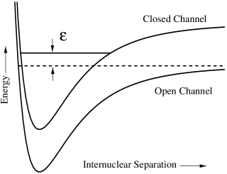
FIG. 1.: Feshbach resonance. Atoms collide with relative kinetic energy near zero as indicated by the dotted line. This energy is quasi-degenerate with a bound state in a closed channel potential. Typically, $\epsilon$ can be tuned experimentally by changing the magnitude of an external magnetic field.

An effective Hamiltonian for this coupled atom-molecule system may be written as

$$\hat{H} = \int d^{3}\mbox{\boldmath$x$}\,\hat{\psi}^{{\dagger}}_{a}(\mbox{\boldmath$x$})H_{a}(\mbox{\boldmath$x$})\hat{\psi}_{a}(\mbox{\boldmath$x$})+\hat{\psi}^{{\dagger}}_{m}(\mbox{\boldmath$x$})H_{m}(\mbox{\boldmath$x$})\hat{\psi}_{m}(\mbox{\boldmath$x$})$$ (5)

$${}+{U_{\rm aa}\over 2}\int d^{3}\mbox{\boldmath$x$}\,\hat{\psi}^{{\dagger}}_{a}(\mbox{\boldmath$x$})\hat{\psi}^{{\dagger}}_{a}(\mbox{\boldmath$x$})\hat{\psi}_{a}(\mbox{\boldmath$x$})\hat{\psi}_{a}(\mbox{\boldmath$x$})$$

$${}+U_{\rm am}\int d^{3}\mbox{\boldmath$x$}\,\hat{\psi}^{{\dagger}}_{a}(\mbox{\boldmath$x$})\hat{\psi}^{{\dagger}}_{m}(\mbox{\boldmath$x$})\hat{\psi}_{m}(\mbox{\boldmath$x$})\hat{\psi}_{a}(\mbox{\boldmath$x$})$$

$${}+{U_{\rm mm}\over 2}\int d^{3}\mbox{\boldmath$x$}\,\hat{\psi}^{{\dagger}}_{m}(\mbox{\boldmath$x$})\hat{\psi}^{{\dagger}}_{m}(\mbox{\boldmath$x$})\hat{\psi}_{m}(\mbox{\boldmath$x$})\hat{\psi}_{m}(\mbox{\boldmath$x$})$$

$${}+{g\over 2}\int d^{3}\mbox{\boldmath$x$}\,\hat{\psi}^{{\dagger}}_{m}(\mbox{\boldmath$x$})\hat{\psi}_{a}(\mbox{\boldmath$x$})\hat{\psi}_{a}(\mbox{\boldmath$x$})+\mbox{h.c.}\,,$$

where $\hat{\psi}_{a}(\mbox{\boldmath$x$})$ and $\hat{\psi}_{m}(\mbox{\boldmath$x$})$ are bosonic field operators which annihilate an atom or molecule respectively at coordinate $x$. Atomic binary collisions are characterized by the mean-field energy per unit density, $U_{\rm aa}=4\pi\hbar^{2}a/m$, where $m$ is the atomic mass, and $a$ is the scattering length for atom-atom collisions. Equivalent definitions apply for $U_{\rm am}$ and $U_{\rm mm}$ corresponding to atom-molecule collisions and molecule-molecule collisions. The process of inter-conversion of atom pairs into molecules is characterized by $g=\sqrt{\kappa\,U_{\rm aa}}$ [5]. The free Hamiltonians are

$$H_{a}(\mbox{\boldmath$x$}) = -{\hbar^{2}\over{2m}}\nabla^{2}_{\mbox{\boldmath$\scriptstyle x$}}+V_{a}(\mbox{\boldmath$x$})-\mu_{a}$$ (6)

$$H_{m}(\mbox{\boldmath$x$}) = -{\hbar^{2}\over{4m}}\nabla^{2}_{\mbox{\boldmath$\scriptstyle x$}}+V_{m}(\mbox{\boldmath$x$})-\mu_{m}\,,$$ (7)

where we include $V_{a}(\mbox{\boldmath$x$})$ and $V_{m}(\mbox{\boldmath$x$})$ for generality to allow for the possibility of external potentials. The chemical potentials of the atomic and molecular fields are denoted by $\mu_{a}$ and $\mu_{m}$ respectively, such that $\epsilon=\mu_{m}-2\mu_{a}$.

We solve for the evolution of the fields, assuming the principle of attenuation of many-particle correlations in the dilute gas. That is, we find the expectation value of the Heisenberg equations for $\hat{\psi}_{a}(\mbox{\boldmath$x$})$ and $\hat{\psi}_{m}(\mbox{\boldmath$x$})$ and separate explicitly the mean values of the field operators

$$\phi_{a}(\mbox{\boldmath$x$}) = \langle{\hat{\psi}_{a}(\mbox{\boldmath$x$})}\rangle$$ (8)

$$\phi_{m}(\mbox{\boldmath$x$}) = \langle{\hat{\psi}_{m}(\mbox{\boldmath$x$})}\rangle$$ (9)

from their zero-mean fluctuating components

$$\hat{\chi}_{a}(\mbox{\boldmath$x$}) = \hat{\psi}_{a}(\mbox{\boldmath$x$})-\phi_{a}(\mbox{\boldmath$x$})$$ (10)

$$\hat{\chi}_{m}(\mbox{\boldmath$x$}) = \hat{\psi}_{m}(\mbox{\boldmath$x$})-\phi_{m}(\mbox{\boldmath$x$}).$$ (11)

In order to close the dynamic equations, we expand products of three of more fluctuating operators using Wick’s theorem (i.e. we assume a Gaussian reference distribution for the many-body quantum state). Since we intend to determine the pairing statistics of atoms and do not anticipate intrinsic pairing of molecules to play a significant role, we assume a classical field for the molecular quantum state (i.e. we specify the molecular field as an exact eigenstate of $\hat{\psi}_{m}(\mbox{\boldmath$x$})$). Following this procedure, we derive a description of the coupled atom-molecule system, which involves the following dynamical quantities: the condensates $\phi_{a}(\mbox{\boldmath$x$})$ and $\phi_{m}(\mbox{\boldmath$x$})$, and the atomic fluctuations as described by normal densities $G_{N}(\mbox{\boldmath$x$},\mbox{\boldmath$y$})$, and anomalous densities $G_{A}(\mbox{\boldmath$x$},\mbox{\boldmath$y$})$, defined by

$$G_{N}(\mbox{\boldmath$x$},\mbox{\boldmath$y$}) = \langle{\hat{\chi}^{{\dagger}}_{a}(\mbox{\boldmath$y$})\hat{\chi}_{a}(\mbox{\boldmath$x$})}\rangle$$ (12)

$$G_{A}(\mbox{\boldmath$x$},\mbox{\boldmath$y$}) = \langle{\hat{\chi}_{a}(\mbox{\boldmath$y$})\hat{\chi}_{a}(\mbox{\boldmath$x$})}\rangle.$$ (13)

Following this prescription, we arrive at the following dynamical equations for the condensates:

$$i\hbar{d\phi_{a}(\mbox{\boldmath$x$})\over dt} = \bigl{(}H_{a}(\mbox{\boldmath$x$})+{\bar{\Upsilon}}_{a}(\mbox{\boldmath$x$})\bigr{)}\phi_{a}(\mbox{\boldmath$x$})+{\bar{\Theta}}(\mbox{\boldmath$x$})\phi^{*}_{a}(\mbox{\boldmath$x$})$$ (14)

$$i\hbar{d\phi_{m}(\mbox{\boldmath$x$})\over dt} = \bigl{(}H_{m}(\mbox{\boldmath$x$})+{\bar{\Upsilon}}_{m}(\mbox{\boldmath$x$})\bigr{)}\phi_{m}(\mbox{\boldmath$x$})+{\bar{\Phi}}(\mbox{\boldmath$x$})\,,$$ (15)

with corresponding mean-field potentials

$${\bar{\Upsilon}}_{a}(\mbox{\boldmath$x$})=U_{\rm aa}\bigl{(}|\phi_{a}(\mbox{\boldmath$x$})|^{2}+2G_{N}(\mbox{\boldmath$x$},\mbox{\boldmath$x$})\bigr{)}+U_{\rm am}|\phi_{m}(\mbox{\boldmath$x$})|^{2}$$ (16)

$${\bar{\Upsilon}}_{m}(\mbox{\boldmath$x$})=U_{\rm am}\bigl{(}|\phi_{a}(\mbox{\boldmath$x$})|^{2}+G_{N}(\mbox{\boldmath$x$},\mbox{\boldmath$x$})\bigr{)}+U_{\rm mm}|\phi_{m}(\mbox{\boldmath$x$})|^{2}\,,$$ (17)

and coupling elements

$${\bar{\Theta}}(\mbox{\boldmath$x$}) = U_{\rm aa}G_{A}(\mbox{\boldmath$x$},\mbox{\boldmath$x$})+g\phi_{m}(\mbox{\boldmath$x$})$$ (18)

$${\bar{\Phi}}(\mbox{\boldmath$x$}) = {g\over 2}\bigl{(}\phi_{a}(\mbox{\boldmath$x$})^{2}+G_{A}(\mbox{\boldmath$x$},\mbox{\boldmath$x$})\bigr{)}\,.$$ (19)

A concise representation for the evolution of the atomic fluctuations is given by

$$i\hbar{d{\cal G}\over dt}=\Sigma{\cal G}-{\cal G}\Sigma^{{\dagger}}\,,$$ (20)

which is written in terms of the matrix

$${\cal G}(\mbox{\boldmath$x$},\mbox{\boldmath$y$})=\left(\begin{array}[]{cc}\langle{\hat{\chi}^{{\dagger}}_{a}(\mbox{\boldmath$y$})\hat{\chi}_{a}(\mbox{\boldmath$x$})}\rangle&\langle{\hat{\chi}_{a}(\mbox{\boldmath$y$})\hat{\chi}_{a}(\mbox{\boldmath$x$})}\rangle\\ \langle{\hat{\chi}^{{\dagger}}_{a}(\mbox{\boldmath$y$})\hat{\chi}^{{\dagger}}_{a}(\mbox{\boldmath$x$})}\rangle&\langle{\hat{\chi}_{a}(\mbox{\boldmath$y$})\hat{\chi}^{{\dagger}}_{a}(\mbox{\boldmath$x$})}\rangle\end{array}\right)\,,$$ (21)

and Bogoliubov self-energy of general structure

$$\Sigma(\mbox{\boldmath$x$},\mbox{\boldmath$y$}) = \left(\begin{array}[]{cc}{\tilde{H}}(\mbox{\boldmath$x$},\mbox{\boldmath$y$})&{\tilde{\Theta}}(\mbox{\boldmath$x$},\mbox{\boldmath$y$})\\ -{\tilde{\Theta}}(\mbox{\boldmath$x$},\mbox{\boldmath$y$})^{*}&-{\tilde{H}}(\mbox{\boldmath$x$},\mbox{\boldmath$y$})^{*}\end{array}\right)\,.$$ (24)

The $2\times 2$ elements of $\Sigma(\mbox{\boldmath$x$},\mbox{\boldmath$y$})$ are each diagonal in $x$ and $y$ due to the assumption of a contact potential for all scattering diagrams in Eq. (5). Accordingly, by defining ${\tilde{H}}(\mbox{\boldmath$x$},\mbox{\boldmath$x$})=H_{a}(\mbox{\boldmath$x$})+{\tilde{\Upsilon}}(\mbox{\boldmath$x$},\mbox{\boldmath$x$})$, the full solution is

$${\tilde{\Upsilon}}(\mbox{\boldmath$x$},\mbox{\boldmath$x$}) = 2U_{\rm aa}\bigl{(}|\phi_{a}(\mbox{\boldmath$x$})|^{2}+G_{N}(\mbox{\boldmath$x$},\mbox{\boldmath$x$})\bigr{)}+U_{\rm am}|\phi_{m}(\mbox{\boldmath$x$})|^{2}$$ (25)

$${\tilde{\Theta}}(\mbox{\boldmath$x$},\mbox{\boldmath$x$}) = U_{\rm aa}\bigl{(}\phi_{a}(\mbox{\boldmath$x$})^{2}+G_{A}(\mbox{\boldmath$x$},\mbox{\boldmath$x$})\bigr{)}+g\phi_{m}(\mbox{\boldmath$x$}).$$ (26)

This forms a universal description of the Hartree-Fock-Bogoliubov theory of the coupled atom-molecule condensate system. As an example of the implementation of these equations, we now apply the theory to the case of a uniform gas with the assumption that we may ignore the mean-field potentials (i.e. we set to zero $U_{\rm aa}$, $U_{\rm am}$, and $U_{\rm mm}$), along with the external potentials $V_{a}(\mbox{\boldmath$x$})$ and $V_{m}(\mbox{\boldmath$x$})$. Due to translational symmetry, the resulting atomic and molecular condensates are spatially homogeneous, and the normal and anomalous densities, $G_{N}(\mbox{\boldmath$x$},\mbox{\boldmath$y$})$ and $G_{A}(\mbox{\boldmath$x$},\mbox{\boldmath$y$})$, depend only on the magnitude of the relative coordinate, i.e. $|\mbox{\boldmath$x$}-\mbox{\boldmath$y$}|$.

We convert the equations to dimensionless form in the following manner. We define the number density $n$ as the number of atoms plus twice the number of molecules per unit volume. Then $g\sqrt{n}$ denotes a characteristic coupling energy of the atomic and molecular mean-fields. A dimensionless time $\tau$ can therefore be defined by $\tau=g\sqrt{n}\,t/\hbar$. A dimensionless coordinate $r=|\mbox{\boldmath$x$}-\mbox{\boldmath$y$}|/2\zeta$ is associated with the length scale $\zeta$ corresponding to the formation of molecules from atom pairs. This is effectively a “healing length” for molecule formation found by balancing the relative kinetic energy with the resonance coupling energy, i.e. $\hbar^{2}/2\mu\zeta^{2}=g\sqrt{n}$ where $\mu=m/2$ is the reduced mass. Making systematic substitutions $\phi_{a}=\phi_{a}(\mbox{\boldmath$x$})/\sqrt{n}$, $\phi_{m}=\phi_{m}(\mbox{\boldmath$x$})/\sqrt{n}$, $G_{N}(r)=G_{N}(\mbox{\boldmath$x$},\mbox{\boldmath$y$})/n$, $G_{A}(r)=G_{A}(\mbox{\boldmath$x$},\mbox{\boldmath$y$})/n$, and $\Delta=\epsilon/g\sqrt{n}$ gives the complete system of equations in dimensionless form

$$i{d\phi_{a}\over d\tau} = \phi_{a}^{*}\phi_{m}$$ (27)

$$i{d\phi_{m}\over d\tau} = -\phi_{m}\Delta+{1\over 2}\left(\phi_{a}^{2}+G_{A}(r)|_{r=0}\right)$$ (28)

$$i{dG_{N}(r)\over d\tau} = \phi_{m}G_{A}^{*}(r)-\phi^{*}_{m}G_{A}(r)$$ (29)

$$i{dG_{A}(r)\over d\tau} = -\nabla_{r}^{2}G_{A}(r)+\phi_{m}\Bigl{(}2G_{N}(r)+\eta\,\delta^{(3)}(r)\Bigr{)}\,,$$ (30)

where $\delta^{(3)}(r)$ is the isotropic three-dimensional Dirac delta function and we have defined $\eta=1/n\zeta^{3}$ as the inverse diluteness parameter of the coupled atomic and molecular gas. There are explicitly conserved quantities in these equations corresponding to normalization (density of atoms plus twice the density of molecules) i.e.

$$|\phi_{a}|^{2}+G_{N}(r)|_{r=0}+2|\phi_{m}|^{2}=1\,,$$ (31)

and energy density $u$ (energy due to detuning and coupling plus the kinetic energy of the normal gas)

$$u = -\Delta|\phi_{m}|^{2}+{\rm Re}\left[\phi_{m}^{*}(\phi_{a}^{2}+G_{A}(r)|_{r=0})\right]$$ (33)

$${}-{1\over 2}\left.\nabla_{r}^{2}G_{N}(r)\right|_{r=0}\,.$$

Interestingly, Eqns. (30) cannot be directly integrated as written. The delta function describes the spontaneous breakup of molecules into atom pairs. This process is reminiscent of the decay of an excited atom leading to the spontaneous emission of a photon. In that case, the interaction with the unoccupied vacuum modes of the radiation field gives both an energy width and an energy shift (Lamb shift) to the decaying state. Analogously in the atom-molecule system, there is an energy shift of the molecular state containing contributions from all diagrams representing the breakup of molecules into virtual atom pairs. The virtual atom pairs may form an intermediate state off the energy shell. Summing over the full spectrum of wave numbers for the pair gives an infinite shift to the molecular level.

This divergence is reconciled by noting that we have been inconsistent in not including the self-energy of the molecular quantum state in the original definition of the chemical potential $\mu_{m}$. We carry out the renormalization in the following manner. We place an artificial bound on the momenta of the atom pair by replacing the delta function by a three dimensional Gaussian of standard width $\sigma_{r}$ normalized to have unit volume

$$\delta^{(3)}(r)\rightarrow(2\pi\sigma_{r}^{2})^{-{3\over 2}}e^{-r^{2}/2\sigma_{r}^{2}}\,.$$ (34)

Physically, this accounts for the fact that the real potential is not exactly a contact potential. The resulting energy shift is then finite and we derive its value according to the following prescription. We define a three dimensional Fourier transform

$$G_{A}(k)=\int d^{3}\mbox{\boldmath$r$}\,G_{A}(r)e^{-i\mbox{\boldmath$\scriptstyle r$}\cdot\mbox{\boldmath$\scriptstyle k$}}\,,$$ (35)

which for the isotropic case is simplified to

$$G_{A}(k)={4\pi\over k}\int_{0}^{\infty}r\,G_{A}(r)\sin(kr)\,dr\,.$$ (36)

For sufficiently high wave numbers, an approximate equation may then be written for $G_{A}(k)$ using Eq. (30)

$$i{dG_{A}(k)\over d\tau}=k^{2}G_{A}(k)+\eta(k)\phi_{m}\,,$$ (37)

where $\eta(k)=\eta\exp(-\sigma_{r}^{2}k^{2}/2)$. Taking $G_{A}(k)|_{\tau=0}=0$, the solution of this equation is

$$G_{A}(k) = -i\eta(k)\int_{0}^{\tau}\phi_{m}(\tau^{\prime})e^{ik^{2}(\tau^{\prime}-\tau)}d\tau^{\prime}$$ (38)

$$\approx -{1\over k^{2}}\eta(k)\phi_{m}(\tau)\,.$$ (39)

Calculating the energy shift of the molecular level requires substituting this result into the evolution equation for $d\phi_{m}/d\tau$ in Eq. (30). Using the Fourier integral $G_{A}(r)|_{r=0}=(2\pi^{2})^{-1}\int_{0}^{\infty}k^{2}G_{A}(k)\,dk$, the resulting shift may be incorporated into a renormalized detuning $\Delta$

$$\Delta\rightarrow\Delta-{\eta\sqrt{2\pi}\over 8\pi^{2}\sigma_{r}}\,.$$ (40)

The end result of this analysis is that Eqns. (30) are satisfactorily renormalized by making the two substitutions, Eq. (34) and Eq. (40). The evolution of any relevant observable will then be independent of the choice of $\sigma_{r}$, providing $\sigma_{r}$ is chosen to be sufficiently small.

As a numerical example, we examine the ²³Na Feshbach resonance at 907 G [9]. For this system $\kappa=2\pi\hbar\times 44$ MHz, and we consider the bound state to be on-resonance with the colliding atom pairs. Other parameters are the scattering length $a=60\,a_{0}$, where $a_{0}$ is the Bohr radius, and we take a density of $10^{15}\,{\rm cm}^{-3}$. This gives an inverse diluteness parameter of $\eta=16.5$. In the simulation in Fig. 2 we show the evolution of the atomic and molecular condensate fields, comparing the Hartree-Fock-Bogoliubov theory we have derived with the predictions of mean-field theory. The initial condition is taken as 95% of the population in the atomic condensate and 5% in the molecular condensate. The persistent large scale oscillations of the population of the atomic and molecular condensates as seen in a solely mean-field theory dampen out when the coupling to the normal gas is included. This is partly due to the fact that when molecules are formed from atom pairs, the pair correlation function at that point is depleted, and partly due to the possibility for spontaneous breakup of the generated molecules into the normal component of the gas.

In Fig. 3, we illustrate the behavior of the normal component during this simulation. The density of the normal gas is $G_{N}(r)|_{r=0}$. The temperature of the normal gas is found from the spatial scale over which this correlation function decays. For reference, for an equilibrium classical gas, $G_{N}$ is Gaussian with a standard deviation given by the thermal de Broglie wavelength.

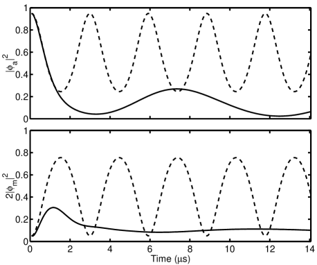
FIG. 2.: Time evolution of the atomic condensate $|\phi_{a}|^{2}$ and molecular condensate $2|\phi_{m}|^{2}$ for solely mean-field theory (dashed) and for the Hartree-Fock-Bogoliubov theory (solid).

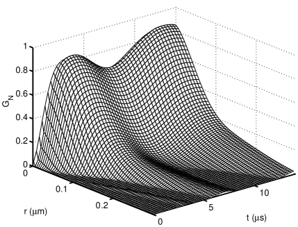
FIG. 3.: Evolution of the normal density.

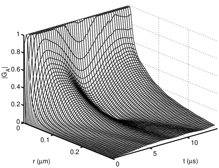
FIG. 4.: Evolution of the anomalous density.

In Fig. 4, we show the evolution of the anomalous fluctuations for this example. For a classical gas, the anomalous fluctuations are explicitly zero, so clearly the quantum statistics of the normal component generated here are not the usual classical thermodynamic equilibrium. One of the reasons for this is that there can never be an odd number of atoms in the thermal cloud since atoms are spontaneously generated from molecules in pairs. This situation is similar to the formation of a squeezed vacuum in optics using a laser pump to drive a parametric amplifier in order to produce photon pairs. Note the value of $|G_{A}(r)|$ near $r=0$ depends on $\sigma_{r}^{-1}$ and is not an observable.

In conclusion, the damping of the coherent atom-molecule oscillations is accompanied by an increase in density of the normal component. The behavior shown in Fig. 2 resolves the conceptual difficulty associated with the rapid atom-molecule oscillations predicted by mean-field theory—how can pairs of atoms find each other rapidly enough to form molecules at the predicted rate? The proper treatment of correlations shows that the oscillations are slower in frequency and moreover rapidly damped.

We would like to thank J. Cooper, E. Cornell, C. Wieman, and A. Andreev for helpful discussions. This work was supported by the Department of Energy.

REFERENCES

• [1] F. Dalfovo, S. Giorgini, L. P. Pitaevskii, and S. Stringari, Rev. Mod. Phys. 71, 463 (1999).
• [2] M. Edwards, P. A. Ruprecht, K. Burnett, R. J. Dodd, and C. W. Clark, Phys. Rev. Lett. 77, 1671 (1996).
• [3] J. E. Williams and M. J. Holland, Nature 401, 568 (1999); M. R. Matthews et al., Phys. Rev. Lett. 83, 2498 (1999).
• [4] D. F. Walls, Nature 324, 210 (1986).
• [5] E. Timmermans, P. Tommasini, R. Côté, M. Hussein, and A. Kerman, Phys. Rev. Lett. 83, 2691 (1999); E. Timmermans et al., Phys. Rep. 315 199 (1999);
• [6] F. A. Abeelen and B. J. Verhaar, Phys. Rev. Lett., 83 1550 (1999).
• [7] V. A. Yurovsky, A. Ben-Reuven, P. S. Julienne, and C. J. Williams, cond-mat/9903414.
• [8] P. D. Drummond, K. V. Kheruntsyan, H. He, Phys. Rev. Lett. 81, 3055 (1998).
• [9] S. Inouye et al., Nature 392, 151 (1998); J. Stenger et al., Phys. Rev. Lett. 82, 2422 (1999).
• [10] Ph. Courteille et al.. Phys. Rev. Lett. 81, 69 (1998); J. L. Roberts et al., ibid. 81, 5109 (1998).
• [11] P. S. Julienne et al., Phys. Rev. A 58, R797 (1998).
• [12] R. Wynar, R. S. Freeland, D. J. Han, C. Ryu, D. J. Heinzen et al., Science 287, 1016 (2000).