A scalar model of inhomogeneous elastic and granular media

Abstract

We investigate theoretically how the stress propagation characteristics of granular materials evolve as they are subjected to increasing pressures, comparing the results of a two-dimensional scalar lattice model to those of a molecular dynamics simulation of slightly polydisperse discs.

We characterize the statistical properties of the forces using the force histogram and a two-point spatial correlation function of the forces. For the lattice model, in the granular limit the force histogram has an exponential tail at large forces, while in the elastic regime the force histogram is much narrower and has a form that depends on the realization of disorder in the model. The behavior of the force histogram in the molecular dynamics simulations as the pressure is increased is very similar to that displayed by the lattice model. In contrast, the spatial correlations evolve qualitatively differently in the lattice model and in the molecular dynamics simulations. For the lattice model, in the granular limit there are no in-plane stress-stress correlations, whereas in the molecular dynamics simulation significant in-plane correlations persist to the lowest pressures studied.

I Introduction

Stress transmission in dry granular media is unusual because in these materials no simple relation exists between stress and strain[1, 2, 3, 4, 5]. Physical ingredients that give rise to this are that there are no tensile forces, that the particle deformations are very small, and that the particles can rearrange [6]. Over the last several years evidence has accumulated that force propagation in dry granular media could be fundamentally different than in elastic solids [3, 4, 7, 5, 8, 9]. Equations that have been proposed to describe stresses in lightly loaded granular media have the property that specification of boundary conditions at the top surface of the system is sufficient to determine the stresses throughout[4, 7, 5, 8, 9, 10, 11], in marked contrast to the elliptic equations of elasticity theory.

However, applying a large enough uniform pressure to a granular material will cause it to exhibit an elastic linear response to a small additional stress. This is because uniform pressure both inhibits rearrangements (because it suppresses Reynolds dilatancy) and compresses the contacts, so that the non-tensile constraint on the interparticle forces becomes irrelevant. Thus, if stress propagation in lightly loaded granular media is indeed substantially different than in elastic media, then subjecting the material to high pressures will change fundamentally the stress propagation characteristics.

This paper investigates theoretically the stress propagation in granular materials as they are subjected to increasing pressures. The goals of this work are to understand the physical mechanisms governing the evolution between granular and elastic behavior and to make specific experimental predictions for the behavior of granular media under increasing loads.

We study a two-dimensional model system and compare the results to molecular dynamics (MD) simulations of two-dimensional systems of slightly polydisperse discs. Numerical studies of statistical models of granular media, where geometrical complexity is modeled in terms of uncorrelated random variables, are much faster and simpler than molecular dynamics simulations. Models of this type hold promise as a means to obtaining insight into the physics underlying the force propagation in granular materials. Our model for the granular regime is the two-dimensional scalar $q$-model [10, 11]. Though the $q$-model has deficiencies [12], it is attractive because of its simplicity and its prediction of an exponential tail in the probability distribution of stress within a packing agrees with experiments [13, 14, 15] and with simulations [16, 17, 18, 19, 20, 21]. Our model for the elastic regime is a network of springs with a regular topology, with disorder introduced via randomly chosen spring constants[22, 23, 24, 25]. To model the crossover between the two regimes, we exploit our observation that the $q$-model can be written as a scalar elastic network subject to certain constraints. Enforcing these constraints to an increasing degree, which causes the force propagation behavior to evolve from that of an elastic system to that of the $q$-model, models the crossover between elastic and granular behavior by a particulate assemblage subjected to decreasing pressure.

We test the lattice model by comparing the results from the model to those of our MD simulations of two-dimensional systems of slightly polydisperse discs, focusing primarily on the probability distribution of stresses and on the two-point stress-stress correlation functions. The results of this investigation are mixed. The crossover in the force histogram between the elastic network and the $q$-model is strikingly similar to the crossover observed in the molecular dynamics simulations as the pressure on the system is decreased. However, the lattice model and the molecular dynamics simulation exhibit qualitatively different trends in the behavior of the two-point correlation functions of the stress.

The paper is organized as follows: Section II defines the scalar networks that we investigate. Section III details the process of generation, solution, and analysis of these networks and discusses the generation of the molecular dynamics simulations of slightly polydisperse discs. Section IV reports the results of the force distributions and spatial correlation functions for both the scalar lattice model and the MD simulations. Section V compares the results of the scalar lattice model, the MD simulations, and relevant experiments. Section VI summarizes and interprets our results. Appendix A calculates a finite-size correction to the in-plane stress-stress spatial correlation function for the $q$-model that is relevant to the interpretation of our numerical results.

II Scalar elastic networks and the $q$-model

This section discusses the relationship between the $q$-model and the elastic network studied in this paper. Both models are scalar and are defined on a two-dimensional lattice. A scalar model is appropriate for a spring network if either the the network is very highly stretched [22, 23, 26], or if the motions are constrained so that displacements are unidirectional [25]. We consider the second situation and denote the direction along which the motion occurs as $\hat{y}$, with positive $y$ pointing downwards.

Consider a network of nodes connected by springs on a diamond lattice as shown in Fig. 1, where the motion of every node is constrained to be along the vertical direction $\hat{y}$. Each spring has the same unstretched length, so that in the limit of zero load the system forms a regular lattice. The springs connecting the nodes have spring constants that are chosen independently from a fixed probability distribution. Periodic boundary conditions are imposed in the horizontal direction, and the locations of the nodes at the top and bottom boundaries are fixed so that the vertical displacement of all the nodes in these rows relative to the unloaded configuration are identical. We index the nodes so that a node in column $j$ in a row $i$ with odd (even) $i$ lies along the same vertical line as the other nodes in column $j$ in rows with odd (even) indices.

Let $y_{i,j}$ be the position of the node in row $i$ and column $j$ measured relative to its location in the absence of a load, and let $k_{i,j}^{l}$ and $k_{i,j}^{r}$ be the spring constants of the springs emanating downward from the node at row $i$ and column $j$. Every spring obeys Hooke’s law, so that $f_{i,j}^{l}$ and $f_{i,j}^{r}$, the forces exerted on node $(i,j)$ by the left and right springs below the node, are $k_{i,j}^{l}(y_{i,j}-y_{i+1,j-1})$ and $k_{i,j}^{r}(y_{i,j}-y_{i+1,j})$ for odd $i$ ($k_{i,j}^{l}(y_{i,j}-y_{i+1,j})$ and $k_{i,j}^{r}(y_{i,j}-y_{i+1,j+1})$ for even $i$). The system is then compressed by setting $y_{1,j}=(L_{y}-1)\Delta Y$ and $y_{L_{y},j}=0$ for all $j$, where rows $1$ and $L_{y}$ are the top and bottom rows, respectively, and $\Delta Y$ is the average strain. We define $F_{i,j}$ to be the total vertical force incident from above on node $(i,j)$, so that $F_{i,j}=f_{i-1,j-1}^{r}+f_{i-1,j}^{l}$. The forces and displacements are determined by balancing the forces at every node, $F_{i,j}=f_{i,j}^{l}+f_{i,j}^{r}$, and requiring that each $y_{i,j}$ be well-defined. This latter condition can be written as $\mathbf{S}=-[d]\mathbf{Y}$; here, $\mathbf{S}$ is the strain and $\mathbf{Y}$ is the displacement field [27].

In our spring networks, each spring constant has a value selected independently at random from various probability distributions that are described below. We obtain the forces and strains along each link of each network using the method outlined in Ref. [27].

This scalar elastic model is equivalent to a resistor network [22, 23, 25]. Forces and strains in the elastic system correspond to currents and voltages, respectively, in the resistor network. The requirement that the vertical forces at each node balance is equivalent to Kirchhoff’s current law, while the requirement that the position of each node is well-defined is equivalent to Kirchhoff’s voltage law.

A Comparison between the elastic model and the $q$-model.

The force $F_{i,j}$ incident from above on node $(i,j)$ is transmitted to the sites below in the two pieces $f_{i,j}^{l}$ and $f_{i,j}^{r}$. Because of force balance, one can always write

$$f_{i,j}^{l}=q_{i,j}F_{i,j},~{}~{}~{}f_{i,j}^{r}=(1-q_{i,j})F_{i,j}.$$ (1)

In a $q$-model, the $q_{i,j}$ are random variables that are chosen independently at every site. In an elastic network, Eq. (1) still holds, but the $q_{i,j}$ are determined by the configuration of random spring constants together with the requirement that the displacement field be single-valued. For spring constants that are chosen independently, the force along any branch will depend on the values of the spring constants throughout the system. Important consequences of this non-locality include the presence of spatial correlations between the $q_{i,j}$’s and a nontrivial relation between the distribution of spring constants and the distribution of the $q$’s, including possibly the presence of $q$’s that are negative, indicating the appearance of tensile forces in the network.

A key observation underlying our work is that the $q$-model is equivalent to an elastic network subject to the constraint that the strain on every spring in each row is identical. The strain need not be constant from one row to the next, but it is simplest to consider the case in which it is. Let the amount of strain be $\Delta Y$. Given the total force incident on node $(i,j)$ from above, $F_{i,j}$, if one chooses the spring constants to be

$$k_{i,j}^{l}=\frac{q_{i,j}F_{i,j}}{\Delta Y},~{}~{}~{}k_{i,j}^{r}=\frac{(1-q_{i,j})F_{i,j}}{\Delta Y},$$ (2)

then the force exerted down the left link emanating from node $(i,j)$ is $k_{i,j}^{l}\Delta Y=q_{i,j}F_{i,j}$, and the force exerted down the right link from node $i,j$ is $k_{i,j}^{r}\Delta Y=(1-q_{i,j})F_{i,j}$. This force redistribution rule is exactly that of of the $q$-model. Given the set of $q_{i,j}$ values and the forces at each node in the top row of the system, we can create an equivalent spring network in a layer-by-layer manner.

We do not implement explicitly a no-tensile force constraint in our networks, in contrast to the work of Refs. [24] and [25]. However, in the $q$-model limit, there are no tensile forces. Our molecular dynamics simulations of lightly loaded material yield force distributions much closer to that of the $q$-model than to those of the non-tensile elastic networks of Ref. [25].

To study the crossover between elastic and $q$-model behavior, we generate iteratively a sequence of networks that interpolate between the elastic and $q$-model limits. The procedure adjusts the spring constants to make the strain in the system more uniform while keeping the ratio of spring constants emanating from each node constant. At iteration $n$, the spring constants $k_{i,j}^{l}(n)$ and $k_{i,j}^{r}(n)$ are set to

$$k_{i,j}^{l}(n) = \frac{F_{i,j}(n-1)}{\Delta Y}q_{i,j}~{},$$ (4)

$$k_{i,j}^{r}(n) = \frac{F_{i,j}(n-1)}{\Delta Y}(1-q_{i,j})~{},$$ (5)

where $F_{i,j}(n-1)$ is the force through node $(i,j)$ at iteration $n-1$. The $q_{i,j}$ are kept fixed, and the iteration procedure is started with $F_{i,j}(0)=1$.

To characterize the crossover between elastic and $q$-model behavior as the iteration proceeds, we need to quantify the degree to which the constant-strain constraint is violated. We use as our measure of the spatial variation in the strain the dimensionless quantity

$$\delta{\mathcal{S}}_{N}\equiv\frac{\displaystyle\frac{1}{L_{x}(L_{y}-1)}\sum_{i=1}^{L_{y}-1}\sum_{j=1}^{L_{x}}\frac{1}{2}\left((\delta Y_{i,j}^{l}-\overline{\delta{Y}})^{2}+(\delta Y_{i,j}^{r}-\overline{\delta{Y}})^{2}\right)}{\overline{\delta Y}^{2}}$$ (6)

where $\delta Y_{i,j}^{l}=Y_{i,j}-Y_{i+1,j-1}$ and $\delta Y_{i,j}^{r}=Y_{i,j}-Y_{i+1,j}$ for odd $i$ ($\delta Y_{i,j}^{l}=Y_{i,j}-Y_{i+1,j}$ and $\delta Y_{i,j}^{r}=Y_{i,j}-Y_{i+1,j+1}$ for even $i$), and

$$\overline{\delta{Y}}=\frac{1}{L_{x}(L_{y}-1)}\sum_{i=1}^{L_{y}-1}\sum_{j=1}^{L_{x}}\frac{1}{2}(\delta Y_{i,j}^{l}+\delta Y_{i,j}^{r})=\Delta Y.$$ (7)

Here, $L_{y}$ and $L_{x}$ are the number of rows and columns, respectively. In the elastic limit $\delta{\mathcal{S}}_{N}\approx 0.2$, and as discussed above, $\delta{\mathcal{S}}_{N}$ is zero for the $q$-model.

III Methods

A Scalar lattice model

We consider diamond-shaped lattices with springs on each link, as shown in Fig. 1. The positions of the top and bottom node layers are fixed and periodic boundary conditions are imposed in the transverse direction. The forces along all the links depend on the choice of spring constants, $\{k_{i,j}\}$, and are calculated using the node-potential method described in Ref. [27]. The overall strain for each network is scaled so that the average vertical force through each node is normalized to unity,

$$\bar{F}\equiv\frac{1}{L_{x}L_{y}}\sum_{i=1}^{L_{y}}\sum_{j=1}^{L_{x}}F_{i,j}=1,$$ (8)

where the sum is over the nodes in the network.

Networks of height $L_{y}=500$ are used, with analysis performed on separate groups of layers to distinguish between edge and bulk effects. The widths $L_{x}=16$ and $128$ are powers of 2 in order to take advantage of FFT techniques in the calculation of spatial correlation function values described below. The number of realizations averaged over varies from 10 to 50, depending on lattice size and number of iterations.

For the elastic regime, we use four different distributions of spring constants: uniform distribution of $k^{-1}$ for $k^{-1}\in(0,1)$, gaussian distribution of $k^{-1}$ with the configuration average $(\overline{k^{-1}})=1$ and standard deviation $\sigma_{k^{-1}}=0.5$, uniform distribution of $k$ with $k\in(0,1)$, and gaussian distribution of $k$ with $\bar{k}=1$ and $\sigma_{k}=0.5$. We construct networks with $L_{x}=16$ and $128$ with 50 and 25 realizations, respectively.

For the $q$-model regime, a uniform distribution of $q$ with $q\in(0,1)$ is used. We implement the iterative scheme with networks of size $L_{x}=16$ and $128$ with 50 and 10 realizations, respectively, for 100 iterations.

The local stress redistribution in a real granular material depends on microscopic details such as particle shape, friction characteristics, and preparation history. Instead of attempting to model the local force redistribution rules microscopically, our statistical models treat them as random variables chosen from different probability distributions. Since these probability distributions are not known a priori, we wish to identify and study properties that are not sensitive to the choice of the probability distribution governing the local force redistribution in the model. We focus on $P(F)$, the probability distribution of stresses at the nodes; $\tilde{P}(q)$, the probability distribution of the redistribution fractions $q$; and the spatial correlation functions of the force fluctuations about the mean values [28],

$$C_{k}(j)=\frac{1}{L_{y}-k}\sum_{l=1}^{L_{y}-k}\left(\frac{\displaystyle\sum_{m=1}^{L_{x}}\delta F_{l,m}\delta F_{l+k,m+j}}{\displaystyle\sum_{m=1}^{L_{x}}\delta F_{l,m}^{2}}\right),~{}~{}~{}\tilde{C}_{k}(j)=\frac{1}{L_{y}-k}\sum_{l=1}^{L_{y}-k}\left(\frac{\displaystyle\sum_{m=1}^{L_{x}}\delta q_{l,m}\delta q_{l+k,m+j}}{\displaystyle\sum_{m=1}^{L_{x}}\delta q_{l,m}^{2}}\right),$$ (9)

where $\delta F_{i,j}=F_{i,j}-\bar{F}$ and $\delta q_{i,j}=q_{i,j}-\bar{q}$; $\bar{F}$ is the average force and $\bar{q}$ is the average $q$ value. The indices $l$ and $m$ in Eq. 9 label layers and columns, respectively, while $k$ and $j$ are the spatial separation in layers and columns. These correlation functions are normalized so that $C_{0}(0)=1$ and $\tilde{C}_{0}(0)=1$. Positive values (correlation) indicate a tendency for nodes separated by $k$ rows vertically and $j$ columns horizontally to be either both above or both below the mean, while negative values (anti-correlation) indicates opposite behavior of one above and one below the mean.

B Molecular dynamics simulations

Here we discuss our molecular-dynamics (MD) simulations to used to generate 2-D packings of discs. Varying the ratio of external load pressure to particle stiffness induces crossover between granular and elastic behavior. We calculate the probability distributions and corresponding spatial correlation function values for forces and redistribution fractions $q$ that are analogous to those in the scalar model.

Our simulations employ a method similar to that used by Durian and collaborators for sheared foams [29, 30, 31], in addition incorporating kinetic friction, contact damping, and particle rotation, and using two different repulsive interparticle force laws (linear and Hertzian).

1 MD interaction rules

The discs in our simulation are all of identical mass $m_{D}=1$ and interact via purely repulsive normal contact forces and kinetic friction. The interaction force between two discs whose centers are at positions $\vec{r}$ and $\vec{r}_{j}$ with radii $a_{i}$ and $a_{j}$ is non-zero only if their separation $\delta r_{i,j}\leq 0$, where

$$\delta r_{i,j}=\left|\vec{r}_{i}-\vec{r}_{j}\right|-(a_{i}+a_{j}).$$ (10)

The normal contact force ${\mathcal{F}}_{i,j}$ is calculated from the overlap $|\delta r_{i,j}|$. We examine two force laws. The first is a linear force law based on a spring-like restoring force that yields

$${\mathcal{F}}_{i,j}=K_{i,j}\left|\delta r_{i,j}\right|,$$ (11)

with $K_{i,j}=(1/K_{i}+1/K_{j})^{-1}$, where $K_{d}$ is the spring constant for disc $d$. The second is a non-linear force law based on Hertzian contacts between spheres[32],

$${\mathcal{F}}^{[\mathrm{HC}]}_{i,j}=D^{-1}(\frac{1}{a_{i}}+\frac{1}{a_{j}})^{-\frac{1}{2}}\left|\delta r_{ij}\right|^{\frac{3}{2}},$$ (12)

where $D=\frac{3}{2}\left((1-\sigma^{2})/E\right)$, with $\sigma$ and $E$ being the material properties Poisson’s ratio and Young’s modulus, respectively. For both force laws, the forces are directed so as to separate the overlapping discs. To calculate forces generated by interactions with walls, we assume the walls to be discs of infinite radius.

Kinetic friction is incorporated into the disc interactions although static friction is not. The introduction of frictional forces causes the discs to rotate; however, the frictional force is zero at mechanical equilibrium. The kinetic friction force $f_{i,j}$ for contact between discs $i$ and $j$ is

$$f_{i,j}=\mu{\mathcal{F}}_{i,j},$$ (13)

where $\mu$ is the coefficient of kinetic friction, and is directed opposite to the contact point velocity $\vec{v}^{\mathrm{cp}}_{i,j}$. For disc $i$, this velocity $\vec{v}^{\mathrm{cp}}_{i,j}$ is related to disc velocities $\vec{v}_{i}$ and $\vec{v}_{j}$, the angular velocities $\omega_{i}$ and $\omega_{j}$, and directional vector $\hat{r}=(\vec{r}_{i}-\vec{r}_{j})/|\vec{r}_{i}-\vec{r}_{j}|$ by

$$\vec{v}^{\mathrm{cp}}_{i,j}=\vec{v}_{i,j}-\left(\vec{v}_{i,j}\cdot\hat{r}\right)\hat{r}+\left(a_{i}\vec{\omega}_{i}+a_{j}\vec{\omega}_{j}\right)\times\hat{r},$$ (14)

where $\vec{v}_{i,j}=\vec{v}_{i}-\vec{v}_{j}$.

Damping during contact between discs $i$ and $j$ is used as an additional means of dissipating kinetic energy. It is generated by applying to disc $i$ a force ${\mathcal{F}}_{\mathrm{D}}$ and torque $\Gamma_{\mathrm{D}}$ given by

$${\mathcal{F}}_{\mathrm{D}} = -\lambda_{\mathrm{trans}}v^{\prime}_{i},$$ (16)

$$\Gamma_{\mathrm{D}} = -\lambda_{\mathrm{ang}}\omega^{\prime}_{i},$$ (17)

where $v_{i}^{\prime}$ is the translational velocity of disc $i$ relative to the interaction center of mass for the two discs $i$ and $j$ that are in contact and $\omega^{\prime}_{i}$ is its angular velocity relative to the total angular momentum of the disc pair. $\lambda_{\mathrm{trans}}$ and $\lambda_{\mathrm{ang}}$ are damping constants. This process conserves both translational and angular momentum. Energy is directly removed from the system as opposed to being converted between translational and rotational motion.

The bottom and top walls have mass $m_{W}$ and are constrained to move only vertically. An inward force of magnitude $F_{\mathrm{wall}}$ is applied to each wall in order to compress the system. Damping of the wall motion suppresses volume oscillations and serves as the primary means of energy dissipation. The damping force ${\mathcal{F}}_{\mathrm{WD}}$ on a wall is

$${\mathcal{F}}_{\mathrm{WD}}=-\lambda_{W}v_{W},$$ (18)

where $v_{W}$ is the velocity of the wall and $\lambda_{W}$ is the wall damping constant.

2 MD implementation

Ensembles of systems of $N=1024$ discs of average radius $a_{D}$ are generated by starting with triangular array of $\sqrt{N}$ rows and $\sqrt{N}$ discs per row placed in a horizontally periodic system with both height and width $L=2.273a_{D}\sqrt{N}$. For the data shown here, discs are placed in the system at positions $(L(n_{x}+0.05)/\sqrt{N},L(n_{y}+0.5)/\sqrt{N})$ for odd $n_{y}$ and $(L(n_{x}+0.55)/\sqrt{N},L(n_{y}+0.5)/\sqrt{N})$ for even $n_{y}$, with indices $n_{x}$ and $n_{y}$ running from 0 to $\sqrt{N}-1$. In practice, discs with gaussian distributed polydispersity of $\sigma_{a}=0.1a_{D}$ placed on this triangular array do not overlap. The results obtained are not sensitive to initial disc placement. The system is then compressed by the application of an inward force on the top and bottom walls. All discs have the same spring constant $K_{d}\equiv K=1$. The coefficient describing wall damping is set to $\lambda_{W}/m_{W}=1$. Damping coefficients for translational and angular motion for disc contacts are set to $\lambda_{\mathrm{trans}}/m_{D}=1$ and $\lambda_{\mathrm{ang}}/I_{D}=4.1$, where $I_{D}=\frac{1}{2}m_{D}a_{D}^{2}$ is the moment of inertia for a disc with radius $a_{D}$. The coefficient of kinetic friction is set to $\mu=0.2$ for both disc-disc and disc-wall contacts. Comparisons with samples produced without disc-contact damping or kinetic friction revealed no measurable differences in force probability distributions or in the two-point force correlation function. Incorporating additional energy-dissipation mechanisms allows systems to reach mechanical equilibrium more rapidly. The end time for each compression stage is chosen so that the average residual kinetic energy for each disc is equivalent to translational movement of approximately or less than $0.01a_{D}$ in unit time. Because of the increased external energy input, systems at higher compressions are allowed a less restrictive limit of approximately $0.05a_{D}$. Visual inspection of final configurations do not reveal significant fluctuations in time in contact network topology or force magnitude in load-bearing structures. Comparisons with test systems with longer run times also do not show any significant quantitative differences.

For a system of fixed size $L$, the typical compression of the system can be controlled through variations in the disc spring constant $K$ or applied external force $F_{\mathrm{wall}}$. Typical relative particle deformations $\delta{\mathcal{R}}$ is given by

$$\delta{\mathcal{R}}\equiv\frac{1}{N_{C}}\sum_{(i,j)}\frac{|\delta r_{i,j}|}{(a_{i}+a_{j})}=\frac{1}{N_{C}}\sum_{(i,j)}\frac{{\mathcal{F}}_{i,j}}{K_{i,j}}(a_{i}+a_{j})^{-1}\approx\frac{F_{\mathrm{wall}}\left(\frac{L}{a_{D}}\right)^{-1}}{\frac{K}{2}}(2a_{D})^{-1}=\frac{F_{\mathrm{wall}}}{LK}=\frac{\Pi}{K},$$ (19)

where $N_{C}$ is the total number of contacts, the sums are over pairs of discs $i$ and $j$ in contact, and $\Pi\equiv F_{\mathrm{wall}}/L$ is the external pressure. This estimate is approximate due to geometric factors and distributional fluctuations; however, the scaling of deformations to $\Pi/K$ should hold generally. In our simulations, the disc spring constant $K$ is held fixed and the pressure $\Pi$ is varied to induce crossover between granular and elastic behavior. We define the reference pressure $\Pi=\Pi_{0}$ such that the relative particle deformation $\delta{\mathcal{R}}\approx 6.25\times 10^{-4}$. The reference compression pressure $\Pi_{0}$ yields a force histogram typical of the granular range, as discussed below in Sec. IV. After the initial compression with $\Pi=\Pi_{0}$, the applied pressure is increased in stages to $\Pi=100\Pi_{0}$, at which $\delta{\mathcal{R}}\approx 0.01$. We also decrease the pressure from the initial $\Pi=\Pi_{0}$ configuration down to $\Pi=0.01\Pi_{0}$ ($\delta{\mathcal{R}}\approx 10^{-6}$) in order to approach the zero-deformation limit. Fig. 2 shows a sample MD system subjected to the pressures $0.1\Pi_{0}$, $\Pi_{0}$, $10\Pi_{0}$, and $50\Pi_{0}$.

For spheres with Hertzian contacts (using Eq. 12), the deformation can be approximated by $\delta{\mathcal{R}}^{\mathrm{[HC]}}\approx\left(\frac{\Pi D}{2a_{D}}\right)^{\frac{2}{3}}$. For our simulations $D$ is chosen to yield deformations of the same order of magnitude as the linear contacts at the compression $\Pi=\Pi_{0}$. The pressures studied are the same as for the linear spring contact systems.

IV Results

A Scalar lattice model

Here we present our results for the scalar lattice models. We study how the probability distribution of total vertical force $F$ incident on a node from above $P(F)$ and the two-point force correlation function $C_{k}(j)$ characterize the behavior in scalar elastic lattice networks in which the constant-strain constraint is enforced to varying degrees. In the $q$-model both $P(F)$ and in-plane force-force correlation function $C_{0}(j)$ exhibit robust behavior for generic choices of probability distributions of $q$’s. We investigate the degree to which these quantities depend on the choice of spring constant distributions in the elastic networks, and discuss the crossover of $P(F)$ and $C_{0}(j)$ between the elastic and $q$-model behavior as the constant-strain constraint is implemented with increasing accuracy.

1 Results for the $q$-model

In the $q$-model, the force histogram $P(F)$ decays exponentially at large forces[11] and $C_{0}(j)$ is zero for non-zero $j$ [11, 33, 34]. These properties hold for a wide variety of choices of the distribution of $q$-values.

Our results for the crossover from elastic to $q$-model behavior are obtained for the specific choice that the $q$’s are uniformly distributed in $[0,1]$. A two-dimensional $q$-model with this distribution of $q$’s yields[11]

$$P(F)=4Fe^{-2F}.$$ (20)

For a system of infinite lateral extent, the in-plane force-force correlation function $C_{0}(j)=\delta_{j0}$ where $\delta_{j0}$ is the Kronecker delta function [11]. For a system of finite width $L_{x}$, force correlations must arise because all forces are positive and the total force through a layer is fixed. As discussed in Appendix A, assuming that this mechanism is the only one giving rise to correlations, one obtains that a 2-D system of lateral extent $L_{x}$ has $C_{0}(j)$ given by

$$C_{0}(j\neq 0)=-(L_{x}-1)^{-1}.$$ (21)

This form for $C_{0}(j)$ agrees with our numerical results for the $q$-model on lattices of finite width.

2 Elastic networks

For elastic networks with different distributions of spring constants, the probability distribution of vertical force $P(F)$, shown in Figs. 3, is narrower than that of the $q$-model. Its functional form depends on the choice of spring constant distribution. Choosing the spring constants $k$ from a distribution either uniform in $k$ or gaussian in $k$ yields $P(F)$’s that are roughly gaussian while the $P(F)$’s for networks for distributions uniformly distributed or gaussian in $k^{-1}$ display a tail at large $F$ that is consistent with an exponential decay. Networks with gaussian distributed $k$ or $k^{-1}$ exhibit narrower $P(F)$’s than their counterparts with uniformly distributed $k$ or $k^{-1}$.

In contrast to the behavior of the force probability distribution $P(F)$, the force-force correlation function values $C_{k}(j)$ are quantitatively indistinguishable for all the distributions of spring constants that we examined, as shown in Fig. 4. For $C_{0}(j)$, the force-force correlation function within the same layer, we see a strong anti-correlation for $j=1$ of magnitude $\sim 0.30$ that decays within $j\leq 8$. For vertical separation $k>0$, we see a simultaneous reduction in peak magnitude (at $j=0$) and broadening of peak width but with the anti-correlation signature and decay joining the curve laid out by $k=0$.

The probability distributions of redistribution fraction $q$, $\tilde{P}(q)$, shown in Fig. 5, are roughly gaussian and peaked at $q=\bar{q}\equiv 0.5$ for all distributions of spring constants examined. The widths of the $\tilde{P}(q)$ depend on the choice of distribution of spring constants, with the gaussian distributed $k$ and $k^{-1}$ once again being narrower (standard deviation $\sigma_{q}\approx 0.16$ and $0.15$, respectively) than their uniformly distributed counterparts ($\sigma_{q}\approx 0.25$ for random $k$ and $\sigma_{q}\approx 0.21$ for random $k^{-1}$). All of the elastic networks display significant correlations between $q$’s at different nodes as demonstrated in Fig. 6, which shows the correlation function $\tilde{C}_{k}(j)$ for all the random distributions. The correlations between $q$’s are an important factor in determining the statistical distribution of the forces in these systems; Fig. 7 shows that a $q$-model system with the same $\tilde{P}(q)$ as an elastic network with a uniform distribution of $k$ but with no correlations between the $q$’s yields a $P(F)$ markedly different from the elastic network.

No differences between the bulk (layers 201-300) and edge (layers 1-100 and 401-500) sections are detected in the distributions $P(F)$ and $\tilde{P}(q)$ or the correlation functions $C_{k}(j)$ and $\tilde{C}_{k}(j)$. The results for lattices with $L_{x}=128$ are the same within statistical errors to the results from $L_{x}=16$ lattices.

In the elastic networks, forces in less than 1% of the branches are tensile, and no node in any of the networks is subject to a tensile net force. Our results for $P(F)$ for uniformly distributed $k$’s are very similar to those reported in Sexton et al. [25], where a non-tensile force constraint is enforced.

3 Iterated networks– the $q$-model limit

We now discuss the networks generated by our iterative algorithm for converting an elastic network to a $q$-model system. First, we verify that the generated networks do eventually converge to the $q$-model. After 100 iterations, the forces along the links of the iterated spring network are identical to those of the corresponding $q$-model to within $10^{-4}$.

A subtle point in the method is that our iterative scheme yields a configuration in which the forces at the top and bottom boundaries of the iterated network may have nonzero spatial correlations, as the initial iteration $n=0$ system is elastic. As one proceeds away from the top and bottom boundaries, these correlations decay via a diffusive process that takes on the order of $L_{x}^{2}$ layers [11]. Thus, forces at different sites in the same layer are effectively uncorrelated only for systems with large aspect ratios. This result is consistent with our numerical observation that in fully iterated systems, correlations between forces at different sites in the same layer are present throughout the $L_{x}=128$ systems, while they are only present in the top- and bottom-most 200 layers of $L_{x}=16$ systems.

4 Iterated networks– crossover between elastic and $q$-model behavior

In the iterated networks the target values of the $q_{i,j}$ are fixed at the outset of iteration procedure. The initial state (zeroth iteration) is an elastic network with spring constants given by $k_{i,j}^{l}=q_{i,j}/\Delta Y$ and $k_{i,j}^{r}=(1-q_{i,j})/\Delta Y$. Therefore, the initial probability of node forces $P(F)$ and the spatial correlation function $C_{0}(j)$ are those of elastic networks with spring constants chosen from a uniform distribution of $k$. The realized $q$ distribution $\tilde{P}(q)$ (as opposed to the distribution of the target $q$ values) is peaked at $q=0.5$ and its spatial correlation function $\tilde{C}_{k}(j)$ reveals slight nearest-neighbor correlations for $k=0$ and anti-correlations at $j=0$ for $k>0$, once again matching elastic-regime behavior.

The probability distribution of node forces, $P(F)$, is shown in Fig. 8(a) for different values of iteration number $n$. As the number of iterations is increased, the $P(F)$ develops an exponential tail at large forces. Fig. 8(b) shows the probability distribution of the $q$’s, $\tilde{P}(q)$, versus the number of iterations. $\tilde{P}(q)$ approaches the target form of a uniform distribution after roughly 10 iterations.

Fig. 9(a) shows our results for nearest-neighbor in-plane and vertical force-force correlation function values $C_{0}(1)$ and $C_{2}(0)$ as the number of iterations $n$ is increased. Fig. 9(b) shows the corresponding force-fraction $q$-$q$ correlations $\tilde{C}_{0}(1)$ and $\tilde{C}_{2}(0)$. While only about 10 iterations are necessary before the nearest-neighbor spatial correlations between $q$ values go to zero, in-plane force-force correlations are still present after 100 iterations although much reduced in magnitude from the initial elastic (iteration $n=0$) value and approaching asymptotically the expected zero-correlation value.

The quantity $\delta{\mathcal{S}}_{N}$ that we use to characterize the crossover between elastic and $q$-model behavior is defined in Sec. II. As Fig. 10 demonstrates, we observe $\delta{\mathcal{S}}_{N}$ decreasing as the number of iterations $n$ is increased according to a power law. A fit that assumes the dependence is of the form $\delta{\mathcal{S}}_{N}\propto n^{\alpha}$ yields $\alpha=-1.68\pm 0.02$.

B Results of molecular dynamics simulations

Here we discuss the results of our MD simulations. Fig.11 shows $P(F)$, the probability distribution of vertical forces $F=\vec{{\mathcal{F}}}\cdot\hat{y}$, for MD systems under various applied pressures $\Pi$. As with the scalar model, $F$ has been normalized so that the average vertical force $\bar{F}=1$ for each system configuration. The progression of $P(F)$ as pressure is increased is very similar both qualitatively and quantitatively to the crossover from granular to elastic behavior in the scalar model lattice systems. We calculate the force-force correlation values $C_{0}(j)$, shown in Fig. 11(b), by defining discs to be in plane with a tolerance of $\pm 0.10a_{D}$ and $j$ in units of average disc diameter $2a_{D}$. In contrast with the scalar model behavior, the MD systems exhibit a significant nearest-neighbor anti-correlation for all applied external pressures. These results for $P(F)$ and $C_{0}(j)$ are independent of whether the samples are compressed in stages or directly at a fixed pressure $\Pi$.

We define the $q$ value of a disc as the fraction of total vertical force received from its topward neighbors that is transferred to its bottom leftward neighbors. The probability distribution of $q$ values, $\tilde{P}(q)$ is shown in Fig.12. We also calculate the $q$-$q$ correlation values $\tilde{C}_{0}(j)$ and $\tilde{C}_{k}(0)$, although the large errors prevent the extraction of quantitative trends. Narrowing the statistical errors would be computationally prohibitive.

The number of contacts increases significantly with the pressure, as shown in Fig. 13. As the magnitude of the typical overlap increases, additional contacts are formed. The number of contacts at low pressures is below the theoretically predicted average of $Z=2d$[9], where $d$ is the dimension of the system, because the polydispersity in radii and the lack of gravity allow for the existence of “rattlers” which do not support any of the external load.

Our results for the Hertzian contact systems are indistinguishable from those of the linear springs throughout most of the range of pressures explored. At higher pressures $\Pi$ ($\Pi\geq 35\Pi_{0}$), the added stiffness of the Hertzian contacts leads to the slower narrowing of $P(F)$.

V Comparison of results of MD simulations and of scalar elastic networks

Here we compare the behavior observed in the MD simulations and in the scalar elastic networks. Because different schemes are used to induce the granular-elastic crossover in the two systems (iterations in the scalar networks and external pressure for MD), we need to establish a common measure to quantify a system’s position within the crossover region. As the evolution of the probability distribution of vertical forces, $P(F)$, is qualitatively and quantitatively similar in the network model and in the MD simulations, we use matches in its form to establish a relationship between iteration number $n$ and applied pressure $\Pi$. Fig. 14(a) shows matches in form between linear-force-law MD packings and iterated scalar network systems for $\Pi/\Pi_{0}=100$ and iteration $n=0$, $\Pi/\Pi_{0}=10$ and $n=10$, and $\Pi/\Pi_{0}=1$ and $n=100$ systems. From these matchings, we map the iteration number $n$ in the scalar networks to the equivalent applied pressure $\Pi_{\mathrm{eq}}(n)$ in the MD using the simple scaling [35]:

$$\frac{\Pi_{\mathrm{eq}}(n)}{\Pi_{0}}=\frac{100}{n}.$$ (22)

We perform a check on this proposed scaling by considering the analogous quantities of deviation from constant strain in scalar systems $\delta{\mathcal{S}}_{N}$, given by Eq. 6, and deviation from the infinitely hard, zero-deformation limit in MD systems calculated by

$$\delta{\mathcal{S}}_{MD}\equiv\frac{1}{N_{C}}\sum_{(i,j)}\frac{|\delta r_{i,j}|^{2}}{(a_{i}+a_{j})^{2}}$$ (23)

where $N_{C}$ is the total number of contacts and the sum is over pairs of discs $i$ and $j$ in contact. We match $\delta{\mathcal{S}}$ values for $\Pi/\Pi_{0}=10$ and $n=10$ by scaling the square deviation for the scalar network systems by a constant factor of 0.030. Fig. 14(b) shows that this scaling yields reasonable agreement between $\delta{\mathcal{S}}_{N}$ and $\delta{\mathcal{S}}_{MD}$ over the crossover region.

In contrast to the agreement in the trends of $P(F)$, qualitative differences exist between the scalar network model and the MD simulations in spatial correlation function values $C_{j}(k)$. Fig. 15(a) shows the nearest-neighbor in-plane and vertical force-force correlation values, $C_{0}(1)$ and $C_{2}(0)$, for the crossover between elastic and granular regimes. While the MD systems exhibit a significant in-plane nearest-neighbor anti-correlation throughout the crossover, a decrease in its magnitude is seen in the scalar networks as the systems change from elastic to granular. MD systems do not exhibit strong vertical correlations, in contrast with the scalar networks whose $C_{2}(0)$ value increases significantly as the granular limit is approached.

The large statistical uncertainties in our $q$-$q$ correlation functions for MD systems restrict us to making only qualitative behavior descriptions. The trend for in-plane nearest-neighbor correlation behavior $\tilde{C}_{0}(1)$ in both systems is similar. However, qualitative differences exist for vertical correlation value $\tilde{C}_{2}(0)$: the MD systems display consistent anti-correlation behavior, while the scalar networks display anti-correlation behavior in the elastic regime which decays rapidly to uncorrelated behavior as the granular limit is approached.

Our work indicates that experiments on granular media at high pressures should yield a force histogram that differs qualitatively from that observed at lower pressures. Experiments by Howell et al. [36] as well as experiments and simulations by Makse et al. [37] are in qualitative agreement with this result. Howell et al. [36] control the transition between granular and elastic behavior of slowly sheared systems in a 2-D Couette geometry by varying the packing fraction $\gamma$ within a range $0.77\leq\gamma\leq 0.81$. The average force/length on a particle increases with $\gamma$. For lower values of $\gamma$, the distribution of large stresses is asymptotically exponential, while the distribution of stresses has a gaussian form at higher packing fractions $\gamma$. Makse et al. [37] apply increasing pressure to three-dimensional packings of spherical glass beads to achieve the crossover between granular and elastic behavior and also perform MD simulations on 3-D systems. Makse et al. observe a crossover in the force histogram $P(F)$ in a pressure range that is consistent with our 2-D MD results.

An interesting question is whether the persistent in-plane nearest-neighbor anti-correlation in the forces that is observed in the MD simulations is present in experimental systems. Mueth et al. [15] do not find evidence of correlations between different sites in the same horizontal layer; any nearest-neighbor anti-correlation in the experiment is smaller than the experimental resolution. However, they measure a different correlation function, $K_{1}(r)$, defined as

$$K_{1}(r)=\frac{\displaystyle\sum_{i=1}^{N_{B}}\sum_{j=i+1}^{N_{B}}\delta(r_{ij}-r)f_{i}f_{j}}{\displaystyle\sum_{i=1}^{N_{B}}\sum_{j=i+1}^{N_{B}}\delta(r_{ij}-r)},$$ (24)

where the sums are over the $N_{B}$ particles in the bottom layer, $f_{i}$ is the force at position $r_{i}$ in the bottom layer and $r_{ij}=|\vec{r}_{i}-\vec{r}_{j}|$. Calculation of $K_{1}(r)$ from the numerical data for our MD simulations yields values of the correlation function that are smaller than the error bars in the experiment. Comparison with Ref. [15] is necessarily qualitative since the experiments measure the properties at the surface of a 3-D packing while our MD results are calculated using numerical data from the bulk of a 2-D system.

VI Discussion

We have investigated the crossover between elastic and granular stress transmission in both a 2-D scalar lattice model and in molecular dynamics simulations of slightly polydisperse discs. The evolution of $P(F)$, the probability distribution of stresses, is very similar in the lattice model and in the MD. However, the behavior of the spatial correlation functions for stress, $C_{k}(j)$, differs qualitatively.

Our investigations of the scalar model have several implications for the development of granular media models. First, we have shown that implementing a local constraint can convert an elastic network to a $q$-model. This constraint has the natural physical interpretation that the strain in the system must be uniform; it is plausible that rearrangements would prevent strain gradients from forming. Second, implementing this constraint to increasing accuracy causes the force histogram $P(F)$ to evolve in a manner similar to that observed in the MD simulation as the pressure is decreased. $P(F)$ has a tail consistent with exponential decay at large forces in the granular limit, while the $P(F)$ for the highly compressed system is much narrower and decays more quickly at large forces. We note that implementing a non-tensile force constraint alone, as in Ref. [25], yields gaussian decay in $P(F)$ at large forces even at the lowest pressures, in qualitative disagreement with the MD results of us and others [16, 18, 37].

While this success in describing the evolution of the force histogram and the scalar model’s simplicity in both formulation and implementation make it an attractive platform for the study of media models, the discrepancy in the behavior of the correlation function behavior with the MD simulation results needs to be addressed. The scalar model assumes explicitly that in the granular regime the stress redistribution fractions $q$ at different sites are uncorrelated. The extent to which this condition is valid needs to be examined in more detail. Spatial correlations of the $q$’s can strongly affect the probability distribution of stress $P(F)$ [38, 28] but the degree to which these correlations exist in real packings has not been settled. A possible source of spatial correlations in the $q$’s is the constraint that non-tensile vector forces must be balanced. However, vector generalization of $q$-model systems that have been proposed to date have required arbitrary constraints to be imposed to limit the scale of stress components perpendicular to the direction of applied force [12]. Clarification of the roles of vector force balance and contact formation is key to identifying and characterizing the processes governing stress transmission beyond those that have been implemented in the scalar model.

In conclusion, we have shown that similarities exist in the evolution of the probability distribution of stresses $P(F)$ in the crossover between elastic and granular regimes for a scalar lattice model and MD simulations of slightly polydisperse discs. However, the systems exhibit qualitative differences in the two-point force correlation function $C_{k}(j)$. Further investigation of the systematic influences leading to the spatial correlations between forces is necessary for the development of a successful model of stress transmission in granular media.

A Finite-size correction to correlation function calculation

In the $q$-model in the limit of infinite size, forces at different sites in the same layer are completely uncorrelated. In a system of finite transverse extent, the requirements that the total force through every layer is identical and there are no tensile forces lead to a finite-size correction to the correlation function. This appendix discusses this correction.

We characterize the correlations between force fluctuations on sites in the same row using the correlation function

$$C_{0}(j)=\frac{1}{L_{y}}\sum_{l=1}^{L_{y}}\left(\frac{\displaystyle\sum_{m=1}^{L_{x}}\delta F_{l,m}\delta F_{l,m+j}}{\displaystyle\sum_{m=1}^{L_{x}}\delta F_{l,m}^{2}}\right),$$ (A1)

where $\delta F_{l,m}=F_{l,m}-\bar{F}$ is the deviation of the force at a site in row $l$ and column $m$ from the average force $\bar{F}$. For the $q$-model with a uniform distribution of $q$’s, in a system of infinite transverse extent this correlation function is [11]

$$C_{0}(j)=\left\{\begin{array}[]{ll}1&j=0\\ 0&j\neq 0\end{array}\right..$$ (A2)

This result follows from the fact that $P(F_{\alpha},F_{\beta})$, the probability that the force through node $\alpha$ is $F_{\alpha}$ and the force through node $\beta$ at the same horizontal level is $F_{\beta}$, is factorizable:

$\displaystyle P(F_{\alpha},F_{\beta})=P(F_{\alpha})P(F_{\beta}),$

As a result, for $\alpha\neq\beta$

$$\langle\delta F_{\alpha}\delta F_{\beta}\rangle = \lim_{L_{x},L_{y}\rightarrow\infty}\frac{1}{L_{y}L_{x}}\sum_{l=1}^{L_{y}}\sum_{m=1}^{L_{x}}\delta F_{l,m}\delta F_{l,m+j}$$ (A3)

$$= \int_{0}^{\infty}\int_{0}^{\infty}dF_{\alpha}dF_{\beta}\ \delta F_{\alpha}\ \delta F_{\beta}\ P(F_{\alpha},F_{\beta})$$ (A4)

$$= \int_{0}^{\infty}\int_{0}^{\infty}dF_{\alpha}dF_{\beta}\ \delta F_{\alpha}\ \delta F_{\beta}\ P(F_{\alpha})P(F_{\beta})$$ (A5)

$$= \left(\int_{0}^{\infty}dF_{\alpha}\ \delta F_{\alpha}\ P(F_{\alpha})\right)\left(\int_{0}^{\infty}dF_{\beta}\ \delta F_{\beta}\ P(F_{\beta})\right)$$ (A6)

$$= \left[\int_{0}^{\infty}dF\delta F\ P(F)\right]^{2}$$ (A7)

$$= \left[\int_{0}^{\infty}dF(F-\bar{F})\ P(F)\right]^{2}$$ (A8)

$$= \left[\bar{F}-\bar{F}\right]^{2}$$ (A9)

$$= 0.$$ (A10)

On a lattice of finite width ($L_{x}$ sites), the multipoint force probability distribution function must be consistent with the facts that first, the total force down every layer is fixed, and second, no force is negative. This implies that

• The maximum force on any node in any layer cannot be larger than $F_{\mathrm{max}}=L_{x}\bar{F}$, and

• The force $F_{\alpha}$ at a node $\alpha$ contributes to the total force along a layer and hence affects the sum of the forces through the remaining sites in the layer. Defining $\tilde{F}$ as the average force through all the sites in the layer other than site $\alpha$, we have

  $$\tilde{F} = \frac{L_{x}\bar{F}-F_{\alpha}}{L_{x}-1}$$ (A11)

  $$= \bar{F}-\frac{F_{\alpha}-\bar{F}}{L_{x}-1}$$ (A12)

  $$= \bar{F}-\frac{\delta F_{\alpha}}{L_{x}-1}.$$ (A13)

Assuming that the only correlations present in the finite system are those required to satisfy these conditions, the joint probability distribution in the system with finite $L_{x}$ can again be written

$$P(F_{\alpha},F_{\beta})=\frac{1}{\bar{F}\tilde{F}}P(\frac{F_{\alpha}}{\bar{F}})\tilde{P}(\frac{F_{\beta}}{\tilde{F}}),$$ (A14)

but now the distributions are subject to the constraints

$$\int_{0}^{L_{x}}P(\omega)d\omega=1 ,\ \ \ \int_{0}^{L_{x}}\omega P(\omega)d\omega=1$$ (A16)

$$\int_{0}^{L_{x}-1}\tilde{P}(\nu)d\nu=1 ,\ \ \ \int_{0}^{L_{x}-1}\nu\tilde{P}(\nu)d\nu=1~{}.$$ (A17)

In the limit of $L_{x}\rightarrow\infty$, we expect corrections to $P(F)$ to be of order $1/L_{x}$ as the fluctuations in the forces at the sites are of order unity. As we will see, with the assumptions that we have made, the finite size correction to the correlation function does not depend on the form of the probability distribution $P$. Taking the new constraints into account, for $\alpha\neq\beta$ we have

$$\left<\delta F_{\alpha}\delta F_{\beta}\right> = \int_{0}^{L_{x}}dF_{\alpha}\int_{0}^{L_{x}-F_{\alpha}}dF_{\beta}\ \delta F_{\alpha}\ \delta F_{\beta}\ P(F_{\alpha},F_{\beta})$$ (A18)

$$= \int_{0}^{L_{x}}dF_{\alpha}\int_{0}^{L_{x}-F_{\alpha}}dF_{\beta}\ (F_{\alpha}-\bar{F})(F_{\beta}-\bar{F})\left(\frac{1}{\bar{F}\tilde{F}}P\left(\frac{F_{\alpha}}{\bar{F}}\right)\tilde{P}\left(\frac{F_{\beta}}{\tilde{F}}\right)\right)$$ (A19)

$$= \bar{F}^{2}\int_{0}^{L_{x}}d\left(\frac{F_{\alpha}}{\bar{F}}\right)\left(\frac{F_{\alpha}}{\bar{F}}-1\right)P\left(\frac{F_{\alpha}}{\bar{F}}\right)\frac{\tilde{F}}{\bar{F}}\int_{0}^{L_{x}-F_{\alpha}}d\left(\frac{F_{\beta}}{\tilde{F}}\right)\left(\frac{F_{\beta}}{\tilde{F}}-\frac{\bar{F}}{\tilde{F}}\right)\tilde{P}\left(\frac{F_{\beta}}{\tilde{F}}\right)$$ (A20)

$$= \bar{F}^{2}\int_{0}^{L_{x}}d\left(\frac{F_{\alpha}}{\bar{F}}\right)\left(\frac{F_{\alpha}}{\bar{F}}-1\right)P\left(\frac{F_{\alpha}}{\bar{F}}\right)\frac{\tilde{F}}{\bar{F}}\int_{0}^{L_{x}-1}d\nu\left(\nu-\frac{\bar{F}}{\tilde{F}}\right)\tilde{P}(\nu)$$ (A21)

$$= \bar{F}^{2}\int_{0}^{L_{x}}d\left(\frac{F_{\alpha}}{\bar{F}}\right)\left(\frac{F_{\alpha}}{\bar{F}}-1\right)P\left(\frac{F_{\alpha}}{\bar{F}}\right)\left[\frac{\tilde{F}}{\bar{F}}\int_{0}^{L_{x}-1}d\nu\nu\tilde{P}(\nu)-\int_{0}^{L_{x}-1}d\nu\tilde{P}(\nu)\right]$$ (A22)

$$= \bar{F}^{2}\int_{0}^{L_{x}}d\left(\frac{F_{\alpha}}{\bar{F}}\right)\left(\frac{F_{\alpha}}{\bar{F}}-1\right)P\left(\frac{F_{\alpha}}{\bar{F}}\right)\times$$ (A24)

$$\ \ \ \ \left[\left(1-\frac{1}{L_{x}-1}\left(\frac{F_{\alpha}}{\bar{F}}\right)\right)\int_{0}^{L_{x}-1}d\nu\nu\tilde{P}(\nu)-\int_{0}^{L_{x}-1}d\nu\tilde{P}(\nu)\right]$$

$$= \bar{F}^{2}\int_{0}^{L_{x}}d\omega(\omega-1)P(\omega)\left[\left(1-\frac{\omega-1}{L_{x}-1}\right)\int_{0}^{L_{x}-1}d\nu\nu\tilde{P}(\nu)-\int_{0}^{L_{x}-1}d\nu\tilde{P}(\nu)\right]$$ (A25)

$$= \bar{F}^{2}\int_{0}^{L_{x}}d\omega(\omega-1)P(\omega)\left[\int_{0}^{L_{x}-1}d\nu(\nu-1)\tilde{P}(\nu)-\frac{\omega-1}{L_{x}-1}\int_{0}^{L_{x}-1}d\nu\nu\tilde{P}(\nu)\right]$$ (A26)

$$= \bar{F}^{2}\left[\int_{0}^{L_{x}}d\omega(\omega-1)P(\omega)\int_{0}^{L_{x}-1}d\nu(\nu-1)\tilde{P}(\nu)-\right.$$ (A28)

$$\ \ \ \ \ \ \ \ \ \ \ \left.\frac{1}{L_{x}-1}\int_{0}^{L_{x}}d\omega(\omega-1)^{2}P(\omega)\int_{0}^{L_{x}-1}d\nu\nu\tilde{P}(\nu)\right]$$

$$= -\frac{\bar{F}^{2}}{L_{x}-1}\int_{0}^{L_{x}}d\omega(\omega-1)^{2}P(\omega).$$ (A29)

As the correlation function is normalized with respect to the average fluctuation size,

$$C_{0}(j\neq 0) = \lim_{L_{y}\rightarrow\infty}\frac{1}{L_{y}}\sum_{l=1}^{L_{y}}\left(\frac{\displaystyle\sum_{m=1}^{L_{x}}\delta F_{l,m}\delta F_{l,m+j}}{\displaystyle\sum_{m=1}^{L_{x}}\delta F_{l,m}^{2}}\right)$$ (A30)

$$= \frac{\left<\delta F_{\alpha}\delta F_{\beta}\right>_{\alpha\neq\beta}}{\left<\delta F_{\alpha}^{2}\right>}$$ (A31)

$$= \frac{-\frac{\bar{F}^{2}}{L_{x}-1}\int_{0}^{L_{x}}d\omega(\omega-1)^{2}P(\omega)}{\bar{F}^{2}\int_{0}^{L_{x}}d\omega(\omega-1)^{2}P(\omega)}$$ (A32)

$$= -(L_{x}-1)^{-1}$$ (A33)

which is independent of the form of the $P(F)$. As $L_{x}\rightarrow\infty$, $C_{0}(j\neq 0)\rightarrow 0$, as expected.

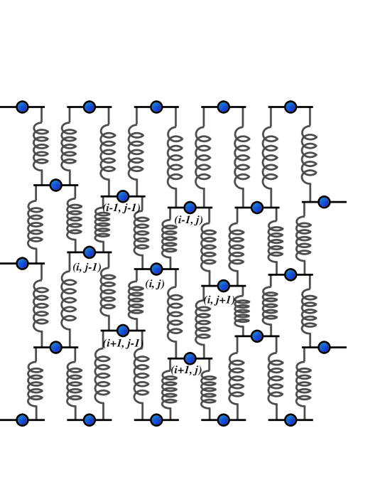
FIG. 1.: Elastic network considered in this paper. Each node is connected to two neighbors in the row above and to two neighbors in the row below, with movement confined to the vertical direction. A node $(i,j)$ and its surrounding nodes have been labeled. The system is compressed by holding the top and bottom rows each at fixed positions. Disorder in the stress distribution is introduced by variation of individual spring constants $k$. In the elastic regime, the $k$ values are chosen at random while in the granular regime, the $k$’s are additionally constrained so that the strain in each row is constant.

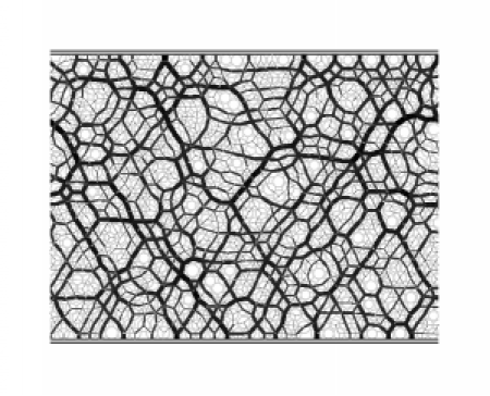
(a) $\Pi=0.1\Pi_{0}$

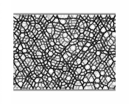
(b) $\Pi=\Pi_{0}$

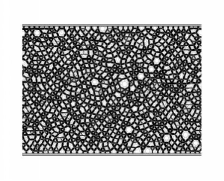
(c) $\Pi=10\Pi_{0}$

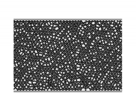
(d) $\Pi=50\Pi_{0}$

FIG. 2.: Contact networks of a sample MD-generated packing of 1024 discs for different values of applied external pressure $\Pi$. The reference pressure $\Pi_{0}$ is such that the average fractional change in particle radius at a contact is $6.25\times 10^{-4}$. In the transition from granular to elastic behavior, the number of contacts in the system increases and the magnitudes of the contact forces become more homogeneous. While the width of contacts shown is a proportional to the force magnitude, they have been rescaled for each pressure so direct comparisons between subfigures is not possible.

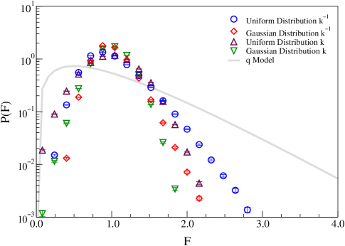
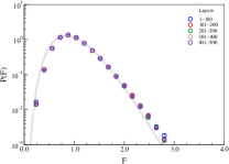
(a) Uniform $k^{-1}$ (b) Gaussian $k^{-1}$ (c) Uniform $k$ (d) Gaussian $k$

FIG. 3.: Force probability distribution $P(F)$ for 128-column random spring configurations. The form of $P(F)$ in the elastic regime depends on the distribution of spring constant values $k$. However, these $P(F)$ for all distributions of $k$ occupy a narrow range in comparison with the $q$-model granular regime result shown by the solid gray line. (a)-(d) We fit the functional form $P(F)\propto F^{A}e^{-BF}$ to the random $k^{-1}$ distributions with $A=6.67$ and $B=7.95$ for the uniform distribution and $A=14.70$ and $B=16.21$ for the gaussian distribution. For the random $k$ distributions, we fit $P(F)\propto e^{(F-1)^{2}/S^{2}}$ with $S=0.47$ for the uniform distribution and $S=0.32$ for the gaussian distribution. No differences are seen between layer groups near the edge or in the bulk of the systems.

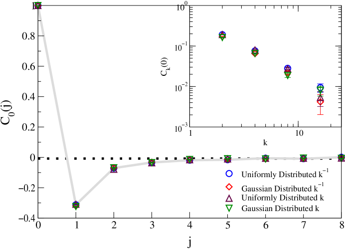
FIG. 4.: Spatial force-force correlation function $C_{k}(j)$ for the forces within the bulk layer grouping (layers 201-300) in 128-column elastic-regime scalar networks. In-plane correlations $C_{0}(j)$ are shown in the main plot while the vertical correlation peak decay given by $C_{k}(0)$ is shown in the inset. An observed nearest-neighbor in-plane anti-correlation appears to be robust with respect to variations in spring constant distributions. The vertical correlation is similarly robust.

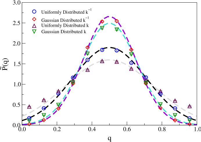
FIG. 5.: Force fraction probability distribution $\tilde{P}(q)$ within the bulk layer grouping (layers 201-300) for 128-column elastic-regime scalar networks. The fits are gaussians peaked at $q=0.5$ with the width being dependent on the spring constant distributions. Gaussian distributed $k^{-1}$ and $k$ configurations are narrower, with widths $\sigma\approx 0.16$ and $0.15$, respectively, than their uniformly distributed counterparts (random $k$, $\sigma\approx 0.25$ and random $k^{-1}$, $\sigma\approx 0.21$).

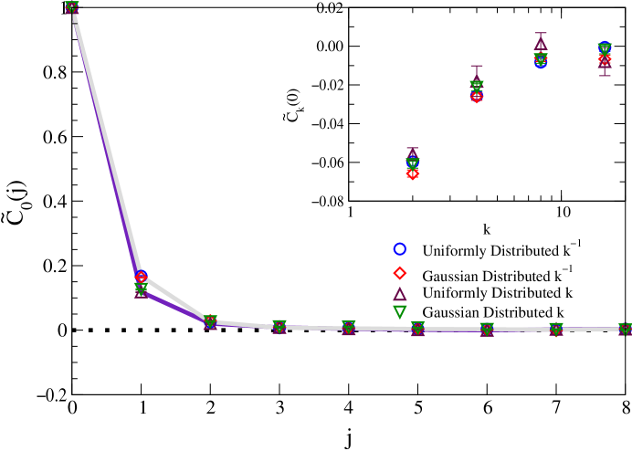
FIG. 6.: The two-point spatial correlation function $\tilde{C}_{k}(j)$ for the force fraction $q$ within the bulk layer grouping (layers 201-300) in 128-column elastic-regime scalar networks. In-plane correlations $\tilde{C}_{0}(j)$ are shown in the main plot with vertical correlations $\tilde{C}_{k}(0)$ in the inset. As with the force-force correlations, varying the spring constant distribution has minimal effect on these correlations.

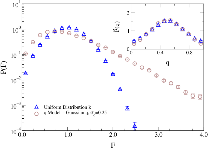
FIG. 7.: Effect of spatial correlation of $q$ values on the probability distribution of force $P(F)$. Force fraction probability distributions $\tilde{P}(q)$ of the uniform distribution of $k$ elastic network and a $q$-model system generated by choosing $q$ values from a gaussian distribution centered at $q=0.5$ with width $\sigma_{q}=0.25$ is shown in the inset. While the two $\tilde{P}(q)$ distributions appear nearly identical, the spatial correlations in the elastic network yield a functionally different form for the probability distribution of forces $P(F)$ than that of the uncorrelated $q$-model system.

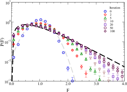
(a) $P(F)$ - Iterated scalar network

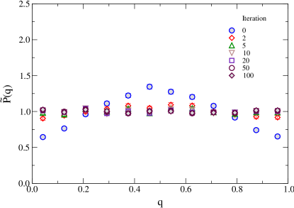
(b) $\tilde{P}(q)$ - Iterated scalar network

FIG. 8.: (a) Force probability distribution $P(F)$ at various stages of iteration for the bottom layer grouping (401-500) of an ensemble of 16-column scalar networks. Initially $P(F)$ is similar to the distribution for uniformly distributed $k$ systems, shown by the grey dashed line. The distribution broadens with increasing iterations with small $F$ agreement with granular $q$-model systems being achieved on order of 20 iterations. Further iterations are necessary to approach agreement for large values of $F$. The $P(F)$ distribution for $q$-model systems is shown by the black dashed line. (b) Force fraction probability distribution $\tilde{P}(q)$ at corresponding stages of iteration. The distribution of $q$ values approaches the expected uniform distribution within the first 10 iterations.

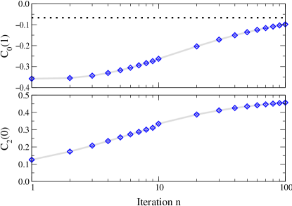
(a) Force-force correlations - Iterated scalar network

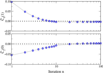
(b) $q$-$q$ correlations - Iterated scalar network

FIG. 9.: (a) Nearest-neighbor in-plane and vertical force-force correlation values $C_{0}(1)$ and $C_{2}(0)$ at various stages of iteration for an ensemble of 16-column scalar networks. The observed anti-correlation in nearest-neighbor forces decreases in magnitude as the number of iterations increases and appears to approach asymptotically the expected zero-correlation value. The vertical correlation increases in magnitude with increasing iterations, indicating a stronger preference for the formation of force vertical channels. (b) Nearest-neighbor in-plane and vertical $q$-$q$ correlation values $\tilde{C}_{0}(1)$ and $\tilde{C}_{2}(0)$. The spatial correlations for the force fraction $q$ decrease rapidly in magnitude as their values approach the uncorrelated target $q$ distribution.

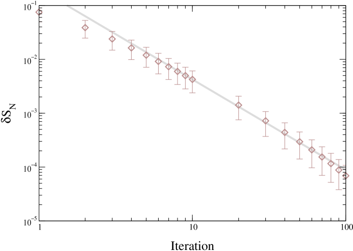
FIG. 10.: Deviation from constant strain $\delta{\mathcal{S}}_{N}$ for each layer in a scalar network system defined by Eq. 6. The solid line is a power law fit of form $\delta{\mathcal{S}}_{N}\propto n^{-\alpha}$ with $\alpha=-1.68\pm 0.02$. Increasing iterations confirm the approach to the constant strain limit, which is equivalent to the $q$ model.

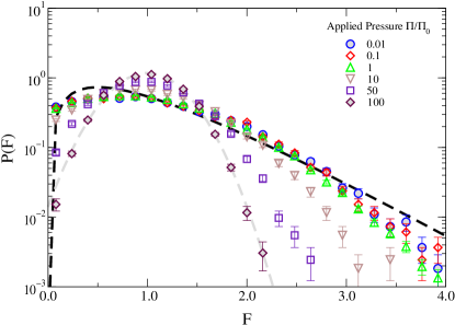
(a) $P(F)$ - MD packings at various applied pressures $\Pi$

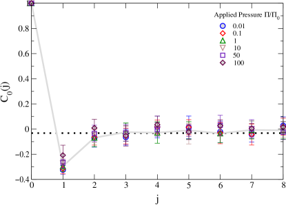
(b) $C_{0}(j)$ - MD packings at various applied pressures $\Pi$

FIG. 11.: (a) Progression of vertical force probability distribution $P(F)$ between elastic and granular regimes in MD-generated packings. At high applied pressure $\Pi$, $P(F)$ has a gaussian functional form, as shown by the gray dashed line, similar to the elastic behavior of the scalar network. At low pressure, $P(F)$ has widened and displays an exponential tail. For comparison, $P(F)$ for the $q$-model is shown by the black dashed line. The apparent transition to the granular regime appears to occur by roughly $\Pi/\Pi_{0}=1$. (b) In-plane force correlation function value $C_{0}(j)$ for various applied pressures. We define discs to be in-plane within a tolerance of $\pm 0.10a_{D}$ with spacings $j$ given in units of average disc diameter $2a_{D}$. Unlike the scalar networks, in the MD we see a consistent nearest-neighbor anti-correlation for all pressures.

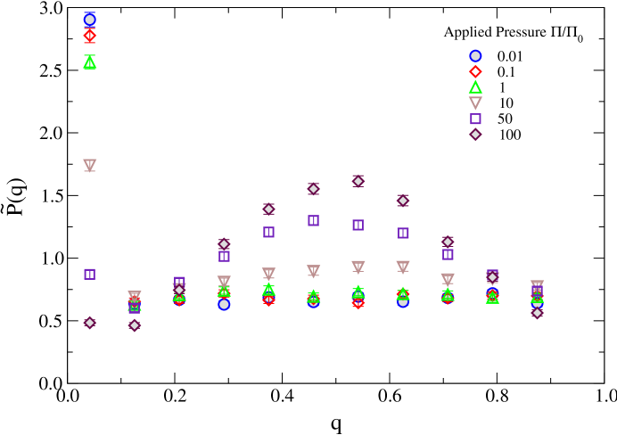
FIG. 12.: Progression of the vertical force fraction $q$ distribution $\tilde{P}(q)$ between elastic and granular regimes in MD-generated packings. Each $q$ is calculated as the fraction of the vertical force component that is transferred to the bottom left neighbors of a disc. At high pressures $\Pi$, we see a peaked form centered at $q=0.5$. For decreasing pressure, $\tilde{P}(q)$ flattens out and is roughly uniform. The increasing magnitude of the leftward bin with decreasing pressure $\Pi$ is due to increasing probability of isolated “rattlers” and discs with no bottom left neighbors.

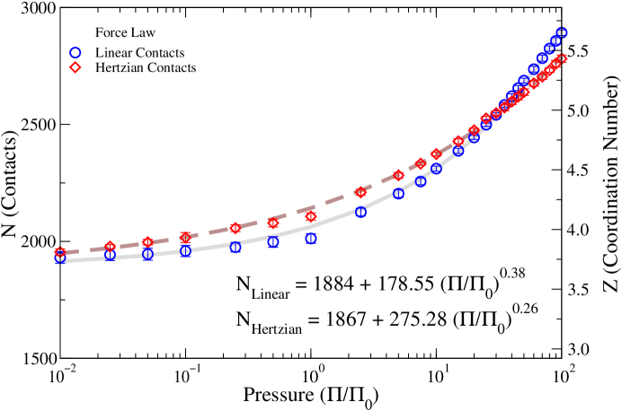
FIG. 13.: Number of contacts $N_{C}$ and coordination number $Z$ for MD-generated packings of 1024 discs versus externally applied pressure $\Pi$. The number of contacts fits roughly to a form $N_{C}=N_{0}+a(\Pi/\Pi_{0})^{b}$, where $N_{0}$ is the number of contacts in the zero-force limit. At low pressures, $N_{0}$ is slightly less than two contacts per particle because of the presence of “rattlers” in the zero-gravity system.

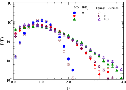
(a) $P(F)$ matches - scalar networks and MD packings

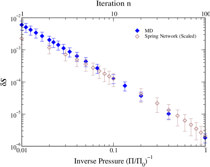
(b) Strain deviation $\delta{\mathcal{S}}$

FIG. 14.: (a) Matching vertical force probability distributions $P(F)$ for iterated scalar spring networks and MD packings of particles with a linear force law. We observe good agreement in the form of $P(F)$ between iteration $n=0$ and $\Pi/\Pi_{0}=100$, $n=10$ and $\Pi/\Pi_{0}=10$, $n=100$ and $\Pi/\Pi_{0}=1$. (b) Normalized strain deviation $\delta{\mathcal{S}}_{N}$ and $\delta{\mathcal{S}}_{MD}$ as a function of actual or equivalent applied pressure. The matching of $P(F)$ is used to generate a mapping between iteration values of the scalar networks and the pressures imposed on the MD systems. A simple scaling approach yields $\Pi_{\mathrm{eq}}/\Pi_{0}=100/n$. Additionally, $\delta{\mathcal{S}}_{N}$ for the scalar networks is scaled by a factor of 0.030 to achieve equivalence at $n=10$ ($\Pi/\Pi_{0}=10$).

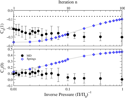
(a) Force correlations - MD and scalar networks

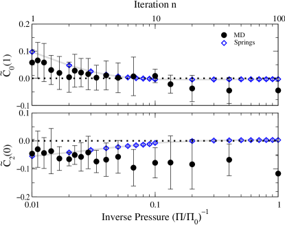
(b) $q$ correlations - MD and scalar networks

FIG. 15.: (a) Comparison of nearest-neighbor in-plane and vertical force-force correlation function values $C_{0}(1)$ and $C_{2}(0)$ between MD and scalar spring networks at various pressures $\Pi$ and iterations $n$. We see qualitative and quantitative differences in behavior. MD systems exhibit a significant in-plane nearest-neighbor anti-correlation throughout the crossover region. This contrasts with the decrease seen in the scalar networks as it approaches the granular limit (large iteration $n$). Strong vertical correlations develop in the scalar networks but not in the MD systems. (b) Nearest-neighbor in-plane and vertical $q$-$q$ correlation function values $\tilde{C}_{0}(1)$ and $\tilde{C}_{2}(0)$. The sizeable errors in the MD values allows for only qualitative comparisons. Both systems exhibit similar trends for in-plane nearest-neighbor correlation values. However, qualitative differences exist for the behavior of vertical correlations: the MD systems display a constant anti-correlation throughout the crossover region while the scalar networks exhibit an anti-correlation in the elastic regime which decays rapidly to uncorrelated behavior as the granular limit is approached.

REFERENCES

- [1] V. V. Sokolovskii, Statics of Granular Materials (Pergamon, Oxford, 1965).
- [2] R. M. Nedderman, Statics and Kinematics of Granular Materials (Cambridge University Press, Cambridge, 1992).
- [3] S. Edwards and R. Oakeshott, Physica D 38, 88 (1989).
- [4] J. P. Bouchaud, M. E. Cates, and P. Claudin, J. Phys. I France 5, 639 (1995).
- [5] J. P. Wittmer, M. E. Cates, and P. Claudin, J. Phys. I France 7, 39 (1997).
- [6] The non-tensile constraint and the incompressibility are approximate; for example, cohesive forces arise from capillary condensation (see D. Hornbaker et al., Nature 387, 765 (1997); R. Albert et al., Phys. Rev. E 56, R6271 (1997); T. Halsey and A. Levine, Phys. Rev. Lett. 80, 3141 (1998); and L. Bocquet, E. Charlaix, S. Ciliberto, and J. Crassous, Nature 396, 735 (1998).), and all materials deform in response to an applied stress. However, these approximations are very good in many dry granular media.
- [7] J. P. Wittmer, P. Claudin, M. E. Cates, and J.-P. Bouchaud, Nature 382, 336 (1996).
- [8] M. E. Cates et al., Phys. Rev. Lett. 81, 1841 (1998).
- [9] A. V. Tkachenko and T. A. Witten, Phys. Rev. E 60, 687 (1999).
- [10] C. Liu et al., Science 269, 513 (1995).
- [11] S. N. Coppersmith et al., Phys. Rev. E 53, 4673 (1996).
- [12] In particular, it does not describe well the long-wavelength properties of stress transmission. Vector generalizations that aim to capture these properties accurately include C. Eloy and C. Clément, J. Phys. I France 7, 1541 (1997); J. E. S. Socolar, Phys. Rev. E 57, 3204 (1998); P. Claudin, J.-P. Bouchaud, M. E. Cates, and J. P. Wittmer, Phys. Rev. E 57, 4441 (1998); and M. L. Nguyen and S. N. Coppersmith, Phys. Rev. E 59, 5870 (1999).
- [13] B. Miller, C. O’Hern, and R. P. Behringer, Phys. Rev. Lett. 77, 3110 (1996).
- [14] G. W. Baxter, in Powders and Grains 97, edited by R. P. Behringer and J. T. Jenkins (Balkena, Rotterdam, 1997), pp. 345–348.
- [15] D. M. Mueth, H. M. Jaeger, and S. R. Nagel, Phys. Rev. E 57, 3164 (1998).
- [16] F. Radjai, M. Jean, J. J. Moreau, and S. Roux, Phys. Rev. Lett. 77, 274 (1996).
- [17] F. Radjai, D. Wolf, M. Jean, and J. J. Moreau (unpublished).
- [18] F. Radjai et al., in Powders and Grains 97, edited by R. P. Behringer and J. T. Jenkins (Balkena, Rotterdam, 1997), pp. 211–214. See Ref. [14].
- [19] S. Luding, Phys. Rev. E 55, 4720 (1997).
- [20] R. Clelland (unpublished).
- [21] C. Thornton and S. J. Antony, Phil Trans Roy Soc A 356, 2763 (1998).
- [22] W. Tang and M. Thorpe, Phys. Rev. B 36, 3798 (1987).
- [23] W. Tang and M. Thorpe, Phys. Rev. B 37, 5539 (1988).
- [24] E. Guyon et al., Reports on Progress in Physics 53, 373 (1990).
- [25] M. G. Sexton, J. E. S. Socolar, and D. G. Schaeffer, Phys. Rev. E 60, 1999 (1999).
- [26] M. Sahimi, Phys. Rep. 306, 214 (1998).
- [27] P. Bamberg and S. Sternberg, A Course in Mathematics for Students of Physics (Cambrige University Press, Cambridge, 1990), Vol. 2, pp. 407–457.
- [28] M. Nicodemi, Phys. Rev. Lett. 80, 1340 (1998).
- [29] D. J. Durian, Phys. Rev. Lett. 75, 4780 (1995).
- [30] D. J. Durian, Phys. Rev. E 55, 1739 (1997).
- [31] S. J. Langer and A. J. Liu, J Phys Chem B 101, 8667 (1997).
- [32] L. D. Landau and E. M. Lifshitz, Theory of Elasticity, Vol. 7 of Course of Theoretical Physics, 3rd ed. (Butterworth-Heinemann, Oxford, 1986).
- [33] J. Krug and J. Garcia, cond-mat/9909034 (unpublished).
- [34] R. R. Majumdar and S. N. Majumdar, cond-mat/9910206 (unpublished).
- [35] This matching between iteration number and pressure applies for polydisperities greater than roughly . The behavior of in nearly monodisperse 2-D systems, where large regions of crystallization are present, is currently under investigation (M. L. Nguyen, unpublished).
- [36] D. Howell, R. P. Behringer, and C. Veje, Phys. Rev. Lett. 82, 5241 (1999).
- [37] H. A. Makse, D. L. Johnson, and L. M. Schwartz, cond-mat/0002102 (unpublished).
- [38] P. Claudin and J.-P. Bouchaud, Phys. Rev. Lett. 78, 231 (1997).