Universality and nonmonotonic finite-size effects above the upper critical dimension

Abstract

We analyze universal and nonuniversal finite-size effects of lattice systems in a $L^{d}$ geometry above the upper critical dimension $d=4$ within the O$(n)$ symmetric $\varphi^{4}$ lattice theory. On the basis of exact results for $n\rightarrow\infty$ and one-loop results for $n=1$ we identify significant lattice effects that cannot be explained by the $\varphi^{4}$ continuum theory. Our analysis resolves longstanding discrepancies between earlier asymptotic theories and Monte Carlo (MC) data for the five-dimensional Ising model of small size. We predict a nonmonotonic $L$ dependence of the scaled susceptibility $\chi L^{-d/2}$ at $T_{c}$ with a weak maximum that has not yet been detected by MC data.

The concept of universality plays a fundamental role in statistical and elementary particle physics [1, 2]. It implies that a unifying description of various physically different lattice and continuum systems near criticality can be given within the $\varphi^{4}$ field theory with the Hamiltonian

$$H=\int d^{d}x\left[\frac{r_{0}}{2}\;\varphi^{2}+\frac{1}{2}(\nabla\varphi)^{2}+u_{0}\;{(\varphi^{2})}^{2}\right]\;.$$ (1)

The wide applicability of this theory is well established below the upper critical dimension $d^{*}=4$ [1, 2]. Particular accuracy has been achieved in testing the universal predictions of the $\varphi^{4}$ theory by means of numerical data for the universality class of the $d=3$ Ising model not only for bulk properties but also for finite-size effects with periodic boundary conditions (p.b.c.) [3, 4, 5].

Less well established, however, is the range of applicability of the $\varphi^{4}$ theory for confined systems $\it{above}$ the upper critical dimension where the critical exponents are mean-field like [1, 2]. Early disagreements between Monte Carlo (MC) data for the finite $d=5$ Ising model [6] and universal predictions based on $H$ [4] have led to a longstanding debate [7]. New discrepancies between accurate MC data [8] and recent quantitative finite-size scaling predictions [9] based on the $\varphi^{4}$ lattice Hamiltonian

$$\hat{H}=\sum_{i}\left[\frac{r_{0}}{2}\varphi^{2}_{i}+u_{0}(\varphi^{2}_{i})^{2}\right]+\sum_{<ij>}\frac{J}{2}(\varphi_{i}-\varphi_{j})^{2}$$ (2)

have raised the question to what extent the $\varphi^{4}$ theory is capable of describing finite-size effects of the Ising model for $d>4$. In particular the recently discovered [9, 10] non-equivalence of $H$ and $\hat{H}$ for finite systems is in striking contrast to the situation for $d<4$. This non-equivalence may be relevant not only for higher-dimensional finite systems but also for three-dimensional physical systems for which mean-field theory provides a good description, such as systems with long but finite range interactions [11], polymer mixtures near their critical point of unmixing [12], and systems with a tricritical point [13].

In this Letter we resolve the existing discrepancies for $d>4$ on the basis of exact results for the O$(n)$ symmetric $\varphi^{4}$ theory in the limit $n\rightarrow\infty$ and of one-loop results for $n=1$. Our analysis of both $\hat{H}$ and $H$ with a smooth and a sharp cutoff is not restricted to large $L$ and allows us to specify the range of validity of universal finite-size scaling for p.b.c. in a $L^{d}$ geometry. We find, for p.b.c., that $H$ with a smooth cutoff belongs to the same universality class as $\hat{H}$ whereas $H$ with a sharp cutoff exhibits different nonuniversal finite-size effects. This implies that the lowest-mode prediction [4] of universal ratios at $T_{c}$ for $d>4$ is indeed valid asymptotically for both the lattice $\varphi^{4}$ theory and the continuum $\varphi^{4}$ theory with a smooth cutoff. We demonstrate, however, that the existing MC data for the $d=5$ Ising model of small size [6, 7, 8] are outside the asymptotic scaling regime and cannot be explained by $H$ because of significant lattice effects. We also demonstrate that our one-loop results based on $\hat{H}$ are in quantitative agreement with the MC data [8] for $4\leq L\leq 22$ and that the one-loop two-variable scaling results [9, 14] are well applicable to $L\gtrsim 12$, contrary to earlier conclusions [8, 15]. We predict a weak maximum of the $L$-dependence of the scaled susceptibility $\chi L^{-d/2}$ at $T_{c}$ which has not yet been detected in the MC data [8]. Our analysis implies $\xi_{0}=0.396$ for the bulk correlation-length amplitude of the $d=5$ Ising model, in disagreement with $\xi_{0}=0.549$ found in Ref. [8].

We start from $\hat{H}$, Eq.(2), for the $n$-component variables $\varphi_{i}$ on a finite sc lattice of volume $L^{d}$ with a nearest-neighbor coupling $J>0$. The basic question is to what extent $\hat{H}$ is equivalent to the spin Hamiltonian $H_{s}=-K\;\sum_{<ij>}s_{i}\;s_{j}$ where the $n$-component spin variables have a fixed length $s^{2}_{i}=n$, in contrast to $\varphi_{i}$ whose components $\varphi_{i\alpha}$ vary in the range $-\infty\leq\varphi_{i\alpha}\leq\infty$. For $n=1,H_{s}$ is the Ising Hamiltonian with $s_{i}=\pm\;1$ and $K>0$.

An exact equivalence between $\hat{H}$ and $H_{s}$ exists in the limit $u_{0}\rightarrow\infty$, $r_{0}\rightarrow-\infty$ at fixed $u_{0}/(Jr_{0})$ for general $L$, $n$ and $d$. Choosing $u_{0}/(Jr_{0})$ such that $K=-Jr_{0}/(4u_{0}n)$ we obtain by means of a saddle-point integration

$$\lim_{u_{0}\rightarrow\infty\atop-r_{0}\rightarrow\infty}\chi=\;\frac{K}{J}\;\;\chi_{s}$$ (3)

where $\chi$ and $\chi_{s}$ are the susceptibilities

$$\chi = (nL^{d})^{-1}\;\sum_{i,j}<\varphi_{i}\;\varphi_{j}>\;,$$ (4)

$$\chi_{s} = (nL^{d})^{-1}\;\sum_{i,j}\;<s_{i}\;s_{j}>\;.$$ (5)

The weights in Eqs. (4) and (5) are $e^{-\hat{H}}$ and $e^{-H_{s}}$, respectively. For $n=1$, this exact equivalence is of limited relevance since all calculations within the $\varphi^{4}$ model are performed at finite $u_{0}$. Hence, even in an exact theory, we have $\chi_{s}\neq J\chi/K$ at finite $u_{0}$. Therefore, in a quantitative comparison of $\chi$ with MC data for $\chi_{s}$, one must allow for a ($T$ and $L$ independent) overall amplitude $A$ which is adjusted such that $\chi_{s}=AJ\chi/K$. For finite $u_{0}$, the constant $A$ accounts for an appropriate normalization of the variables $\varphi_{i}$ relative to the discrete variables $s_{i}=\pm 1$. In an approximate theory, the value of $A$ depends on the approximations made for $\chi$. This corresponds to an adjustment merely of the nonuniversal bulk amplitude and not of the $L$ dependence of $\chi$ (for $d=3$ see, e.g., Ref.[5]). An adjustment of $A$ was not taken into account in the analysis of Ref. [8].

Of particular interest is the case $n\rightarrow\infty$ since it provides the opportunity of studying the exact $u_{0}$ dependence including $u_{0}\rightarrow\infty$. This reveals the structural similarity between $\chi$ at finite $u_{0}$ and at $u_{0}=\infty$. This is most informative for $d>4$ where the leading and subleading powers of $L$ are independent of $n$ and should apply also to the Ising universality class with $n=1$.

For $n\rightarrow\infty$ at fixed $u_{0}n$ the susceptibility $\hat{\chi}=2J\chi$ for p.b.c. is determined implicitly by [10]

$$\hat{\chi}^{-1}=\;r_{0}/(2J)\;+\;J^{-2}u_{0}n\;L^{-d}\sum_{\bf k}G_{\bf k}(\hat{\chi}^{-1}),$$ (6)

with $G_{\bf k}(\hat{\chi}^{-1})=(\hat{\chi}^{-1}+J_{\bf k})^{-1}$ and $J_{\bf k}=2\sum^{d}_{j=1}(1-\cos k_{j})$ where $\sum_{\bf k}$ runs over $\bf k$ vectors with components $k_{j}=2\pi m_{j}/L,\;m_{j}=0,\pm 1,\pm 2...,j=1,2,...,d$ in the range $-\pi\leq k_{j}<\pi$. At $T=T_{c}$ we derive from Eq. (6) the exact implicit equation for $d>4$

$$\hat{\chi}^{2}=L^{d}\;\;\frac{\lambda_{0}(u_{0})-\hat{\chi}^{(4-d)/2}\;f_{b}\;(\hat{\chi}^{-1})}{1-L^{d}\;\;\hat{\chi}^{-1}\;\hat{\Delta}_{1}(\hat{\chi}^{-1},\;L)}$$ (7)

with $\lambda_{0}(u_{0})=\;(J^{2}+u_{0}n\;\int\limits_{\bf k}J_{\bf k}^{-2})\;(u_{0}n)^{-1}$ and

$$f_{b}(\hat{\chi}^{-1}) = \hat{\chi}^{(d-6)/2}\int\limits_{\bf k}\left[J_{\bf k}^{2}(\hat{\chi}^{-1}+J_{\bf k})\right]^{-1},$$ (8)

$$\hat{\Delta}_{m}(\hat{\chi}^{-1},L) = \int\limits_{\bf k}G_{\bf k}(\hat{\chi}^{-1})^{m}-L^{-d}\sum_{{\bf k}\neq{\bf 0}}G_{\bf k}(\hat{\chi}^{-1})^{m},$$ (9)

where $\int_{\bf k}\equiv(2\pi)^{-d}\int d^{d}\;k$ with $|k_{j}|\leq\pi$. We see that the structure of the $L$ dependence of $\hat{\chi}$ for finite $u_{0}>0$ is the same as for $u_{0}\rightarrow\infty$ where $\lambda_{0}(u_{0})$ is reduced to $\lambda_{0}=\int_{\bf k}J_{\bf k}^{-2}$. It is reasonable to expect that also for $n=1$ the calculation of $\hat{\chi}$ at finite $u_{0}$ yields essentially the correct structure of $\chi_{s}$.

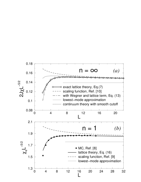
FIG. 1.: Scaled susceptibilities for $d=5$ at $T_{c}$. Solid and dashed lines approach the lowest-mode lines for $L\rightarrow\infty$.

In Fig. 1a we show the exact result of $\hat{\chi}L^{-5/2}$ for $n\rightarrow\infty$ and $d=5$ at $T_{c}$ by solving Eq. (7) numerically with $\lambda_{0}=\int_{\bf k}J_{\bf k}^{-2}=0.01935$. We find that $\hat{\chi}L^{-5/2}$ has a weak maximum at $L=9$ which is not contained in the (large $L$) scaling form $\hat{\chi}_{scal}=L^{d/2}\;\tilde{P}(L^{4-d}/\lambda_{0})$ of Ref. [10] (dashed curve). In $\hat{\chi}_{scal}$ the nonasymptotic Wegner correction $\propto f_{b}$ was neglected and $\hat{\Delta}_{1}$ was approximated only by the leading term $\hat{\Delta}_{1}=I_{1}(\hat{\chi}^{-1}\;L^{2})\;L^{2-d}$ with

$$I_{m}(x)=\int^{\infty}_{0}dt\;{t^{m-1}[K_{b}(t)^{d}-K(t)^{d}+1]\over(2\pi)^{2m}e^{(xt/4\pi^{2})}},$$ (10)

where $K_{b}(t)=(\pi/t)^{1/2}$ and $K(t)=\sum^{\infty}_{j=-\infty}\exp(-j^{2}t)$. Both $\hat{\chi}$ and $\hat{\chi}_{scal}$ show the predicted [9] slow $O(L^{(4-d)/2})$ approach to the large-$L$ limit $\hat{\chi}_{0}L^{-d/2}=\lambda^{1/2}_{0}$ corresponding to the lowest-mode approximation (horizontal line in Fig. 1a). Note that both $\hat{\chi}$ and $\hat{\chi}_{scal}$ approach $\hat{\chi}_{0}$ from above.

The small difference between $\hat{\chi}$ and $\hat{\chi}_{scal}$ in Fig. 1a for $L\gtrsim 15$ arises from the negative Wegner correction term $-\hat{\chi}^{(4-d)/2}f_{b}(\hat{\chi}^{-1})\propto-L^{(4-d)d/4}f_{b}(0)$ in the numerator of Eq. (7). The pronounced departure of $\hat{\chi}$ from $\hat{\chi}_{scal}$ for $L\lesssim 10$, however, is a lattice effect that is dominated by the subleading term $-\hat{M}_{1}L^{-d}$ in

$$\hat{\Delta}_{1}(\hat{\chi}^{-1},L)=I_{1}(x)L^{2-d}-\hat{M}_{1}(x)L^{-d}+O(L^{-d-2})$$ , (11)

$$\hat{M}_{1}(x)=\int^{\infty}_{0}dt\;{[K(t)^{d-1}K^{\prime\prime}(t)-K_{b}(t)^{d-1}K^{\prime\prime}_{b}(t)]\over e^{(xt/4\pi^{2})}}$$ , (12)

with $x=\hat{\chi}^{-1}L^{2}$. Unlike the leading term $I_{1}L^{2-d}$, the lattice term $-\hat{M}_{1}L^{-d}$ cannot be incorporated in the universal finite-size scaling function $\tilde{P}(y)$ which depends on $y=(L/l_{0})^{4-d}$ with $l_{0}^{4-d}=\lambda_{0}$. In summary, the leading $L$ dependence of $\hat{\chi}$ is represented as

$$\hat{\chi}=\left(\lambda_{0}L^{d}\frac{1\;-\;q_{2}L^{(4-d)d/4}}{1-q_{1}L^{(4-d)/2}+q_{3}L^{-d/2}}\right)^{1/2}$$ (13)

where $q_{1}=\lambda_{0}^{-1/2}I_{1}(x),\;q_{2}=\lambda_{0}^{-d/4}\;f_{b}(0)$, and $q_{3}=\lambda_{0}^{-1/2}\hat{M}_{1}(x)$. The functions $I_{1}(x)$ and $\hat{M}_{1}(x)$ have a weak $x$ dependence with $I_{1}(0)=0.107$ and $\hat{M}_{1}(0)=0.676$ for $d=5$. Eq. (13) is shown in Fig. 1a as dot-dashed line which approximates the exact result, Eq. (7), with very good accuracy down to $L=3$.

Now we turn to the question to what extent $H$, Eq. (1), is equivalent to $\hat{H}$. From our result of $\hat{\chi}$, Eqs. (6) - (9), we obtain the corresponding result of $\chi_{field}=n^{-1}\int d^{d}x<\varphi(x)\varphi(0)>$ after replacing $J_{\bf k}$ by $k^{2}$ and setting $2J=1$. A novel feature for $d>4$ is the fact that $\Delta_{1}$ depends significantly on the cutoff procedure. We need to distinguish two cases : (a) a sharp cutoff $\Lambda$ which restricts the $\bf k$ vector to $|k_{j}|\leq\Lambda$, (b) a smooth cutoff $\Lambda$ where $-\infty\leq k_{j}\leq\infty$ but where $(\hat{\chi}^{-1}+k^{2})^{-m}$ is replaced by the (Schwinger type) regularized form [2] $(\hat{\chi}^{-1}+k^{2})^{-m}_{reg}=\int^{\infty}_{\Lambda^{-2}}ds\;s^{m-1}\;\exp\;[-(\hat{\chi}^{-1}+k^{2})s]$. The former case (a) implies [9, 10] $\Delta_{1}\propto L^{-2}$ and $\chi_{field}\propto L^{d-2}$ at $T_{c}$ which differs fundamentally from the lattice result $\hat{\chi}\propto L^{d/2}$. In the latter case (b), however, Eqs. (11) and (12) are replaced by

$$\Delta_{1}(\hat{\chi}^{-1},L) = I_{1}(x)L^{2-d}-M_{1}(\hat{\chi}^{-1})L^{-d}+O(e^{-\Lambda^{2}L^{2}}),$$ (14)

$$M_{1}(\hat{\chi}^{-1}) = \hat{\chi}[1-\exp(-\hat{\chi}^{-1}\Lambda^{-2})],$$ (15)

with the same leading term $I_{1}L^{2-d}$. This implies that $\chi_{field}$ with a smooth cutoff has the same asymptotic (large $L$) finite-size scaling behavior as $\hat{\chi}_{scal}$. Adjustment of the leading amplitude $\lambda_{0}^{field}=\int_{\bf k}(k^{-2})^{-2}_{reg}$ to the lattice counterpart $\lambda_{0}=\int_{\bf k}J_{\bf k}^{-2}$ fixes the cutoff as $\Lambda=0.185$ and $M_{1}(0)=\Lambda^{-2}=0.034$ for $d=5$ which is smaller than $\hat{M}_{1}(0)$ by a factor of 20. This difference between $\hat{M}_{1}$ and $M_{1}$ constitutes a significant lattice effect for small $L$ that is exhibited in Fig. 1a, with $\chi_{field}\;L^{-5/2}$ represented by the dotted line. We conclude that $H$ with a smooth cutoff yields the same (large $L$) finite-size scaling behavior as $\hat{H}$ (for cubic geometry and p.b.c.) but does not account for the strong $L$-dependence of $\hat{\chi}L^{-d/2}$ for small $L$. We expect this conclusion to hold for general $n$.

Now we consider $\hat{H}$ for the relevant case $n\;=\;1$. We start from the one-loop result for $\hat{\chi}=2J\chi$ and for the ratio $Q=<\Phi^{2}>^{2}/<\Phi^{4}>$ of moments $<\Phi^{m}>$ for the order parameter distribution where $\Phi=L^{-d}\;\Sigma_{j}\;\varphi_{j}$. The analytic result reads for arbitrary $L$ [9]

$$\hat{\chi} = L^{d/2}\;{(u_{0}^{eff})^{-1/2}}\;\vartheta_{2}\;(Y^{eff}),$$ (16)

$$Q = \vartheta_{2}(Y^{eff})^{2}\;/\;\vartheta_{4}(Y^{eff}),$$ (17)

$$Y^{eff} = L^{d/2}\;r_{0}^{eff}(u_{0}^{eff})^{-1/2},$$ (18)

$$\vartheta_{m}(Y) = {\int^{\infty}_{0}dss^{m}\exp\left(-{1\over 2}Ys^{2}-s^{4}\right)\over\int^{\infty}_{0}ds\exp\left(-{1\over 2}Ys^{2}-s^{4}\right)}$$ (19)

with the effective parameters

$$r_{0}^{eff} = \tilde{a}_{0}t+12\tilde{u}_{0}(S_{1}-\lambda_{0})+144\;\tilde{u}_{0}^{2}M_{0}^{2}S_{2},$$ (20)

$$u_{0}^{eff} = \tilde{u}_{0}-36\tilde{u}_{0}^{2}S_{2},$$ (21)

$$S_{m} = L^{-d}\sum_{{\bf k}\neq{\bf 0}}(\tilde{a}_{0}t+12\tilde{u}_{0}M_{0}^{2}+J_{\bf k})^{-m},$$ (22)

$$M_{0}^{2} = (L^{d}\;\tilde{u}_{0})^{-1/2}\;\vartheta_{2}(L^{d/2}\;\tilde{a}_{0}t\;\tilde{u}_{0}^{-1/2})\;.$$ (23)

The r.h.s. of Eqs. (16) - (23) depend only on the parameters $\tilde{u}_{0}=u_{0}/(4J^{2})$ and $\tilde{a}_{0}=a_{0}/(2J)$ where $a_{0}=(r_{0}-r_{0c})/t$ with $t=(T-T_{c})/T_{c}$. Eqs. (16) - (23) were evaluated previously [9] only for large $L$. Here we present the numerical evaluation of Eqs. (16) - (23) for arbitrary $L\leq 32$ without further approximation for $d=5$ including Wegner corrections and lattice terms. Our strategy of adjusting $\tilde{u}_{0}$ is based on the fact that $Q$ at $T=T_{c}$ depends only on $\tilde{u}_{0}$ and that no overall adjustment for $Q$ is required since $\lim_{L\rightarrow\infty}Q=Q_{0}$ is universal. Thus we adjust $\tilde{u}_{0}=0.93$ to the MC data [8] of $Q$ at $T_{c}$ (Fig. 2), then we use the same $\tilde{u}_{0}$ for $\hat{\chi}$ at $T_{c}$. For the comparison of $\hat{\chi}$ with the MC data for $\chi_{s}$ at $T_{c}$ we introduce the amplitude $A$ according to $\chi_{s}=AJ\chi/K=A\hat{\chi}/(2K_{c})$. Using [8] $K_{c}=0.1139155$ and adjusting $A=0.678$ yields the solid line in Fig. 1b. At $T\neq T_{c}$ we determine $\tilde{a}_{0}=2.87$ from the bulk susceptibility $\chi_{s}=1.322t^{-1}$ of series expansion results [16].

In Figs. 1b-3 our analytic result (solid lines) is compared with the MC data of Ref. [8]. We conclude that our one-loop finite-size theory based on $\hat{H}$ satisfactorily describes the existing MC data for $4\leq L\leq 22$, both at $T_{c}$ and away from $T_{c}$ (Fig.3). We attribute the remaining deviations of $Q$ for small $L$ to the (expected) inaccuracy of our one-loop approximation. At $T=T_{c}$ our analytic results approach the lowest-mode results $\lim_{L\rightarrow\infty}\chi_{s}L^{-5/2}=p_{0}=1.757$ and $Q_{0}=0.4569$ (horizontal lines in Figs. 1b and 2) from above, in particular our theory predicts a (weak) maximum of $\chi_{s}L^{-5/2}$ at $T_{c}$ (similar to that in Fig. 1a for $n=\infty$) that has not yet been detected in the MC data [8]. Our theory also predicts a nonmonotonic $L$ dependence of $Q$ at $T_{c}$ (Fig. 2) and of the scaled magnetization $<|\Phi|>L^{5/4}$ at $T_{c}$.

Finally we answer the question to what extent the MC data in Figs. 1b-3 can be described by the finite-size scaling forms of $\hat{\chi}_{scal}=2J\chi_{scal}$ and $Q_{scal}$ derived previously (Eqs. (76) - (88) of Ref. [9]) on the basis of $\hat{H}$. These scaling forms neglect Wegner corrections and lattice effects. We have found that the same scaling functions can be derived on the basis of $H$ provided that a smooth cutoff is used. The corresponding scaling functions depend on the two scaling variables $x=t(L/\xi_{0})^{2}$ and $y=(L/l_{0})^{4-d}$ where $\xi_{0}\propto\tilde{a}_{0}^{-1/2}$ is the amplitude of the bulk correlation length and $l_{0}\propto\tilde{u}_{0}^{1/(d-4)}$ is a second reference length. Thus, instead of $\tilde{u}_{0}$ and $\tilde{a}_{0}$, we now have $l_{0}$ and $\xi_{0}$ as adjustable parameters. Since the one-loop results for $\hat{\chi}$ and $\hat{\chi}_{scal}$ differ at $O(\tilde{u}_{0}^{2})$ one must allow for a different amplitude $A_{scal}\neq A$ in the adjustment of $\hat{\chi}_{scal}$ to $\chi_{s}$. Using the same strategy of adjustment as described above we find $l_{0}=2.641$ from $Q$ at $T_{c}$ and $A_{scal}=1.925$ from $\chi_{s}=A_{scal}\hat{\chi}_{scal}/(2K_{c})$. Finally we determine $\xi_{0}=0.396$ from the one-loop bulk result $\lim_{t\rightarrow 0}\lim_{L\rightarrow\infty}\chi_{s}t=A_{scal}\xi_{0}^{2}/(2K_{c})=1.322$. The corresponding scaling results are shown in Figs. 1b-3 as dashed lines. We identify the significant departure of the MC data for $\chi_{s}$ at $T_{c}$ from the dashed line for $L\lesssim 12$ as a lattice effect that is well described by our full one-loop theory (solid line in Fig. 1b) but which is not captured by the scaling form.

FIG. 2.: Moment ratio $Q$ at $T_{c}$ for $d=5$ and $n=1$. Solid and dashed lines approach the lowest-mode line for $L\rightarrow\infty$.

FIG. 3.: Temperature dependence of susceptibilities for $d=5$ and $n=1$: $10^{-2}\chi_{s}$ for $L=4$ and $10^{-3}\chi_{s}$ for $L=12$ .

This failure of the scaling form for $L\lesssim 12$ was first observed by Luijten et al.[8]. We see, however, that there is good agreement of our scaling results with the MC data for $L\gtrsim 12$, contrary to the disagreement found in Ref.[8]. The latter disagreement is due to the (unjustified) identification [8] $J=K,\chi_{s}=\chi$ corresponding to $A_{scal}=1$ which, together with the fitting formula Eq.(32) of Ref.[8], implied $\xi_{0}=0.549$ and $l_{0}=0.603$. This formula omits the leading Wegner correction $\propto L^{(4-d)d/4}$ and a negative lattice term $\propto L^{-d/2}$ [compare our Eq.(13)] and therefore implies an increasing $\chi_{s}L^{-5/2}$ (Fig. 9 of Ref.[8]) towards $\lim_{L\rightarrow\infty}\chi_{s}L^{-5/2}=p_{0}=1.91$, in contrast to the decreasing $\chi_{s}L^{-5/2}$ with $p_{0}=1.76$ of our one-loop theory. More accurate MC data would be desirable which could distinguish between our quantitative predictions in Figs. 1b and 2 and those implied by the analysis of Ref.[8]. It would also be desirable to determine $\xi_{0}$ for the $d=5$ Ising model (e.g. from series expansion results) in order to resolve the disagreement between our prediction for $\xi_{0}$ and that of Ref.[8].

We thank K. Binder, H.W.J. Blöte and E. Luijten for providing us with their MC data in numerical form. Support by Sonderforschungsbereich 341 der DFG and by NASA is acknowledged. One of us (X.S.C.) thanks the NSF of China for support under Grant No. 19704005.