Noise in neurons is message-dependent
(neuronal reliability/temporal coding/information theory/error-correcting)

Abstract

Neuronal responses are conspicuously variable. We focus on one particular aspect of that variability: the precision of action potential timing. We show that for common models of noisy spike generation, elementary considerations imply that such variability is a function of the input, and can be made arbitrarily large or small by a suitable choice of inputs. Our considerations are expected to extend to virtually any mechanism of spike generation, and we illustrate them with data from the visual pathway. Thus, a simplification usually made in the application of information theory to neural processing is violated: noise is not independent of the message. However, we also show the existence of error-correcting topologies, which can achieve better timing reliability than their components.

I Introduction

Brains represent signals by sequences of identical action potentials or spikes [1]. Upon presentation of a stimulus, a given neuron will produce a certain pattern of spikes; upon repeating the stimulus, the pattern may repeat spike for spike in a highly reliable fashion, or may be similar only ”rate-wise”, or some spikes may be repeatable and others not. If individual spikes can be recognized and tracked across trials, then their timing accuracy can be ascertained unambiguously; this is not always the case. The existence of repeatable spike patterns and the reliability of their timing changes not only from neuron to neuron, but even for the same neuron under varying circumstances. Bryant and Segundo [2] first noticed (in the mollusk Aplysia) that spike timing accuracy depends on the particulars of the input driving the neuron. This intriguing property has received renewed attention, notably among those searching for experimental evidence supporting different theories of neural coding [3, 4]. In a study of the response of pyramidal neurons to injected current [3] the temporal pattern of firing was found to be unreliable when the injected current was constant, but highly reliable when the input current was “noisy” and contained high frequency components. This study showed explicitly the difference between the irregularity of the spike pattern (which was irregular in both cases) as opposed to the reliability or accuracy of spike timing, and also highlighted the connection that “natural” stimuli are noisy and contain sharp transitions. Similar results have been obtained from in vivo recordings of the H1 neuron in the visual system of the fly [4]: constant stimuli produced unreliable or irreproducible spike firing patterns, but noisy input signals deemed to be more “natural” and representative of a fly in flight yielded much more reproducible spike patterns, in terms of both timing and counting precision. Although some aspects of the last study have been challenged recently in [5], the phenomenon of different reliabilities for varying inputs was reaffirmed: see e.g. Fig. 1 in [5]. Thus one concludes that similar observations of the timing precision of spikes can be made in very different types of neurons under vastly different conditions, and that this must be a very universal, almost basic characteristic of neuronal function. We shall now show how these experimental observations follow from rather general and elementary considerations, and discuss the possible implications for brain function and architecture.

II Stochastic spiking models

The essence of this phenomenon can be demonstrated easily in toy models. A simple example is the leaky integrate-and-fire (I-F) model [6], which assumes the neuron is a (leaky) capacitor driven by a current which simulates the actual synaptic inputs. We add membrane fluctuations representing several internal sources of noise (cluttering of ion channels, synaptic noise, etc.) to obtain a system described by the following Langevin [7] equation:

$$C\dot{V}=-gV+I(t)+\xi(t)$$ (1)

where $C$ is the cell membrane capacitance, $V$ the membrane potential, $gV$ the leakage term ($g$ is a conductance), $I(t)$ is the input current, and $\xi(t)$ is Gaussian noise, $\langle\xi(t)\rangle=0$ with autocorrelation $\langle\xi(t)\xi(t^{\prime})\rangle=\sigma\delta(t-t^{\prime})$; when the potential reaches the threshold $V_{0}$ an action potential is generated and the system returns to the equilibrium potential $V_{e}$, here set arbitrarily to zero.

Fig.1 shows the results of a numerical simulation of Eq. (1) in response to two different signals [10], in both cases in the presence of identical “internal” noise. Following refs. [3, 4, 5], the left panels show a time independent input and the neuronal responses to repeated stimulation, while the right panels ensue from a “noisy” input and its responses. When $I(t)$ contains high frequency components (right side panels) spikes are clustered more tightly to the upward strokes of the input and overall there is less trial-to-trial variability than in the time-independent case. The phenomenology described in Fig. 1 captures the main feature that renewed interest in this subject; i.e., that apparently more “noisy” (in the sense of “severely fluctuating”) inputs can generate less variable responses.

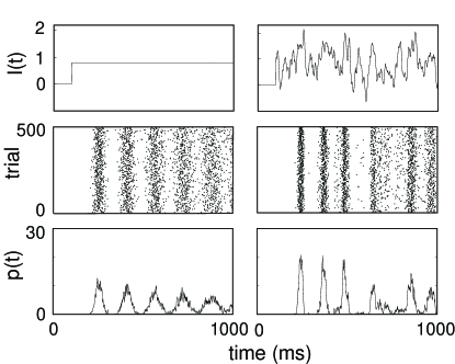
FIG. 1.: Rapidly fluctuating (panels on the right) inputs produce more reliable output spikes than a time independent stimuli (panels on the left). Panels in the top correspond to input stimulus - $I(t)$ in Eq. 1; middle ones to the 500 responses to the stimulus where the occurrence of each spike is denoted with a dot; and bottom panels depict the peri-stimulus time histogram describing the rate - $p(t)$ - at which spikes are generated in response to the stimulus $I(t)$.

By concentrating on these two extreme stimuli, these studies have somewhat obscured an issue which is central to the variability phenomenon: the relationship of the output to the timescale or timescales over which the input itself varies. The constant stimulus can be thought to have no timescale, or at best, just a timescale since onset; while in principle the noise process has indefinitely fast timescales. Thus the two extreme cases under discussion have timescales outside the range of interaction with physiological processes.

A simple dimensional argument shows that timing variability is dependent on the characteristic timescale of the input. As a consequence of noise, the neuron’s membrane potential will have fluctuations of a characteristic size (or root mean square) $\Delta V$. In order to translate this $\Delta V$ into a timing noise $\Delta t$, we have to scale the potential noise by something having units of $\Delta t/\Delta V$; the most natural such quantity at hand is the inverse of the potential’s time derivative.

While the distribution of the derivative of the potential is a reasonable measure of the degree of reliability of a particular input, one can see from a geometrical argument that the derivative of the potential at the particular time in which the potential crosses the threshold is a better estimator of stimulus reliability. The uncertainty in firing time is essentially the time during which the membrane potential is at a distance from the threshold smaller than the value of the voltage noise, and so is scaled by the derivative at this particular moment. Thus, the faster the voltage approaches the threshold (in the vecinity of the threshold), the more reliable the timing of the spike will be. The statement captures much of the phenomenology in [2, 4], and in our own data, as we will show.

FIG. 2.: Computed mean spike temporal jitter (and SEM) as a function of the estimated membrane potential’s d$V$/dt. Estimates are plotted for two noise variances: $\sigma=0.01$ ($\circ$) and $\sigma=0.02$ ($\star$). The expected inverse-law fit (with exponent $\sim 0.35$) is depicted with dotted lines. The examples in the insets illustrate two density distributions of spiking times resulting from relatively slow (inset A) or relatively fast (inset B) d$V$/dt threshold crossings. For each case, below each histograms, a few typical trajectories are also plotted showing the membrane potential preceding the threshold crossing.

We proceed now to apply this method of estimation to the situation shown in Fig. 1. A rapidly fluctuating signal was constructed [10] and the times at which spikes occurred were determined first for the deterministic condition (i.e., $\sigma=0$), and subsequently for several hundreds stochastic realizations (i.e., with identical $I(t)$ but with different stochastic realizations of the noise term in Eq. 1). At the same time the voltage derivative preceding each spike was computed over the prior fifty time steps. The fluctuating character of $I(t)$ (as illustrated in the top right panel of Fig. 1) offers the opportunity to explore a wide range of d$V$/dt at threshold crossings. To estimate the precision of spike timing we define an index of “temporal jitter” as follow: it is the absolute difference between the time at which a spike is generated in the noise-free simulation and that of the corresponding nearest spike for the stochastic realization, averaged over realizations, and over all spikes which occurr within a d$V$/dt interval of $0.1$. This quantity is plotted in Fig. 2. The data points in Fig. 2 are scattered around the expected (dotted lines) inverse relationship between the temporal jitter of the spike and the speed at which the voltage crossed the threshold. The trajectories plotted in both insets help to visualize the geometrical argument already discussed: inputs that rise more rapidly to the membrane potential threshold produce less variable spike timing.

The same basic phenomenon will affect any model of spike generation, in which the noise in the voltage-like variable is translated into jitter of its threshold crossings. To provide for a specific example, we choose a widely used model of excitable media with continuous dynamics, the FitzHugh-Nagumo model (FHN) with additive stochastic forcing [11], described by the following Langevin system:

$$\dot{V} = V-V^{3}/3-W+I(t)+\xi(t)$$ (2)

$$\dot{W} = \phi(V+a-bW)$$ (3)

The variable $V$ is the fast voltage-like variable, $W$ is the slow recovery variable; $a$, $b$ and $\phi$ are constant parameters, and $\xi(t)$ is a zero-mean Gaussian white noise of intensity $D$. According to these equations, after a spike the recovery produces an absolute refractory period during which a second spike can not occur, followed by a longer relative refractory period during which firing requires stronger perturbations.

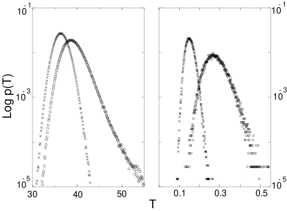
FIG. 3.: First passage time distributions for the FHN (left panel) and I-F (right panel) models, forced with constant input. In both panels, ($\times$) corresponds to high input and ($\circ$) to low.

As previously argued, it is biologically reasonable to assume that noise affects the voltage-like variable. Thus, according to our argument, a higher steady input will result in a faster approach to the threshold crossing and therefore will reduce the probability of an untimely crossing. This is confirmed in Fig. 3, where the distributions of periods are plotted for two inputs amplitudes. Note the large change in variance (1.5 to 2.34, 56$\%$) for comparably small change in the average period (36.4 to 39.1, 7$\%$) in going from high to low input, also note that the low input distribution has a supra-exponential tail. For comparison, the distribution of inter-spike intervals corresponding to the I-F model with constant input is shown. In both cases, the distribution for high input tends to a Gaussian (parabola on semi-log plot), while the low input has an exponential tail (linear on semi-log plot) as expected for Poisson-like statistics. It is interesting to notice that even though this phenomenon will affect more strongly systems with zero-frequency quiescent-to-firing bifurcations, given the longer time to integrate fluctuations at low input (i.e. the system can evolve near a homoclinic orbit), the example presented here shows that it also affects non-zero-frequency transitions like the Hopf bifurcation present in the FHN model.

III Experimental results

Thus, in neural data, one should expect to find that the output noise generically depends on the structure of the input. Experiments discussed next demonstrate the relevance of this observation for brain function. We recall that an assumption usually made in the application of information theory to neurons is that the noise introduced by the communication channel is independent of the message being transmitted, and now explore to what extent this assumption is valid in real neural data. The result is presented in Fig. 4, where different visual stimuli (i.e., the four messages) were presented to an anesthetized cat while electrophysiological recordings were made in the lateral geniculate nucleus (LGN), which is the second stage of processing in the visual pathway (see [20] for methods).

The raster plot in Panel A shows the response to a moving bar with high contrast and high speed, and Panel B shows the responses to a low contrast bar moving at low speed, both results are shown in a window of 200 msec centered at the peak of the ON response. The responses in Panel A clearly display a higher temporal precision than those for the condition in Panel B. Two further conditions were also presented, for high contrast and low speed, and for low contrast and high speed. In the inset of Fig. 4 we quantify the noise for the four messages as the “jitter” of the response onset, which we define as the average of the absolute value of the position with respect to the mean of the first spike in each trial. The messages include two conditions for the velocity and two for the contrast. For each velocity condition, the high contrast is more reliable than the low one: 8.4 msec vs. 22.1 msec, and 16.8 msec vs. 23.8 msec. Note however that the high contrast/high speed and low contrast/low speed stimuli, although they have a very similar spike response (4.17 vs. 3.86) have the largest difference in jitter (8.4 msec vs. 23.8 msec). Alternatively, we can measure the entropy difference between the corresponding first spike probability distributions (1 msec bins), which varies from 2.0 bits for low contrast/high speed vs. high contrast/high speed, to 0.6 bits for high contrast/low speed vs. high contrast/high speed. Similar results showing contrast-dependent temporal precision in LGN have been reported previously in [12], where it is also proposed that the variability is due to intrinsic noise. We also show that messages with indistinguishable mean rate responses can show large differences in their variability, in agreement with the hypothesis of the threshold crossing derivative as the relevant parameter, which can be independent of the firing rate for particular inputs.

FIG. 4.: Experimental example showing that different “messages” elicits different noise (i.e., spike temporal jitter). Results gathered from recordings in cat’s LGN where neuronal action potentials are recorded in response to the presentation of a moving bar with different contrast and speed. The inset in Panel A shows, for the conditions tested, the temporal jitter versus average number of spikes (collected during the window of 200 ms); ($\bullet$) corresponds to low contrast/high speed, (+) to high contrast/high speed, ($\bigtriangledown$) to low contrast/low speed, and ($\bigtriangleup$) to high contrast/low speed. Notice the data from moving bars of different contrast originating very different jitter. The raw data for two of the experimental conditions are presented in the raster plots of Panels A and B. Responses obtained with a moving bar of low contrast moving at low speed are plotted in Panel B. The (less variable) responses obtained with a moving bar of high contrast moving at high speed are depicted in Panel A.

IV Network architecture and reliability

The observations discussed in the previous section are restricted to the behavior of individual neurons. How can they be extended to networks of spiking elements? In principle, we can assume that input-dependent noise will be present in early stages of processing, given the relative simplicity of the neural architecture. The relevance of this phenomenon in higher order areas remains to be explored; nevertheless, we may hypothesize that unless dedicated architectures are implemented to eliminate it, significant input-dependent noise will be ubiquitous in neural processing.

Indeed, a recurring question in brain theory and computer theory is whether there are reliable ways to compute which use unreliable components. We shall now show explicitly the existence of a network topology for which the overall time reliability can be made arbitrarily better than that found in its individual neurons.

Assume a single input source $I(t)$, which “fans out” to $N$ noisy neurons $X_{i}$; these in turn “fan in”, or input into a single (also noisy) neuron $Y$. Let’s imagine an $I(t)$ constructed so that the $X_{i}$ fire once each at times $t_{i}$. If the size of the connections $X\to Y$ is set so that $Y$ fires after seeing half of the expected number of spikes coming from the $X$s, then clearly neuron $Y$ will be fire near the median time of the spike times $t_{i}$. The median, as a descriptor of the $t_{i}$, has a number of exceedingly nice properties in this context: (a) its variance decreases as $1/\sqrt{N}$, and thus the timing accuracy of $Y$ can be made better than the individual $X$s simply by choosing an appropriately large $N$; (b) the median, unlike the mean, is exceedingly robust against outliars and heavy-tailed noise; (c) the median does not require that it see the entire set $t_{i}$ but only half of it, and (d) the median is expected to lie at the time of highest concentration of the $t_{i}$, thus maximizing the timing accuracy of $Y$. This can be fully apreciated in Fig. 5. Thus, we see that different topologies will propagate spike timing accuracy in different fashions, and that one probably should expect architectural correlates in place in the brain.

To gain further insight into this issue and to study the implications of our observations on the synchronization of a neuronal network, we now concentrate on random but fixed time delays across pathways, rather than on individual timing accuracy. We modify the previous model: all neurons of the middle layer are now noise-free and in principle identical, and so are their spike trains; the neurons are integrate-and-fire units as in Eq. 1, with the further addition of a refractory period. We next model a dispersion of the transmission delay times by rigidly shifting the spike train of each individual neuron by a random value uniformly distributed between $0$ and $\delta$. The total charge that the integrating neuron receives does not depend on this shift, but when all neurons are synchronized, the derivative of the charge will be high and then we expect more reliable responses. Fig. 6 shows how the timing reliability (open circles), measured by the method of spike metrics [13], decreases with the decorrelation of the input layer. Interestingly, when the derivatives are high the response is more reliable, but by the same token, the current supplied during the refractory period will be lost. This means that smooth distributions will result in an increased effective charge and thus the rate of response of the integrating neuron is bigger when the input layer is decorrelated, as shown in Fig. 6 (open squares) .

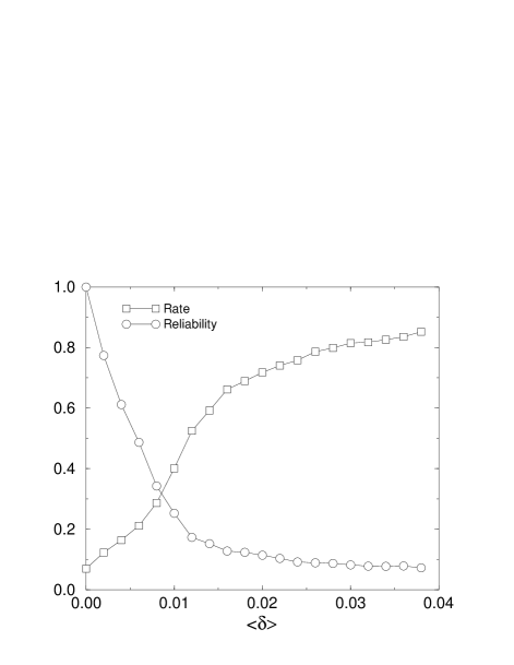
FIG. 5.: Simple model to study the effects of synchronization on the reliability of the neuronal responses. 75 Neurons synapse on a unique neuron modeled as a leaky integrate-and-fire as in Eq. 1, with the addition of a refractory period; g=0.005/s, $\sigma$=0.07, refractory period = 10 $ms$. Mean Rate and Reliability for a neuron integrating spikes over an input layer of 75 neurons. A pattern of spikes was randomly generated (3.75 Hz) and each neuron of the input layer feeds the same pattern of spikes with a delay $\delta$. The value of the other parameters are as in Fig 5. When the input layer is synchronized, $\dot{V}$ of the integrating neuron is big and the response is very reliable. In this case, part of the charge from the input layer is lost because there is no summation during the refractory period. When $\delta$ increases, the reliability decreases but the mean firing rate is increased. This suggests that a function of synchronization, which is known to occur in many different neuronal networks, might be to increase the reliability on the system at the expense of the intensity of the signal.

FIG. 6.: Reliability of a fan-out/fan-in structure. An input $I(t)$ is fanned out in parallel to $N$ identical neurons; one extra (identical) neuron fans-in: it receives input from all $N$, with the weights adjusted so as to fire once per $N/2$ input spikes. In this example, $N=51$ and $I(t)$ is a constant plus an Ornstein-Uhlenbeck process. Top panel: rasters for one instance and all 51 neurons, to illustrate the reliabilty of the middle layer. Middle panel: raster for the output neuron, 40 instances. We emphasize that the output neuron has identical parameters to the 51 neurons in the middle layer, including identical levels of internal noise. Bottom panel: a noiseless counter firing twice per $51$ spikes will implement a median measurement. Notice that both middle and bottom panels now show two spikes per each spike of the middle layer neurons, and one of them (the closest to the median) is the most reliable.

We think that this very simple concept might be of physiological relevance, in that it implies a trade-off between temporal reliability and the dynamic range of the signal: when the dynamic range is large, it is possible to afford the cost of losing part of the charge to achieve reliability, while in a situation in which the dynamic range is limited, reliability has to be sacrificed in order to preserve and propagate the signal. This suggests the possibility of integration pathways which multiplex the signal, as found in retinal adaptation.

V Conclusion

The relevance of the message-dependent nature of noise in spiking elements is, to our understanding, two-fold. One aspect is its consequences for the use of Shannon’s Information Theory as a framework to measure the information content present in the output of a neuron. This is the subject of much work recently [15]. In this regard, a basic assumption commonly made is that the noise introduced by the communication channel is independent of the message being transmitted, which allows the modeling of a neuron as a Gaussian channel [16, 17]. This is indeed desirable given that departures from the Gaussian channel have proved to be rather cumbersome; for instance, no general theory for the computation of channel capacity exists [18]. Our results render average measures of information per spike less meaningful than usually thought, and speak for the necessity of concentrating on particular individual spikes. This is specially critical when the message consists of only a few spikes (for instance, in the auditory pathway), or in the event of fast conductance modulations [19], which can dramatically affect the reliability. Thus, perhaps the most fundamental consequence of Mainen $\&$ Sejnowski’s result [3] is the implicit demonstration that cortical neurons are not always classical Gaussian channels.

A second relevant aspect is the possible anatomical correlate of this phenomenon. In this regard, we have shown that unless dedicated architecture is implemented to reduce the multiplication of noise along the processing pathways, the encoding of behaviorally relevant (not only “artificial” stimuli) can be highly degraded. Finally, we demonstrated that it is possible to design network topologies with arbitrarily large temporal reliability, and consequently one should expect an evolutionary pressure to implement them in specific areas of the brain where time accuracy is essential.

Supported in part by the Mathers Foundation (MM), NIH (JMA), Human Frontiers (LM), Rosita & Norman Winston Foundation (GAC) and Burroughs Wellcome (MS). Supercomputer resources are supported by NSF ARI Grants. Discussions with T. Gardner, S. Ribeiro and R. Crist are appreciated. We also acknowledge the valuable input from D. Reich and B. Knight.

REFERENCES

- [1] E. D. Adrian, The Basis of Sensation, Norton, New York,( 1928)
- [2] H.L. Bryant J.P. Segundo, J. Physiol. (London) 260, 279 (1976).
- [3] Z.F.Mainen T.J. Sejnowski, Science 268 (5216), 1503 (1995).
- [4] R.R. de Ruyter van Steveninck, G.D. Lewen, S.P. Strong, R. Koberle, W Bialek, Science 275 (5307), 1805 (1997).
- [5] A-K. Warzecha M. Egelhaaf, Science 283, 1927 (1999).
- [6] B.W. Knight, J. Gen. Physiol. 59, 734 (1972).
- [7] H. Risken, The Fokker-Planck Equation: Methods of Solution and Applications, Springer-Verlag, Berlin (1989).
- [8] N.G. van Kampen, Stochastic processes in physics and chemistry, Elsevier, Amsterdam (1992).
- [9] M.O. Magnasco & D. Thaler, Phys. Lett. A. 221, 287-292 (1996) .
- [10] In Fig. 1, Eq. 1 was numerically solved with parameters: , ; steady input , fluctuating input was generated as an Ornstein-Uhlenbeck process with variance 0.01 and correlation time 0.1. (for easy of presentation is plot as a ten points running average). In Fig. 3, Eq. 1 parameters are: noise variance 0.003, =0.1, high input =1.0, low =0.1; the parameters for Eq. 2-3 are: noise variance 0.003, high input , low , = 0.08, = 0.7, and = 0.8.
- [11] A. Longtin D.R. Chialvo, Phys. Rev. Lett. 81, 4012 (1998).
- [12] D.S. Reich, J.D. Victor, B.W. Knight, T. Ozaki & E. Kaplan, J. Neurophysiol. 77, 2836-2841 (1997).
- [13] J. D. Victor & K. P. Purpura, Network 8, 127-164 (1997).
- [14] C. Koch, Biophysics of computation, Oxford University Press, New York (1998).
- [15] F. Rieke, D. Warland, R. de Ruyter van Steveninck, W. Bialek, Spikes: exploring the neural code, MIT Pres, Cambridge (1997).
- [16] C. Shannon and W. Weaver, The mathematical theory of communication, University of Illinois Press, Urbana (1949).
- [17] A. Borst & F. E. Theunissen, Nat. Neurosci. 2, 947-57 (1999).
- [18] R.B. Ash, Information Theory, Dover, New York (1990).
- [19] L.J. Borg-Graham, C. Monier, Y. Fregnac, Nature 393 (6683), 369 (1998).
- [20] Experimental methods as in Martinez L.M. and Alonso J.M, Nature Neuroscience, 1,5:395-403(1998). Briefly, cats (2.5-3 kg) were anesthetized with ketamine (10 mg/kg) and thiopental sodium (20 mg/kg; maintenance 2 mg/kg/hr, IV) and paralyzed with Norcuron (0.2 mg/kg/hr, IV). Temperature (37.5o-38o C), EKG, EEG, and expired CO2 was monitored throughout the experiment. Pupils were dilated with 1 atropine sulfate and the nictitacting membranes retracted with 10 phenylephrine. A multi-electrode matrix was used for the cortical recordings. Recorded signals were collected and analyzed by a computer running Datawave Systems software (Broomfield, CO).