Multifractality in uniform hyperbolic lattices and in quasi–classical Liouville field theory

Abstract

We introduce a deterministic model defined on a two dimensional hyperbolic lattice. This model provides an example of a non random system whose multifractal behaviour has a number theoretic origin. We determine the multifractal exponents, discuss the termination of multifractality and conjecture the geometric origin of the multifractal behavior in Liouville quasi–classical field theory.

I Introduction

The concept of multifractality consists in a scale dependence of critical exponents [1]. It has been widely discussed in the literature in the context of various problems such as, for example, statistics of strange sets [2, 3, 4, 13], diffusion limited aggregation [5], wavelet transforms [6], conformal invariance [7]. This concept also proves to be useful in the context of disordered systems [25, 28]. It was recently found that the ground state wave function of two dimensional Dirac fermions in a random magnetic field has a multifractal behavior. The field theoretic investigation of the multifractality has been undertaken in the papers [8], while different interpretations of these field theoretic results from a geometrical and physical points of view were presented in [9] and [10] correspondingly. This problem was recently reanalyzed in the more general setting of systems caracterized by logarithmic correlations [25].

Our work is mainly inspired by the approach developed in [9] where the authors obtain the multifractal exponents of the critical wave function by a mapping on the problem of directed polymers on a Cayley tree. However our starting point is different and we treat a deterministic model defined on a Cayley tree. We take advantage of the fact that the Cayley tree can be isometrically embedded in a space of constant negative curvature. We assume that each vertex of the tree carries a Boltzmann weight that depends on the hyperbolic distance from a given root point. The corresponding partition function is a sum over a finite number of tree vertices and has the form of a truncated Poincaré series. Its scaling dependence on the size of the system is controlled by the probability distribution of traces of $2\times 2$ matrices which belong to a discrete subgroup of $PSL(2,{\sf I\kern-1.49994ptR})$. This distribution, obtained by using the central limit theorem for Markov multiplicative processes [30], allows us to compute the multifractal exponents and discuss the termination of multifractality. The study of the convergence of the measure on the boundary reveals some interesting links with work of Gutzwiller and Mandelbrot [13] on multifractal measures. Another interesting, although more speculative, aspect is connected with a geometric approach to Liouville field theory arising in the study of low dimensional disordered systems [8, 9, 28, 29]. We suggest that in two dimensions our model exhibits a new type of multifractal behavior which has a purely geometric origin.

This paper is organized as follows. In section II we introduce the geometrical model possessing the multifractal behavior, develop methods for its investigation and explicitly show the number theoretic origin of multifractality; section III is devoted to applications of these results to quasi–classical 2D Liouville field theory (LFT); the conclusion presents some speculations regarding the applicability of our geometric considerations to some other disordered physical systems.

II The model

We begin with the investigation of geometrical properties of lattices uniformly embedded in the hyperbolic 2-space. Lattices under consideration are defined as follows: we construct the set of all possible orbits of a given root point under the action of a discrete subgroup of $PSL(2,{\sf I\kern-1.49994ptR})$ (group of motion of the hyperbolic 2-space). We restrict ourselves with the simplest example of 3–branching Bethe lattice (Cayley tree) which is generated by reflections of zero–angled curvilinear triangle—see fig.1.

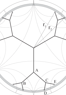
FIG. 1.: A Cayley tree in the Poincaré disc. Sample points: $A\left(-\frac{i}{2}\right)$, $\{B,C\}\left(\mp\frac{\sqrt{3}}{7}-\frac{5i}{7}\right)$, $D\left(\frac{\sqrt{3}}{8}-\frac{7i}{8}\right)$, $E\left(\frac{\sqrt{3}}{4}-\frac{3i}{4}\right)$.

The graph connecting the centers of the neighboring triangles forms a Cayley tree isometrically embedded in the Poincaré unit disc (a Riemann surface of constant negative curvature).

Consider the $n^{\rm th}$ generation of the vertices of the 3–branching Cayley tree. Denote by $r_{j}(n)$ the Euclidean distance of the vertex $j$ (which belongs to the $n^{\rm th}$ generation of the Cayley tree) from the center of the unit disc ($1\leq j\leq 3\times 2^{n-1}$). The corresponding hyperbolic (geodesic) distance $d_{j}(n)$ is given by:

$$d_{j}(n)=\ln\frac{1+r_{j}(n)}{1-r_{j}(n)}\qquad\left(r_{j}(n)=\tanh\frac{d_{j}(n)}{2}\right)$$ (1)

Define the generating function ${\cal Z}(q,N)$

$${\cal Z}(q,N)=\sum_{n=1}^{N}\left(\sum_{j=1}^{3\times 2^{n-1}}e^{-q\,d_{j}(n)}\right)$$ (2)

In a physical context ${\cal Z}(q,N)$ may be interpreted as a partition function on the hyperbolic lattice with an action linear in the length of trajectory.

The Bethe lattice involved can be constructed by the action of the discrete group $\Gamma_{\theta}$ which operates on the unit disc by a set of fractional–linear transformations. Despite the simple structure of the group it is believed that the techniques involved are quite general and could be easily generalized in order to cover more sophisticated lattices.

We are interested in the scaling dependence of the partition function ${\cal Z}(q,N)$ as a function of the size $N$ of the system. Scaling considerations suggest the following behaviour

$${\cal Z}(q,N)={\cal L}_{\rm max}^{-\tau^{\star}(q)}$$ (3)

where in our case ${\cal L}_{\rm max}=3(2^{N}-1)$ is the total number of Cayley tree vertices in the bulk restricted by the generation $n=N$.

We show below that the critical exponent $\tau(q)$ defined as follows

$$-\lim_{N\to\infty}\frac{\ln{\cal Z}(q,N)}{N}=\tau(q)$$ (4)

depends nonlinearly on $q$ i.e. exhibits the multicritical behavior (note that $\tau^{\star}=\tau/\ln 2$). Note that the free energy normalized per volume of the system $f(q,N)=-\frac{\ln{\cal Z}(q,N)}{N}$ coincides with the multifractal exponent $\tau(q)$:

$$\lim_{N\to\infty}f(q,N)=\tau(q)$$ (5)

A Numerical results

We first compute numerically the histogram, which counts the number of vertices belonging to generation $n$ (properly normalized), $W_{n}(d)$, lying in the shell $\left[d,\;d+\delta d\right]$.

In our particular computations we restrict ourselves with two cases depending on the length of the trajectories:

1. Short trajectories. We enumerate all trajectories and the computations have been carried out for all $n\in[1,N]$ up to $N=25$ generations. The figure fig.2a shows the histogram for the distribution of hyperbolic distances for $n=25$. The absolute value of number of events in the fig.2a depends on the particular choice of the width of the shell $\delta$. It can be seen from fig.2a that the corresponding plot is highly nonsymmetric with respect to the mean value $\left<d\right>$.

2. Long trajectories. For $n=200$ the enumeration of all different paths is very time consuming, therefore we compute numerically the histogram $W_{n}(d)$ developing partial ensemble of $200\,000$ directed random walks of $n=200$ step each. As $n\to\infty$ the distribution function $W_{n}(d)$ becomes more and more symmetric in accordance with the statement that there exists a central limit theorem for such random walks on noncommutative groups (see the discussion below). The results of corresponding numerical computations are presented in Fig.2b. The distribution $W_{n}(d)$ is well fitted by a Gaussian function:

   $$W_{n}(d)=A_{0}\,e^{-\frac{(d-\left<d\right>)^{2}}{2\Delta^{2}}}$$

   where for $n=200$ one has: $A_{0}\approx 1929.96$ and depends on normalization; $\left<d\right>\approx 159.18$; $\Delta^{2}\approx 17.01$.

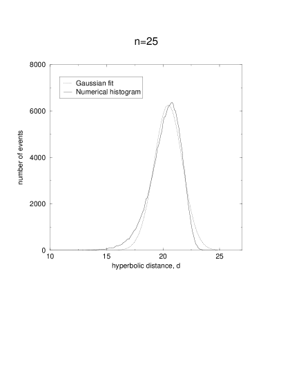
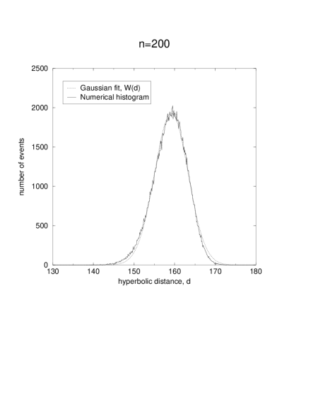
FIG. 2.: Distributions $W_{n}(d)$ up to normalization, compared to their Gaussian fits: one can notice the slow convergence from strongly nonsymetric regime for $n=25$ (a) to a Gaussian regime for $n=200$ predicted by the central limit theorem (b).

In spite of the fact that convergence to the Gaussian distribution is slow, the linear dependence in $n$ of the mean value $\left<d\right>=\gamma n$ and the variance $\left<(d-\left<d\right>)^{2}\right>\equiv\Delta^{2}=\sigma^{2}n$ is numerically evident, which permits one to get an accurate estimate of $\gamma$ and $\sigma^{2}$.

The numerical computation of the probability distribution $W_{n}(d)$ allows one to compute the multifractal exponent $\tau(q)$ following the definitions (3)–(5). The corresponding results are shown in fig.3, for $N=40$. Due to the slow convergence of the distribution, the discrepancy between numerical data (technically limited to $N\leq 40$) and the theoretical prediction can not be quantitatively taken into account. We here insist on the multifractal behaviour, shown by the non-linear depence on $q$.

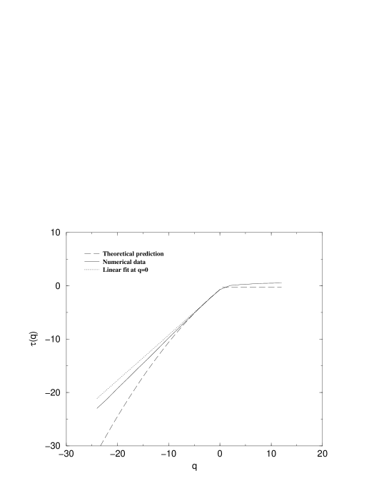
FIG. 3.: Multicritical behavior of the exponent $\tau(q)$ for $N=40$, compared to theoretical prediction.

B Analytic results

Let us return to the definition of the model and recall that the group $\Gamma_{\theta}$ acts in the hyperbolic Poincaré upper half–plane ${\cal H}^{2}=\{z\in\kern 1.00006pt{\raise 2.0236pt\hbox{$\scriptscriptstyle|$}}\kern-3.99994pt{\sf C},\,{\rm Im}(z)>0\}$ by fractional–linear transforms. The matrix representation of the generators of the group $\Gamma_{\theta}$ is well known (see, for example [23]), however for our purposes it is more convenient to take a framework that consists of the composition of standard fractional–linear transform and complex conjugacy. Namely, denoting by $\bar{z}$ the complex conjugate of $z$, we consider the following action

$$\left(\begin{array}[]{cc}a&b\\ c&d\end{array}\right):\ z\to\frac{a\bar{z}+b}{c\bar{z}+d}$$ (6)

A possible set of generators is then:

$$h_{0}=\left(\begin{array}[]{cc}1&-2/\sqrt{3}\\ 0&-1\end{array}\right),\;h_{1}=\left(\begin{array}[]{cc}1&2/\sqrt{3}\\ 0&-1\end{array}\right),\;h_{2}=\left(\begin{array}[]{cc}0&1/\sqrt{3}\\ \sqrt{3}&0\end{array}\right)$$ (7)

Choosing the point $(x_{0},iy_{0})=(0,i)$ as the tree root—see fig.4, any vertex on the tree is associated with an element $\displaystyle M_{n}=\prod_{k=1}^{n}h_{\alpha_{k}}$ where $\alpha_{k}\in\{0,1,2\}$ and is parametrized by its complex coordinates $z_{n}=M_{n}\big{(}(-1)^{n}i\big{)}$ in the hyperbolic plane.

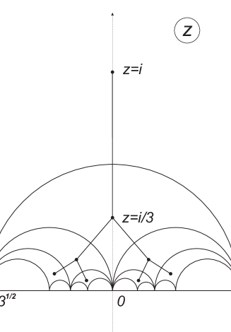
FIG. 4.: Poincaré hyperbolic upper half–plane ${\cal H}^{2}$

Strictly speaking ${\cal H}^{2}$ should be identified with $SL(2,{\sf I\kern-1.49994ptR})/SO(2)$; we here identify an element with its class of equivalence of $SO(2)$. If one denotes by $d(M_{n})\equiv d(i,z_{n})$ the hyperbolic distance between $i$ and $z_{n}$, the following identity holds

$$2\cosh\Big{(}d(M_{n})\Big{)}={\rm Tr}(M_{n}M_{n}^{{\dagger}})$$ (8)

where dagger denotes transposition.

1 Distribution function, invariant measure on the boundary and Lyapunov exponents

We are interested in the distribution function $W_{n}(d)$ which is the probability to find the tree vertices in generation $n$ at the distance $d$ from the root point. It means that we are looking for the distribution of the traces for matrices $M_{n}$ which are the irreducible products of $n$ generators. If we denote by $l(M_{n})$ the irreducible length of the word represented by the matrix $M_{n}$, then $M_{n}$ is irreducible if and only if $l(M_{n})=n$. Such word enumeration problem is simple in case of the group $\Gamma_{\theta}$, because of its free product structure: $\Gamma_{\theta}\sim{\sf Z\kern-4.49997ptZ}_{2}\otimes{\sf Z\kern-4.49997ptZ}_{2}\otimes{\sf Z\kern-4.49997ptZ}_{2}$. Indeed, if $\displaystyle M_{n}=\prod_{k=1}^{n}h_{\alpha_{k}}$ one has $l(M_{n})=n$ if and only if $h_{\alpha_{k}}\not=h_{\alpha_{k-1}}\;\forall k$. Hence we have to study the behavior of the random matrix $M_{n}$, generated by the following Markovian process

$$M_{n+1}=M_{n}h_{\alpha_{n+1}}\ {\rm with}\ \alpha_{n+1}=\left\{\begin{array}[]{ll}(\alpha_{n}+1)\,{\rm mod}\,3&\ \mbox{with probability $\frac{1}{2}$}\vskip 6.0pt plus 2.0pt minus 2.0pt\\ (\alpha_{n}+2)\,{\rm mod}\,3&\ \mbox{with probability $\frac{1}{2}$}\end{array}\right.$$ (9)

We use the standard methods of random matrices and consider the entries of the $2\times 2$–matrix $M_{n}$ as a 4–vector ${\cal V}_{n}$. The transformation $M_{n+1}=M_{n}h_{\alpha}$ reads

$${\cal V}_{n+1}=\left(\begin{array}[]{ll}h_{\alpha}^{{\dagger}}&0\\ 0&h_{\alpha}^{{\dagger}}\end{array}\right)\;{\cal V}_{n}$$ (10)

This block–diagonal form allows one to restrict ourselves to the study of one of two 2–vectors, composing ${\cal V}_{n}$, say $v_{n}$. Parametrizing $v_{n}=(\varrho_{n}\cos\theta_{n},\varrho_{n}\sin\theta_{n})$ and using the relation $d(M_{n})\equiv d_{n}\simeq 2\ln\varrho_{n}$ valid for $n\gg 1$, one gets a recursion relation $v_{n+1}=h_{\alpha}^{{\dagger}}v_{n}$ in terms of hyperbolic distance $d_{n}$:

$$d_{n+1}=d_{n}+\ln\,\left[\frac{5}{3}+\frac{4}{3}\cos(2\theta_{n}+\varphi_{\alpha})\right]$$ (11)

where $\varphi_{\alpha}$ depends on the transform $h_{\alpha}$ through $\displaystyle\varphi_{\alpha}=(2\alpha-1)\pi/3\;(\alpha=0,1,2)$, while for the angles one gets straightforwardly

$$\tan\theta_{n+1}=h_{\tilde{\alpha}}\Big{(}\tan(\theta_{n})\Big{)}$$ (12)

and the change $\alpha\rightarrow\tilde{\alpha}$ means the substitution $(0,1,2)\rightarrow(1,0,2)$. Action of $h_{\alpha}$ is still fractional–linear.

Define now three invariant measures $\mu_{\alpha}(\theta)$ corresponding to transformations of $M_{n}$ ($n\gg 1$) whose last step is given by a matrix $h_{\alpha}$. The form of (12) suggests to consider the corresponding $\mu_{\alpha}(x)$ with $x=\tan\theta$. We are then led to study the action of $\Gamma_{\theta}$ restricted on the real line parametrized by $x$. Interesting properties of the average $\overline{\mu}=(\mu_{0}+\mu_{1}+\mu_{2})/3$ have been discussed by Gutzwiller and Mandelbrot [13]. In particular they pointed out the connexion with the arithmetic function $\beta(\xi)$ which maps some number $\xi\in[0,1]$ written as a continued fraction expansion

$$\frac{1}{n_{1}+\displaystyle\frac{1}{n_{2}+\ldots}}$$

to the real number $\beta$ whose binary expansion is made by the sequence of $n_{1}-1$ times 0, followed by $n_{2}$ times 1, then $n_{3}$ times 0, and so on. To account for this fact, one has first to notice that the construction (9) of any word $M$ in $\Gamma_{\theta}$ is exactly encoded by the binary representation of a real $\xi$, the $n$’s letter of this expansion being $\alpha_{n+1}-\alpha_{n}+1\,{\rm mod}\,3$. The second argument, due to Series [14], is that the real part of the vertex $M(i)$ is precisely the continued fraction $\mu(\xi)$. Therefore $\beta(\xi)$ has to be proportional to the “number” of vertices lying in the interval $[0,\xi]$, that is to $\overline{\mu}([0,\xi])$. Taking the limit $n\rightarrow\infty$ is not well defined. An alternative, which was used in this work, is to define $\mu_{\alpha}(x)$ as the limit of the following recurrency:

$$\mu_{\alpha}^{(n+1)}(x)=\frac{1}{2}\left|\frac{dh_{\alpha}(x)}{dx}\right|\sum_{\alpha^{\prime}\not=\alpha}\mu_{\alpha^{\prime}}^{(n)}\Big{(}h_{\alpha^{\prime}}(x)\Big{)}$$ (13)

The symetry of such expression leads, after summing over ${\alpha}$, to the following relation admitting as fixed point $\overline{\mu}(x)$ at $n\to\infty$:

$$\mu^{(n+1)}(x)=\frac{1}{3}\sum_{\alpha=0}^{2}\mu^{(n)}\Big{(}h_{\alpha}(x)\Big{)}\left|\frac{dh_{\alpha}(x)}{dx}\right|$$ (14)

FIG. 5.: Invariant measure $\overline{\mu}$ as a function of $\theta$

The convergence $\mu^{(n)}(x)\to\overline{\mu}(x)$ for $n\to\infty$ is assured by ergodic properties of such functional transform in case of equation (14), and has been successfully checked numerically by comparing to direct sampling of different orbits. Obtaining $\mu_{\alpha}$ for $\alpha=\{0,1,2\}$ from $\overline{\mu}$ is not difficult, taking into account the symmetric role that they play with respect to the three intervals $I_{0}=]-\infty,-1/\sqrt{3}],\ I_{2}=[-1/\sqrt{3},1/\sqrt{3}],\ I_{1}=[1/\sqrt{3},+\infty[$ (see fig.5). Contracting properties of $h_{\alpha}(x)$ allow convergence of (14) only if

$$\mu_{k}(x)=3\chi_{I_{k}}(x)\overline{\mu}(x)$$ (15)

where $\chi_{I_{k}}$ is the characteristic function of the interval $I_{k}$.

We would like to point out an interesting fact, even if far from being rigorous, which is very similar to the argument put forward in [13] for justifying the connexion between the invariant measure and the arithmetic function $\beta(\xi)$. It has been shown in [22] that the lattice under consideration can be isometrically embedded in a 2–manifold ${\cal M}=\{c|\eta(z)|^{4},\,z\in{\cal H}^{2}\}$, where

$$\eta(z)=e^{\pi iz/12}\prod_{n=1}^{\infty}(1-e^{2\pi inz})$$

is the Dedekind $\eta$–function. The mountain range (relief) ${\cal M}$ displays a very steep valley structure, and our tree lattice was defined as the ridges of this relief. The natural “counting” of vertices whose real part lies in $[0,\xi]$ in [13] is in our case equivalent to counting the number of maxima of $|\eta(x+i0^{+})|^{4}$, that can be directly reexpressed as a density if one admits that all maxima are equivalent and well separated:

$$\overline{\mu}(x)\sim\frac{|\eta(x+i0^{+})|^{4}}{\int_{0}^{1}|\eta(t+i0^{+})|^{4}dt}$$ (16)

The intriguing fact is that $\eta^{4}$ is an automorphic form of weight 2, what makes $|\eta|^{4}$ precisely a possible fixed point of Eq.(14). We recall the fundamental property of automorphic forms $f$ of weight 2 under the action of $SL(2,{\sf I\kern-1.49994ptR})$:

$$f(z)=\frac{e^{i\phi(a,b,c,d)}}{(cz+d)^{2}}f\left(\frac{az+b}{cz+d}\right)$$ (17)

The main problem is that the boundary behavior of automorphic forms is far from trivial (see [27]), and (16) has no rigorous mathematical sense. In particular compatibility of (14) and (16) is not obvious even numerically. Nevertheless we insist on the fact that $\mu_{k}$ is defined with no ambiguity by (14), what enables us to compute the desired $W_{n}(d)$. The crucial point here, already required for convergence of $\mu^{(n)}$, is ergodicity property of $\theta_{n}$. It means that for $n\gg 1$, the distribution of $\theta_{n}$ is exactly given by $\overline{\mu}(\theta)$, independently of $n$ and initial condition. Then, denoting by $d_{n}^{\alpha}$ the value $d_{n}$ obtained for a word ending with $h_{\alpha}$, one can transform (11) in the following way:

$$d_{n+1}=\frac{1}{3}\sum_{\alpha=0}^{2}\left(d_{n}^{\alpha}+\ln\left[\frac{5}{3}+\frac{4}{3}\cos(2\theta_{n}+\varphi_{l})\right]\right)$$ (18)

with the condition $l\not=\alpha$. Thus we obtain

$$\left<e^{ikd_{n}}\right>=\frac{1}{6}\sum_{k=0}^{2}\sum_{j\not=k}\left[\int_{-\pi/2}^{\pi/2}d\theta\mu_{k}(\theta)\left(\frac{5}{3}+\frac{4}{3}\cos(2\theta+\varphi_{j})\right)^{ik}\right]^{n}$$ (19)

which finally leads to

$$W_{n}(d)=\frac{1}{2\pi}\int_{-\infty}^{\infty}dk\,e^{-ikd}\left[\int_{0}^{\frac{\pi}{3}}d\theta\mu_{1}(\theta-\frac{\pi}{6})\left(\frac{5}{3}+\frac{4}{3}\cos 2\theta\right)^{ik}\right]^{n}$$ (20)

This form suggests that for $n$ large $W_{n}(d)$ satisfies a central limit theorem. Indeed such a theorem exists (see [24, 30]) for Markovian processes, provided that the phase space is ergodic. We are then led to compute only the first two moments (Lyapunov exponents) which gives

$$\gamma=\frac{\left<d\right>}{n}=\int_{0}^{\frac{\pi}{3}}d\theta\mu_{1}(\theta-\frac{\pi}{6})\ln\left(\frac{5}{3}+\frac{4}{3}\cos 2\theta\right)\approx 0.792$$ (21)

and

$$\sigma^{2}=\frac{\left<(d-\left<d\right>)^{2}\right>}{n}=\gamma_{2}-\gamma^{2}$$ (22)

with

$$\gamma_{2}=\int_{0}^{\frac{\pi}{3}}d\theta\mu_{1}(\theta-\frac{\pi}{6})\ln^{2}\left(\frac{5}{3}+\frac{4}{3}\cos 2\theta\right)\approx 0.68$$ (23)

Numerical simulations presented in previous section yield $\gamma\approx 0.793$ and $\gamma_{2}\approx 0.66$, which finally allow us to conclude that for $n\gg 1$ $W_{n}(d)$ has a Gaussian behavior

$$W_{n}(d)=A\,e^{-\frac{(d-n\gamma)^{2}}{2\sigma^{2}n}}$$ (24)

centered at $\gamma n$ and of variance $\sigma^{2}n$ ($A$ is the normalization).

The numerical values of the Lyapunov exponents $\gamma$ and $\gamma_{2}$ (see Eqs.(21) and (23)) are obtained by means of semi–numerical procedure which involves the numerical information about the invariant measure $\mu_{1}(\theta)$. However one can get the estimates for the Lyapunov exponents $\gamma$ and $\gamma_{2}$ by approximating the measure $\mu_{1}(\theta)$ on the interval $0\leq\theta\leq\frac{\pi}{3}$ in two different ways:

$$\begin{array}[]{l}\displaystyle\mu_{1}(\theta-\frac{\pi}{6})\approx\mu_{1}^{A}(\theta)=\frac{3}{\pi}\vskip 6.0pt plus 2.0pt minus 2.0pt\\ \displaystyle\mu_{1}(\theta-\frac{\pi}{6})\approx\mu_{1}^{B}(\theta)=\frac{3}{2}\sin(3\theta)\end{array}$$ (25)

Both measures $\mu_{1}^{A}$ and $\mu_{1}^{B}$ are properly normalized on the interval $[0,\frac{\pi}{3}]$. Substituting (25) in (21) and (23) and computing (analytically for $\gamma$) the corresponding integrals, one finally gets:

$$\mu_{1}^{A}:\ \left\{\begin{array}[]{l}\gamma\approx 0.749\\ \gamma_{2}\approx 0.665\end{array}\right.\qquad\mu_{1}^{B}:\ \left\{\begin{array}[]{l}\gamma\approx 0.792\\ \gamma_{2}\approx 0.684\end{array}\right.$$ (26)

As one can see, the agreement between numerical values of Lyapunov exponents obtained for the measures $\mu_{1}$ and its approximants $\mu_{1}^{A,B}$ is reasonable for $\mu_{1}^{A}$ and very good for $\mu_{1}^{B}$.

2 Multifractal exponents

The partition function ${\cal Z}(q,N)$ introduced in (2) can be defined for any discrete subgroup of $PSL(2,{\sf I\kern-1.49994ptR})$ of generic element $\tau$ by

$${\cal Z}(q,N)=\sum_{\tau,\,l(\tau)\leq N}e^{-qd(\tau)}$$ (27)

and the associated critical exponent is then

$$\tau(q)=-\lim_{N\to\infty}\frac{\ln{\cal Z}(q,N)}{N}$$ (28)

The probability distribution (24) enables us to rewrite (27) for the group $\Gamma_{\theta}$ in the limit $n\gg 1$ as follows

$${\cal Z}(q,N)=\sum_{n=1}^{N}3\times 2^{n-1}a_{n}$$ (29)

where

$$a_{n}=\int_{0}^{\infty}e^{-qt}W_{n}(t)dt=\int_{0}^{\infty}A\,e^{-\frac{(t-n\gamma)^{2}}{2n\sigma^{2}}}e^{-qt}dt$$ (30)

The following two cases should be distinguished:

• For $q<\gamma/\sigma^{2}$, the minimum of the exponent in Eq.(30) is within the range of integration and

  $$a_{n}\sim e^{-n\gamma q+n\sigma^{2}q^{2}/2}$$ (31)

  hence

  $${\cal Z}(q,N)\sim\frac{3}{2}\sum_{k=1}^{N}e^{k(\ln 2-\gamma q+\sigma^{2}q^{2}/2)}$$ (32)

  The convergence of the sum (32) for $N\to\infty$ depends on the sign of the function in the exponent. For

  $$q<q_{0}=\frac{\gamma-\sqrt{\gamma^{2}-2\sigma^{2}\ln 2}}{\sigma^{2}}$$ (33)

  one has $-\ln 2+\gamma q-\sigma^{2}q^{2}/2>0$ and the multifractal exponent is

  $$\tau(q)=-\ln 2+\gamma q-\sigma^{2}q^{2}/2$$ (34)

  while for $q>q_{0}$, the series ${\cal Z}(q,N)$ converges and $\tau(q)=0$ what signals the termination of the multifractality. Note that $q_{0}$ is real at least in the case of the group $\Gamma_{\theta}$.

• For $q>\gamma/\sigma^{2}$ the minimum of the exponent in Eq.(30) is out of the range of integration and

  $$\ln a_{n}\sim-\frac{n\gamma^{2}}{2\sigma^{2}}$$ (35)

  hence ${\cal Z}(q,N)$ is no longer extensive in $N$, which leads to $\tau(q)=\tau(q_{0})=0$.

The nonlinear dependence on $q$ obtained above shows the multifractal behaviour of this model below the termination point $q_{0}$. It seems more transparent to summarize all these results in a table

$q<\gamma/\sigma^{2}$	$q<q_{0}=\frac{\gamma-\sqrt{\gamma^{2}-2\sigma^{2}\ln 2}}{\sigma^{2}}$ $\qquad\tau(q)=-\ln 2+\gamma q-\sigma^{2}q^{2}/2$ $q>q_{0}=\frac{\gamma-\sqrt{\gamma^{2}-2\sigma^{2}\ln 2}}{\sigma^{2}}$ $\qquad\tau(q)=0$
$q>\gamma/\sigma^{2}$	$\tau(q)=\tau(q_{0})=0$

3 Conformal mapping approach to computation of partition function and multifractal exponent

We propose in this section a completely different approach allowing to get a closed analytic expression for the partition function similar to ${\cal Z}(q,N_{\rm max})$ (see Eq.(2)). The construction presented below is a by-product of our former investigations of analytic structure of the covering Riemann space of the multi–punctured complex plane (see, for review [21]). We explore the properties of the Jacobian of conformal mapping of the infinite complex plane with a triangular lattice of punctures into the unit disc parametrized by $w=re^{i\alpha}$, which in this particular case represents the multi–sheeted universal covering space [21]. Namely, we define two functions $f(r,\alpha)$ and $g(r)$:

$$f(r,\alpha)=c\frac{\left|\theta_{1}^{\prime}\left(0,e^{i\pi\zeta(w)}\right)\right|^{8/3}}{|1+iw|^{4}}\equiv c\frac{\left|\eta(\zeta(w))\right|^{8}}{|1+iw|^{4}},\quad g(r)=\frac{1}{(1-r^{2})^{2}}$$ (36)

where

$$\left\{\begin{array}[]{l}\displaystyle\theta_{1}^{\prime}\left(0,e^{i\pi\zeta}\right)=2\,e^{i\frac{\pi}{4}\zeta}\sum_{n=0}^{\infty}(-1)^{n}(2n+1)\,e^{i\pi n(n+1)\zeta}\vskip 6.0pt plus 2.0pt minus 2.0pt\\ \displaystyle\zeta(w)=e^{-i\pi/3}\,\frac{w+e^{i\pi/6}}{w-i}\vskip 6.0pt plus 2.0pt minus 2.0pt\\ \displaystyle c=\left|\theta_{1}^{\prime}\left(0,e^{i\pi\zeta(0)}\right)\right|^{-8/3}\approx 0.933293\end{array}\right.$$ (37)

One can show that the functional equation

$$\frac{f(r,\alpha)}{g(r)}-1=0$$ (38)

has a family of solutions $(r_{\rm c},\alpha_{\rm c})$ exactly at positions of 3–branching Cayley tree isometrically embedded in the hyperbolic unit disc (in the Klein’s model of the surface of constant negative curvature). In fig.6 we have plotted the 3D section of the function

$$u(r,\alpha)=\frac{f(r,\alpha)}{g(r)}$$ (39)

in polar coordinates $(r,\alpha)$ for $0.9<u(r,\alpha)\leq 1$. The function $u(r,\alpha)$ has local maxima with one and the same value $u=1$ only at the coordinates of isometric embedding of 3–branching Cayley tree in the hyperbolic unit disc. The proof of this fact is given in Appendix A.

Thus, we can rewrite (2) in the following closed form (recall that Euclidean distance $r$ and the corresponding hyperbolic distance $d$ are linked by the relation (1))

$$\tilde{{\cal Z}}(q,d)=\frac{1}{2\pi}\int\limits_{0}^{r(d)}\int\limits_{0}^{2\pi}\;e^{-q\ln\frac{1+r}{1-r}}\delta\left(\ln u(r,\alpha)\right)\left|\frac{d\ln u(r,\alpha)}{dr}\right|rdrd\alpha$$ (40)

where for $\delta[\ln u(x)]$ we use the standard integral representation $\delta[\ln u(x)]=\frac{1}{2\pi}\int\limits_{-\infty}^{\infty}d\xi\,[u(x)]^{i\xi}$.

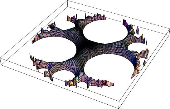
FIG. 6.: 3D parametric plot of the function $u(r,\alpha)$ in the section $0.9<u(r,\alpha)\leq 1$.

It is noteworthy to pay attention to the difference between the partition functions ${\cal Z}(q,N)$ (Eq.(2)) and $\tilde{{\cal Z}}(q,d)$ (Eqs.(27) and (40)). The function ${\cal Z}(q,N)$ counts the weighted number of Cayley tree vertices up to the generation $N$ for nonfixed maximal radius $r(d)=\tanh(d/2)$ in the hyperbolic unit disc, while the function $\tilde{{\cal Z}}(q,d)$ counts the weighted number of Cayley tree vertices within the hyperbolic disc of radius $r(d)$ for nonfixed maximal generation $N$. The last partition function is in fact related to the number of tree vertices inside the disc of radius $d$. This is the content of the famous circle problem first formulated by Gauss for the Euclidean lattice ${\sf Z\kern-4.49997ptZ}^{2}$. The extension to the non-Euclidean case is due to Delsarte [31] (see also [18]).

III Multifractality in 2D quasi–classical Liouville field theory

Our starting point is the family of normalized wave functions $\psi_{k}({\bf x})$ defined as follows

$$\psi_{k}({\bf x})=\frac{|{\bf x}|^{k}e^{-\varphi({\bf x})}}{\left[\int d{\bf x}\,|{\bf x}|^{2k}e^{-2\varphi({\bf x})}\right]^{1/2}}$$ (41)

where integration extends to a disc of radius $R$ and the potential $\varphi({\bf x})$ is distributed with Gaussian distribution function

$$P[\varphi({\bf x})]\propto\exp\left\{-\frac{1}{2g}\int d{\bf x}\left(\nabla\varphi({\bf x})\right)^{2}\right\}$$ (42)

The problem defined in (41)–(42) appears in various models which will be discussed in the next section.

The multifractal exponent for the quenched and annealed distributions of disorder in (41)–(42) can be computed in the standard way

$$\begin{array}[]{ll}\displaystyle\tau_{\rm qu}(q)=-\lim_{R\to\infty}\frac{\left<\ln Q(q,R)\right>}{\ln R}&\mbox{for quenched disorder}\vskip 6.0pt plus 2.0pt minus 2.0pt\\ \displaystyle\tau_{\rm an}(q)=-\lim_{R\to\infty}\frac{\ln\left<Q(q,R)\right>}{\ln R}&\mbox{for annealed disorder}\end{array}$$ (43)

where $Q(q,R)=\int d{\bf x}|\psi_{k}({\bf x})|^{2q}$ and the brackets $\left<...\right>$ denote averaging with the distribution $P[\varphi({\bf x})]$.

We pay attention to the case of annealed disorder and our aim is to evaluate the correlation function

$$\left<Q(q,R)\right>=\int d{\bf x}\left<|\psi_{k}({\bf x})|^{2q}\right>$$ (44)

The averaging $\left<...\right>$ in (44) means

$$\left<...\right>_{S[\varphi]}=\int{\cal D}[\varphi({\bf x})]e^{-S[\varphi({\bf x})]}$$ (45)

where

$$S[\varphi({\bf x})]=\frac{1}{2g}\int d{\bf x}\left\{\left(\nabla\varphi({\bf x})\right)^{2}\right\}$$ (46)

In order to take into account proper normalization of the wave function $\psi_{k}({\bf x})$ it is convenient to use a Lagrange multiplier $\lambda$, so that eventually

$$\left<Q(q,R)\right>=\int d{\bf x}_{0}\int{\cal D}[\varphi({\bf x})]e^{-2q\left(\varphi({\bf x}_{0})-k\ln|{\bf x}_{0}|\right)}\,e^{-S_{k}[\varphi({\bf x})]}$$ (47)

where

$$S_{k}[\varphi({\bf x})]=\frac{1}{2g}\int d{\bf x}\left\{\left(\nabla\varphi({\bf x})\right)^{2}+2\lambda g\left(|{\bf x}|^{2k}e^{-2\varphi({\bf x})}-\frac{1}{\pi R^{2}}\right)\right\}$$ (48)

is the action of 2D Liouville Field Theory (LFT).

The careful treatment of the quantum LFT in the case $k=0$ (see for review [15]) enables one to find the conformal weights $\Delta\left(e^{-2q\varphi}\right)=q({\cal Q}-q)$, where ${\cal Q}(g)$ is the “background charge”, obtained by imposing conformal invariance of $S_{0}[\varphi]$. The authors of work [8] have related the value $\Delta\left(e^{-2q\varphi}\right)$ to the critical exponent $\tau_{\rm an}(q)$ in the scaling dependence of the average inverse participation ratio (44)

$$\left<Q(q,R)\right>\sim R^{-\tau_{\rm an}(q)}$$ (49)

Despite the multiscaling exponent $\tau_{\rm an}(q)$ has been computed in the general framework of Conformal Field Theory (CFT) few years ago, from our point of view, the geometrical interpretation of the multifractal behavior in the model has not yet been cleared up. A more physical approach put forward in [9] exploits an analogy between this model and the problem of directed polymers on a Cayley tree. This analogy is supported by the fact that in both cases the correlation functions grow logarithmically with the distance. For directed polymers it is the correlation function of the random potential defined on the tree vertices that scales logarithmically with the ultrametric distance (i.e. distance along the tree). The same logarithmic behaviour occurs in $2D$ Gaussian Field Theory [8].

We adopt a different point of view. Let us notice that the tree structure (conjectured by C.Chamon et al) emerges quite naturally from the Liouville field theory treated at a semi-classical level. Our idea is as follows. Indeed there is not just one saddle point solution but a whole orbit of solutions parametrized by $SL(2,{\sf I\kern-1.49994ptR})$. If one further assumes that the integration has to be performed not over the whole group but only over a subgroup (for instance $\Gamma_{\theta}$), one recovers quite naturally the model defined in section II.

Our starting point is the semi–classical ($g\rightarrow 0$) treatment of (47) (a similar approach can be found in [19]). Using a saddle point method, one is led to the classical equation

$$\Delta\varphi-2qg\delta^{2}({\bf x}-{\bf x}_{0})+2\lambda g|{\bf x}|^{2k}\;e^{-2\varphi}=0$$ (50)

which gives, after integration

$$\lambda=q-F/2g$$ (51)

where

$$F=\int d{\bf x}\Delta\varphi$$

is the magnetic flux. We then introduce the shifted field

$$\tilde{\varphi}({\bf x})=\varphi({\bf x})-\ln|{\bf x}|^{k}$$ (52)

and taking into account that

$$\Delta\tilde{\varphi}({\bf x})=\Delta\varphi({\bf x})-2\pi k\delta^{2}({\bf x})$$ (53)

we end up with the following equation

$$\Delta\tilde{\varphi}+2\pi k\delta^{2}({\bf x})-2q\,g\delta^{2}({\bf x}-{\bf x}_{0})+(2q\,g-F)e^{-2\tilde{\varphi}}=0$$ (54)

The most general solution of (54) (away from singularities) in Euclidean space of complex coordinate $z$ can be written as follows [15]

$$e^{-2\tilde{\varphi}}=\frac{4}{|F-2qg|}\;\frac{\partial_{z}A(z)\partial_{\overline{z}}B(\overline{z})}{\Big{(}1+\epsilon A(z)B(\overline{z})\Big{)}^{2}}$$ (55)

where $A(z)$ and $B(\overline{z})$ are correspondingly holomorphic and anti–holomorphic functions of $z$ and $\epsilon={\rm sign}(F-2q\,g)$. The semi–classical treatment assumes $g$ to be small, hence in order to have real $\tilde{\varphi}$ in Eq.(55) we should put $\epsilon=1$, i.e. $q\ll F/2g$. The relevant solution of (55), compatible with the singularities, reads

$$e^{-2\tilde{\varphi}_{cl}(z)}=\frac{4(k+1)^{2}}{F}\frac{(z\bar{z})^{k}}{\left(1+(z\bar{z})^{k+1}\right)^{2}}$$ (56)

The normalization condition of the wave function is then satisfied only if $F=4\pi(k+1)$. We would like to stress that for $k=0$ we here recover the critical value $4\pi$ of the magnetic flux: uniqueness of the ground state wave function holds only below this value. It also should be mentioned that our analysis does not depend on a peculiar basis of eigenfunctions and the results presented here can be extended to wave functions of the form $\psi(z)=P_{k}(z)e^{-\varphi(z)}$, $P_{k}$ being a polynomial of degree $k$. It is noteworthy that (56) is an algebraically decaying wave function, what is, following [8], a signature of the existence of prelocalized states.

Using the fact that the Liouville field is not exactly a scalar but varies under holomorphic coordinate transformations $z\rightarrow w(z)$ as

$$\tilde{\varphi}(z)\to\tilde{\varphi}\left(w(z)\right)-\ln|w^{\prime}(z)|,$$ (57)

one can check that the set of solutions (56) is invariant under the following family of transformations, parametrized by the group $PSL(2,\kern 1.00006pt{\raise 2.0236pt\hbox{$\scriptscriptstyle|$}}\kern-3.99994pt{\sf C})$:

$$z\to w_{k}(z;a,b,c,d)=\left(\frac{az^{k+1}+b}{cz^{k+1}+d}\right)^{\frac{1}{k+1}}$$ (58)

The orbit of $\tilde{\varphi}_{cl}(z)$ is then given by

$$\tilde{\varphi}_{cl}\left(z;a,b,c,d\right)=\frac{1}{2}\ln\left(\frac{\pi\left(|az^{k+1}+b|^{2}+|cz^{k+1}+d|^{2}\right)^{2}}{(z\bar{z})^{k}}\right)$$ (59)

Up to redefinition of the measure $d\tau$ on $PSL(2,\kern 1.00006pt{\raise 2.0236pt\hbox{$\scriptscriptstyle|$}}\kern-3.99994pt{\sf C})$, we restrict the domain of integration to $PSL(2,{\sf I\kern-1.49994ptR})$.

Due to the angular symmetry of (56), we take points of the form $z=i^{\frac{1}{k+1}}\rho$ ($\rho\in{\sf I\kern-1.49994ptR}$), and following [19] we rewrite (44)–(46)

$$\left<\rho^{2qk}e^{-2q\varphi(\rho)}\right>_{S_{k}[\varphi]}=R^{-\frac{4\pi(k+1)^{2}}{g}}{\rm Det}\left[\frac{\delta^{2}S_{k}}{\delta\varphi^{2}}\right]^{-1/2}\int_{PSL(2,{\sf I\kern-1.04996ptR})}e^{-2q\tilde{\varphi}_{cl}(\rho,\tau)}d\tau$$ (60)

Let us denote

$$\tau=\left(\begin{array}[]{cc}a&b\\ c&d\end{array}\right)\quad{\rm and}\quad\nu_{\rho}=\left(\begin{array}[]{ll}\rho^{(k+1)/2}&0\\ 0&\rho^{-(k+1)/2}\end{array}\right)$$ (61)

then we can rewrite (60) as follows

$$\left<\rho^{2qk}e^{-2q\varphi(\rho)}\right>_{S_{k}[\varphi]}\propto\rho^{-2q}\int_{PSL(2,{\sf I\kern-1.04996ptR})}e^{-2q\ln{\rm Tr}\left[(\tau\nu_{\rho})(\tau\nu_{\rho})^{{\dagger}}\right]}d\tau=\rho^{-2q}I(\rho,q)$$ (62)

where we have got rid of irrelevant factors and the function $I(\rho,q)$ reads

$$I(\rho,q)=\int_{PSL(2,{\sf I\kern-1.04996ptR})}\left[2\cosh d(i,\tau\nu_{\rho}(i))\right]^{-2q}d\tau$$ (63)

Instead of summing over the whole group $PSL(2,{\sf I\kern-1.49994ptR})$, we restrict the sum over a discrete subgroup, $\Gamma_{\theta}$ in our case. Even if this discretization of the saddle manifold has no evident physical justification, we believe that the model obtained yields interesting results. It leads to consider the so-called Poincaré series (see [26] for review) $H$, defined as follows

$$I(\rho,q)=H(i,\nu_{\rho}(i),q)=\sum_{\tau\in\Gamma_{\theta}}\left[2\cosh d(i,\tau\nu_{\rho}(i))\right]^{-2q}$$ (64)

As shown in [26], the series $H$ does not converge for $q<q^{\star}$ with $q^{\star}$ depending on $\Gamma_{\theta}$ only (the analysis of the previous sections show that we roughly may set $q^{\star}\simeq q_{0}/2$). A new dependence on $\rho$ occurs only if $H$ does not converge, we will therefore consider only this regime. We must introduce in this case a cut-off ${\cal N}$ to regularize the series, and finally study asymptotics of the finite sum

$$I_{{\cal N}}(\rho,q)=H_{{\cal N}}(i,\nu_{\rho}(i),q)=\sum_{\tau\in\Gamma_{\theta}/l(\tau)\leq{\cal N}}\left[2\cosh d(i,\tau\nu_{\rho}(i))\right]^{-2q}$$ (65)

This Poincaré series has the same asymptotic properties as the one that defines our model. In particular it will exhibit a multifractal behaviour in ${\cal N}$. However what really matters for a physical system is the multifractal behaviour under transformations parametrized by $\rho$. We therefore have to relate the behaviour in the group manifold to the behaviour in the real space. This will be achieved through a renormalization transformation of the form

$$I_{{\cal N}}(\rho,q)=C\rho^{\kappa}I_{{\cal N}^{\prime}({\cal N},\rho)}(1,q)$$ (66)

Appendix B provides a heuristic derivation which gives

$$I_{{\cal N}}(\rho,q)=C\rho^{-(k+1)\ln 2/\gamma}I_{{\cal N}+\frac{(k+1)}{\gamma}\ln\rho}(1,q)$$ (67)

Comparing (27) and (64) gives $I_{{\cal N}}(1,q)\approx{\cal Z}(2q,{\cal N})$. Therefore

$$I_{{\cal N}}(\rho,q)=C\rho^{-(k+1)\ln 2/\gamma}{\cal Z}(2q,{\cal N}+\frac{k+1}{\gamma}\ln\rho)$$ (68)

This relation allows to extract the scale dependence in $\rho$ for a given cut-off ${\cal N}$. Using the asymptotics of ${\cal Z}$ obtained in previous sections yields

$$\left<\rho^{2qk}e^{-2q\varphi(\rho)}\right>_{S_{k}[\varphi]}\propto\rho^{-2q-(k+1)\ln 2/\gamma}\,\rho^{-\frac{k+1}{\gamma}\tau(2q)}$$ (69)

with the notations of previous sections. After integrating over the whole domain we arrive at the final expression for the multifractal exponent ${\tau}_{\rm an}(q)$:

$$\tau_{\rm an}(q)=-\lim_{R\to\infty}\frac{\ln\left<Q(q,R)\right>}{\ln R}=\displaystyle 2(q-1)\left(1-\frac{(k+1)\sigma^{2}}{\gamma}\,q\right)\ \mbox{for $q<q_{0}/2$}$$ (70)

with $q_{0}$ defined in (33). The regular term $2(q-1)$ corresponds to the one obtained in [9] for $g\to 0$. Multifractality of the wave function is induced by the quadratic term, which is directly related to geometric properties of the saddle point hyperbolic manifold (target space), and holds in absence of any random potential in this target space. The regime $q>q_{0}/2$ is not affected by these geometric properties.

IV Conclusion

The wave function $\psi_{k}({\bf x})$ introduced in (41) belongs to the general class of exponential functionals of free fields. Such functionals appear in several physical contexts.

1. The square of the wave function (for $k=0$) may be interpreted as the equilibrium Gibbs measure in the random potential $\varphi({\bf x})$. In the 1D case the problem was first studied in [32]. A rather deep and complete analysis of this problem was recently presented in [25].

2. Exponential functionals of free fields play an important role in the context of one dimensional classical diffusion in a random environment. Their probability distribution controls the anomalous diffusive behaviour of particles at large time [33]. They also arise in the study of disordered samples of finite length [34, 29]. Some mathematical properties are discussed in [35].

3. In the context of one dimensional localization in a random potential such functionals arise in the study of the Wigner time delay [36].

4. The function $\psi_{k}({\bf x})$ is the ground state wave function of 2D Dirac fermions in a random magnetic field with $B=\Delta\varphi$. The multifractal behaviour first conjectured in [8] has been recently confirmed by an independent investigation based on renormalization group method [25]. The scenario of multifractality which is presented here relies mainly on a geometric approach to a semiclassical quantization scheme of the Liouville field theory. The fact that tree like structure emerges quite naturally in our consideration is an interesting feature which obviously deserves further investigation. The multifractality in our approach appears as a by-product of isometric embedding of a Cayley tree in the hyperbolic plane. The objects which possess multifractal behavior are the moments of the partition function defined as sums over all vertices of a Cayley tree isometrically embedded in the hyperbolic plane where each vertex carries a Botzmanm weight depending on the hyperbolic distance from the root point. No randomness is imposed in the model.

From the mathematical side our work reveals some interesting links between the theory of automorphic functions, invariant measures and spectral theory. We hope to return to these problems in a forthcoming publication.

Acknowledgments

The authors are grateful to Ph. Bougerol, J. Marklof, O. Martin, H. Saleur, and Ch. Texier for valuable discussions and useful comments of different aspects of the problem.

A

Let us prove that the function $u(w)=(1-w\overline{w})^{2}\;f(w)$ where $f(w)$ is defined in (36) has the following properties:

• At all centers $w=w_{c}$ of zero–angled triangles tesselating the Poincaré hyperbolic unit disc $u(w_{c})=1$;

• The function $u(w)$ has local maxima at the points $w_{c}$.

I. The proof of the first statement implies the proof of the fact that the function $u(w)$ is invariant with respect to the conformal transform $w^{(1)}(w)$ of the unit Poincaré disc to itself where

$$w^{(1)}(w)=\frac{w-w_{0}}{w\overline{w}_{0}-1},$$ (A1)

and $w_{0}$ is the coordinate of any center of zero–angled triangle in the hyperbolic Poincaré disc obtained by successive transformations from the initial one.

Hence, it is neccessary and sufficient to show that the values $u(w=0)$, $u\left(w=-\frac{i}{2}\right)$, $u\left(w=\frac{1}{2}e^{i\pi/6}\right)$ and $u\left(w=\frac{1}{2}e^{i5\pi/6}\right)$ coincide. Then, performing the conformal transform and taking $w_{0}=\left\{-\frac{i}{2},\;\frac{1}{2}e^{i\pi/6},\;\frac{1}{2}e^{i5\pi/6}\right\}$, we move the centers of the first generation of zero–angled triangles to the center of the disc $w^{(1)}$. Now we can repeat recursively the contruction, i.e. find the new coordinates of the centers of the second generation of zero–angled triangles in the disc $w^{(1)}$ and compute the function $u(w)$ at these points, then we perform the conformal transform $w^{(2)}(w^{(1)})$ and so on…

We have at the point $w=0$:

$$u(w=0)=c\left|\theta_{1}^{\prime}(0,e^{i\pi[1/2+i\sqrt{3}/2]})\right|^{8/3}=1$$

while at the point $w=-\frac{i}{2}$ the function $u(w)$ can be written in the form

$$u\left(w=-\frac{i}{2}\right)=\frac{c}{\left|1-\frac{1}{2}e^{-i\pi}\right|^{4}}\left|\theta_{1}^{\prime}(0,e^{i\pi[1/2+i/(2\sqrt{3})]})\right|^{8/3}\left(1-\frac{1}{4}\right)^{2}$$ (A2)

Let us use the properties of Jacobi $\theta$–functions:

$$\left\{\begin{array}[]{ll}\theta_{1}^{\prime}(0,e^{i\pi(w+k)})=\theta_{1}^{\prime}(0,e^{i\pi w});&\quad k\in N\vskip 6.0pt plus 2.0pt minus 2.0pt\\ \theta_{1}^{\prime}(0,e^{i\pi[1/2+i/(2\sqrt{\lambda})]})\lambda^{-3/4}=\theta_{1}^{\prime}(0,e^{i\pi[1/2+i\sqrt{\lambda}/2]});&\quad\lambda\in R\end{array}\right.$$ (A3)

Taking into account (A3) we can rewrite (A2) in the form

$$\begin{array}[]{lll}\displaystyle u\left(w=-\frac{i}{2}\right)&=&\displaystyle\frac{2^{4}\;c}{3^{4}}\;(3^{3/4})^{8/3}\left|\theta_{1}^{\prime}(0,e^{i\pi[1/2+i/(2\sqrt{3})]3})\right|^{8/3}\left(\frac{3}{4}\right)^{2}\vskip 6.0pt plus 2.0pt minus 2.0pt\\ &=&\displaystyle c\left|\theta_{1}^{\prime}(0,e^{i\pi(1/2+i\sqrt{3}/2)+i\pi})\right|^{8/3}=1\end{array}$$ (A4)

Thus, $u(w=0)=u\left(w=-\frac{i}{2}\right)=1$.

At the point $u\left(w=\frac{1}{2}e^{i\pi/6}\right)$ we have

$$\begin{array}[]{lll}\displaystyle u\left(w=\frac{1}{2}e^{i\pi/6}\right)&=&\displaystyle\frac{2^{4}\;c}{3^{2}}\left|\theta_{1}^{\prime}(0,e^{i\pi[3/2+i\sqrt{3}/2]})\right|^{8/3}\left(1-\frac{1}{4}\right)^{2}\vskip 6.0pt plus 2.0pt minus 2.0pt\\ &=&c\left|\theta_{1}^{\prime}(0,e^{i\pi[1/2+i\sqrt{3}/2]+i\pi})\right|^{8/3}=1\end{array}$$ (A5)

In the same way we can transform the function $u\left(w=\frac{1}{2}e^{i5\pi/6}\right)$:

$$\begin{array}[]{lll}\displaystyle u\left(w=\frac{1}{2}e^{i5\pi/6}\right)&=&\displaystyle\frac{2^{4}\;c}{3^{2}}\left|\theta_{1}^{\prime}(0,e^{i\pi[-1/2+i\sqrt{3}/2]})\right|^{8/3}\left(1-\frac{1}{4}\right)^{2}\vskip 6.0pt plus 2.0pt minus 2.0pt\\ &=&c\left|\theta_{1}^{\prime}(0,e^{i\pi[1/2+i\sqrt{3}/2]-i\pi})\right|^{8/3}=1\end{array}$$ (A6)

The transforms (A4)–(A6) complete the proof of the part I.

II. Let us prove that the function $u(w)$ has local maxima at all centers $w_{c}$ of zero–angled triangles tesselating the Poicaré hyperbolic disc. Actually, the function $f(w)$ by construction gives a metric of some discrete subgroup of the group of motions of Poicaré hyperbolic disc. Hence the function $f(w)$ cannot grow faster than the isortopic hyperbolic metric $(1-w\overline{w})^{2}$ and the following inequality is valid

$$0<u(w)\leq 1$$

for all points $w$ inside the unit disc. But we have shown that $u(w)=1$ at $w=w_{c}$ what means that the function $u(w)$ reaches its local maxima at the points $w_{c}$ and at all these maximal points the function $u(w)$ has one and the same value $u(w_{c})=1$. The part II is proved.

B

Our aim is to extract explicitly the $\rho$–dependence of the truncated series (65) and to connect it to $I(1,q)$. More precisely we are looking for a renormalization transformation of the form

$$I_{{\cal N}}(\rho,q)=C\rho^{\kappa}I_{{\cal N}^{\prime}({\cal N},\rho)}(1,q)$$ (B1)

Using the correspondance (up to the volume of $SO(2)$) between $PSL(2,{\sf I\kern-1.49994ptR})$ and ${\cal H}^{2}$, we interpret the shift $\tau\to\tau\nu_{\rho}$ as a change of hyperbolic coordinates—see fig 7.

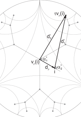
FIG. 7.: Change of coordinates in hyperbolic Poincaré disc

Note that the expression (65) does not depend on the particular representation of the hyperbolic 2-space, since the hyperbolic distance is invariant. The only one requirement is to define a compatible action of $\Gamma_{\theta}$ in the space under consideration. We use for conveniency the unit disc representation whose center is the image of the point $\nu_{\rho}(i)$ where $\nu_{\rho}$ is defined by Eq.(61) in the ${\cal H}^{2}$ representation. For shortness the generic element of $\Gamma_{\theta}$ is labelled by $\tau$ independent on the representation. We parametrize the point $\tau\nu_{\rho}(i)$ by its hyperbolic polar coordinates $(d^{\tau}_{1},\alpha^{\tau}_{1})$ with the origin at the point $i$ and by “shifted” hyperbolic coordinates $(d^{\tau}_{2},\alpha^{\tau}_{2})$ with the origin at the point $\nu_{\rho}(i)$. Note that $d_{\rho}=d(i,\nu_{\rho}(i))\sim(k+1)\ln\rho$, and the following “triangle equation” in hyperbolic 2-space holds:

$$\cosh d^{\tau}_{1}=\cosh d^{\tau}_{2}\cosh d_{\rho}+\sinh d^{\tau}_{2}\sinh d_{\rho}\cos\alpha^{\tau}_{2}$$ (B2)

In order to extract the scaling conjectured in (66), we make an approximation which consists in neglecting fluctuations of $W_{n}(d)$. In this approximation we can sum over the generations $n$ and the angles $\alpha_{j_{n}}$ of the vertices within each generation ($1\leq j_{n}\leq 3\times 2^{n-1}$). Namely $(d^{\tau}_{2},\alpha^{\tau}_{2})=(\gamma n,\alpha_{j_{n}})$. Thus one has

$$I_{{\cal N}}(\rho,q)=\sum_{n=1}^{{\cal N}}\left[2\cosh\gamma n\cosh d_{\rho}\right]^{-2q}\sum_{j_{n}=1}^{3\times 2^{n-1}}(1+\tanh\gamma n\tanh d_{\rho}\cos\alpha_{j_{n}})^{-2q}$$ (B3)

Assuming that $\alpha_{j_{n}}$ are uniformly distributed, we get for $n\gg 1$ the following expression

$$\sum_{j_{n}=1}^{3\times 2^{n-1}}(1+\tanh\gamma n\tanh d_{\rho}\cos\alpha_{j_{n}})^{-2q}\approx\frac{3\times 2^{n-1}}{2\pi}\int_{0}^{2\pi}\frac{d\alpha}{(1+\tanh\gamma n\tanh d_{\rho}\cos\alpha)^{2q}}$$ (B4)

which leads to the asymptotic behavior:

$$\left.\lim_{n\to\infty}2^{-n}\sum_{j_{n}=1}^{3\times 2^{n-1}}(1+\tanh\gamma n\tanh d_{\rho}\cos\alpha_{j_{n}})^{-2q}\right|_{\rho\to\infty}\sim\left\{\begin{array}[]{ll}{\rm const}&\mbox{for $q\leq 1/4$}\vskip 6.0pt plus 2.0pt minus 2.0pt\\ e^{2d_{\rho}(2q-\frac{1}{2})}&\mbox{for $q>1/4$}\end{array}\right.$$ (B5)

As justified hereafter we consider as relevant only the case $q\leq 1/4$. Using that for $n\gg 1$ and $\rho\gg 1$ one has $2\cosh\gamma n\cosh d_{\rho}\sim\cosh(\gamma n+d_{\rho})$ we can rewrite Eq.(B3) as follows

$$I_{{\cal N}}(\rho,q)=C\rho^{-(k+1)\ln 2/\gamma}\sum_{n=1}^{{\cal N}}2^{(n+d_{\rho}/\gamma)}[\cosh(\gamma n+d_{\rho})]^{-2q}$$ (B6)

Performing the shift $\tilde{n}=n+d_{\rho}/\gamma$ we get finally

$$I_{{\cal N}}(\rho,q)=C\rho^{-(k+1)\ln 2/\gamma}I_{{\cal N}+\frac{(k+1)}{\gamma}\ln\rho}(1,q)$$ (B7)

This expression fulfills the condition (B1). We assume that this renormalization also holds for the full function $I_{{\cal N}}(\rho,q)$.

Let us pay attention to some contradiction between (63) and (B5) raised by the set of successive approximations of (63) which however is irrelevant for our final conclusions about multifractality. The equation (63) shows that if the integral over $PSL(2,{\sf I\kern-1.49994ptR})$ converges, it should not depend on $\rho$. Using the Poincaré series, the convergence of (63) occurs for $q>q^{\star}$. For $q>1/4$ and $q>q^{\star}$ the $\rho$–dependence shown in (B5) should then cancel by summing over all $n$. The discrepancy between (63) and (B5) appears for $q\in[1/4,q^{\star}]$. First of all we should note that the interval $[\frac{1}{4},q^{\star}]$ is numerically small (following previous sections we have $q^{\star}\simeq q_{0}/2\simeq 0.4$) and is nonuniversal, i.e. depends on the particular choose of the subgroup under consideration. Moreover, both the threshold $q=1/4$ and the asymptotics (B5) depend on the distribution of $\alpha_{j_{n}}$ and we believe that more careful treatment of angle dependence in (63) would allow disregard the region $[1/4,q^{\star}]$.

REFERENCES

- [1] B.B. Mandelbrot, Multifractals and 1/f noise (Springer, 1998)
- [2] Ya. Sinai, K. Khanin, E. Vul, Sov. Mat. Uspekhi, 39, 3 (1984) (Russ.Math.Surv.)
- [3] U. Frisch, G. Parisi, in Turbulence and Predictability in Geophysical Fluid Dynamics and Climate Dynamics, Int. School of Physics ”Enrico Fermi”, Course 88, ed. M. Ghil et al (North–Holland, Amsterdam, 1985)
- [4] T. Halsey, M.Jensen, L. Kadanoff, I. Procaccia, B. Shraiman, Phys.Rev. A 33, 1141 (1986)
- [5] H. Stanley, P. Meakin, Nature 335, 405 (1988)
- [6] A. Arneodo, G. Grasseau, M. Holschneider, Phys. Rev. Lett. 61, 2281 (1988)
- [7] B. Duplantier, cond-mat/9901008
- [8] I. Kogan, C. Mudry, A. Tsvelik, Phys. Rev. Lett 77, 707 (1996); J. Caux, I. Kogan, A. Tsvelik, Nucl. Phys. B 466, 444 (1996)
- [9] C. Chamon, C. Mudry, X. Wen, Phys. Rev. Lett 77, 4196 (1996)
- [10] H. Castillo, C. Chamon, E. Fradkin, P. Goldbart, C. Mudry, Phys. Rev. B 56, 10668 (1997)
- [11] Y. Aharonov, A. Casher, Phys. Rev. D 19, 2461 (1979)
- [12] A. Comtet, Ch. Texier, cond-mat/9707313 in proc. of the workshop Supersymmetry and Integrable Models, 1997
- [13] M. Gutzwiller, B. Mandelbrot, Phys. Rev. Lett. 60, 673 (1988)
- [14] C. Series, J. London Math. Soc. (2) 31, 69 (1985)
- [15] P. Ginsparg, G. Moore, hep-th/9304011
- [16] B. Derrida, H. Spohn, J. Stat. Phys. 51, 817 (1988)
- [17] J. Gervais, A. Neveu, Nucl. Phys. B 199, 59 (1982); A. Bilal, J. Gervais, Nucl. Phys. B 305 [FS], 33 (1988)
- [18] R. Phillips, Z. Rudnik, J. Func. Anal. 121, 78 (1994)
- [19] A.B. Zamolodchikov, Al.B. Zamolodchikov, hep-th/9506136
- [20] Ch. Texier, private communication
- [21] S. Nechaev, Statistics of knots and noncommutative random walks, (WSPC: Singapore, 1996)
- [22] R. Voituriez, S. Nechaev, cond-mat/0001138
- [23] A. Terras, Harmonic Analysis on symmetric spaces and applications I (Springer, New York, 1985)
- [24] J.L. Doob, Stochastic Processes (Wiley publications in statistics, 1953)
- [25] D. Carpentier, P. Le Doussal, cond-mat/0003281
- [26] J.Elstrodt, F.Grunewald, J.Mennicke, Groups acting on hyperbolic space (Springer, 1998)
- [27] M. Sheingorn, Illinois J. Math. 24, 3 (1980)
- [28] V.I. Falko, K.B. Efetov, Phys. Rev. B 52, 24 (1995)
- [29] C. Monthus, A. Comtet, J. Phys. I 4, 635 (1994)
- [30] P. Bougerol, Probab. Th. Rel. Fields 78, 193 (1988)
- [31] J. Delsarte, Oeuvres (Editions du Centre National de la Recherche Scientifique, Paris, 1971)
- [32] K. Broderix, R. Kree, Europhys. Lett, 32, 343 (1995)
- [33] J.P. Bouchaud, A. Comtet, A. Georges, P. Le Doussal, Ann. Phys., 201, 285 (1990)
- [34] G. Oshanin, A. Mogutov, M. Moreau, J. Stat. Phys., 73, 379 (1993)
- [35] A. Comtet, C. Monthus, M. Yor, J. Appl. prob., 35, 255 (1988)
- [36] C.Texier, A. Comtet, Phys. Rev. Lett., 82, 4220 (1999)