Abstract

The Kalman filter combines forecasts and new observations to obtain an estimation which is optimal in the sense of a minimum average quadratic error. The Kalman filter has two main restrictions: (i) the dynamical system is assumed linear and (ii) forecasting errors and observational noises are projected onto Gaussian distributions. Here, we offer an important generalization to the case where errors and noises have heavy tail distributions such as power laws and Lévy laws. The main tool needed to solve this “Kalman-Lévy” filter is the “tail-covariance” matrix which generalizes the covariance matrix in the case where it is mathematically ill-defined (i.e. for power law tail exponents $\mu\leq 2$). We present the general solution and discuss its properties on pedagogical examples. The standard Kalman-Gaussian filter is recovered for the case $\mu=2$. The optimal Kalman-Lévy filter is found to deviate substantially from the standard Kalman-Gaussian filter as $\mu$ deviates from $2$. As $\mu$ decreases, novel observations are assimilated with less and less weight as a small exponent $\mu$ implies large errors with significant probabilities. In terms of implementation, the price-to-pay associated with the presence of heavy tail noise distributions is that the standard linear formalism valid for the Gaussian case is transformed into a nonlinear matrix equation for the Kalman-Lévy filter. Direct numerical experiments in the univariate case confirms our theoretical predictions.

Contents

toc

I Introduction and Motivation

The Kalman filter provides the optimal resolution of the problem of data assimilation under the hypothesis that the system observables evolve according to linear maps, are linearly related to the true variables and that the noise acting on the true dynamics and the measurement errors are mutually uncorrelated and Gaussian.

Two main limitations restrict the performance of the Kalman filter:

• the nonlinearity of the real system dynamics;

• the non-normality of the noises.

The first item has been addressed partly by using so-called “extended” Kalman filters that amount essentially to perform local linearizations [19].

With respect to the non-normality of the noises, the general condition for using the Kalman filter is that their covariance functions exist, which is satisfied for noise density distributions decaying faster than $1/x^{3}$. When the noise distributions are not Gaussian, the validity of the Kalman filter relies on the existence of a central limit theorem for state estimators, which exists when the random terms in the model have arbitrary distribution with tail decaying faster than $1/x^{3}$ [26]. For practical applications, the existence of the central limit theorem does not suffice as a finite observation time may lead to large deviations from the asymptotic results [25]. The knowledge of convergence rates in the central limit theorem are then necessary for the development of tests of the validity of the model [3].

Our purpose here is to extend these results to the regime where the existence of the covariance function is not warranted as occurs for Lévy distributions of noises, or when the covariance functions do exist but the convergence to the asymptotic result given by the central limit theorem is extremely slow making the asymptotic result useless in practice, as occurs for power law distributions [25]. In order to illustrate this idea, consider the sum of $N$ identically independent distributed random variables, with a power law probability density function $1/x^{1+\mu}$ with exponent $\mu>2$. Since the variance $\sigma^{2}$ is finite, the central limit theorem applies and the distribution of the sum converges to the Gaussian law with standard deviation $\approx\sigma\sqrt{N}$. For $N$ finite, the Gaussian law only describes the central part of the distribution of the sum, up to a cross-over $S_{0}\approx\sigma\sqrt{N\ln N}$ [25]. Beyond $S_{0}$, the distribution of the sum is a power law with the same exponent $\mu$ and the weight in probability of this power law tail decays slowly as $\propto 1/(\sqrt{N}~{}\ln^{3/2}N)$ as $N$ increases. In practice, consider the three sample sizes $N=10^{2},10^{4}$ and $10^{6}$. The corresponding cross-over values are respectively $S_{0}\approx 2.1$, $3$ and $3.7$ times the standard deviation of the central Gaussian part of the distribution of the sum. These estimates suggest that, even if the general condition for using the Kalman filter is satisfied for noise density distributions decaying faster than $1/x^{3}$, the Gaussian (or covariance) approach, which is optimal in the linear least-variance estimation, is not necessarily optimal when relatively large fluctuations (of size equal to two standard deviations or larger) occur.

We thus propose to explore how the optimal Kalman filter is modified when the objective is to minimize, not the variance of the error estimation but, a natural measure of the large errors, namely the tail of the distribution of the Euclidean norm of the errors. Our approach thus develops an alternative class of linear unbiased estimators different from the standard linear least-variance estimation. Our emphasis is in trying to control and minimize the large (and rare) errors, with the penalty that the variance, if it exists, will be sub-optimal compared to the standard linear least-variance estimation. In this goal, we focus our attention on noises in the observable and the unobservable variables both distributed with a power law tail of fixed exponent $\mu$ and known amplitudes (scale factors). This assumption offers a well-defined theoretical limit of “large fluctuations”, putting the emphasis on the complement to the “small noise” limit captured by the standard linear least-variance approach.

In addition to its pure theoretical interest, we observe that many systems in Nature are claimed to exhibit power law distributions [25] and the present results may thus have direct application. Power law distributions have been found to quantify the size-frequency Gutenberg-Richter distribution of earthquakes, of hurricanes [21], of volcanic eruptions, of floods, of meteorite sizes and so on. The distribution of seismic fault lengths is also documented to be a power law with exponent $\mu\simeq 1$. In the insurance business, recent studies has shown that the distribution of losses due to business interruption resulting from accidents [27, 28] is also a power law with $\mu\simeq 1$.

Several previous works have addressed related issues. Le Breton and Musiela’s work [17] is closest to ours but has limitations: (i) it is based on a continuous time description of the dynamical and observation processes and is thus more difficult to apply to concrete situations ; (ii) it minimizes the difference between the true dynamics and a filtered observation in the $L^{\mu}$-norm sense where $\mu$ is the index exponent of the Lévy distributions; in other words it relies on an explicit solution of the dynamics; in this way, Le Breton and Musiela circumvent the two delicate questions of generalizing the covariance matrix and of choosing the objective function to optimize; (iii) it does not really address the genuine Kalman problem which consists in mixing forecasts and observations. Recently, Ahn and Feldman [2] have proposed a filter for the case where the signal is Gaussian while the observation noise is a Lévy process. Their filter is optimal in the sense of minimizing the $L^{2}$ error, i.e. the distance between the true dynamics and the filter output. This choice of the $L^{2}$ is realizable in their case because the signal is assumed Gaussian and the integrability assumption is thus satisfied. The problem however is that the optimal filter will depend in general upon the choice of the norm that measures the prediction error. In addition, due to the rather intractable nonlinear recursive solution they obtain, they propose a sub-optimal filter for numerical purpose.

Our approach circumvents these difficulties by focusing on large errors. Our goal is thus to minimize the large errors between the analysis (obtained by assimilation of observation with prediction) and the true trajectory. With this choice, the technical problem we have to solve is to characterize the tails of error distributions, which are a function of the tail of the distributions of individual dynamical variables and of noises and of their mutual dependence. In order to determine these dependences, we propose to use the concept of a “tail-covariance” matrix that generalizes the standard covariance matrix of the analyzed signal to the case of power laws and Lévy distributions. Tail-covariance matrices are constructed as the matrices of signed scale factors (the scale factors being defined as the global amplitudes of the power law tails) of the distribution of all the products of the system and forecasted variables. The main idea is thus to replace the characterization of errors and of correlations by the ensemble of distributions of the products of all possible pairs of variables. Our approach thus replaces a reasoning based on the second centered moments into one based on the tails of the distribution of deviations from true values. It is shown that the natural error amplitude to be minimized is the trace of the tail-covariance, which is a straightforward extension of the standard approach which determines the Kalman filter by minimizing the average errors quantified by the trace of the covariance matrix of the analyzed signal.

The paper is constructed in a pedagogical manner, from the simple univariate filter problem to the full multivariate Kalman filter. In section 2, we formulate the problem for the univariate filter with power law noises, corresponding to the situation where only novel observations are assimilated without mixing with a dynamical forecast. A detailed discussion is offered to compare the power law case with the standard Gaussian case. In section 3, we generalize this problem to the case of multivariate estimators. In section 4, we address the Kalman problem of mixing both forecasts and observations with power law and Lévy law errors and develop our general solution. The special univariate case is studied in great details by numerical experiments to contrast the performances of the Kalman-Lévy with those of the standard Kalman-Gaussian filter.

II Univariate estimator: Principle of Estimation with Power Laws

A Formulation of the Problem

Take two samples $x^{\rm f}$ and $x^{\rm o}$ of an observable state variable $x$; the superscripts $\{\cdot\}^{\rm f,o}$ correspond to forecast and observation of the data assimilation system, respectively. The two samples are contaminated by independent noise $\omega^{\rm f}$ and $\omega^{\rm o}$. The estimate ${\hat{x}}$ of $x$ is sought as a linear combination of $x^{\rm o}$ and $x^{\rm f}$ with the corresponding positive weights $K^{\rm f}$ and $K^{\rm o}$

$${\hat{x}}=K^{\rm f}x^{\rm f}+K^{\rm o}x^{\rm o}~{}.$$ (1)

One of our main goals is to determine the optimal weights so as to minimize the resulting uncertainty of ${\hat{x}}$. We make two assumptions concerning samples in this study.

The first assumption that the two samples are unbiased

$$\langle x^{\rm f}\rangle=\langle x^{\rm o}\rangle=\langle x\rangle~{},$$ (2)

where $\langle z\rangle$ is the expectation of $z$. Expectation of the state variable $\langle x\rangle$ is not known a priori. By requiring further that the estimate should be unbiased $\langle{\hat{x}}\rangle=\langle x\rangle$, we obtain a relation between the two weights $K^{\rm f}+K^{\rm o}=1$ which allows us to rewrite (1) as

$${\hat{x}}=x^{\rm f}+K^{\rm o}(x^{\rm o}-x^{\rm f})~{},$$ (3)

and therefore reduces the problem to the determination of a single unknown $0\leq K^{\rm o}\leq 1$. This expression (3) can be interpreted as a filtering of the observed data $x^{\rm o}$ into the dynamical forecast $x^{\rm f}$ by a weighted increment $K^{\rm o}(x^{\rm o}-x^{\rm f})$.

The second assumption is that both sample errors,

$$\omega^{\rm f,o}=x^{\rm f,o}-x~{},$$ (4)

are distributed according to a power law as defined in (5), or according to a Lévy law as defined in Appendix A, with the same exponent $\mu^{\rm f,o}\equiv\mu$. The important property for our purpose is that the tails of the probability density functions of the two sample errors are independent and given by

$$P(\omega^{\rm f,o})\simeq{C^{\rm f,o}_{\pm}\over|\omega^{\rm f,o}|^{1+\mu}}~{}~{}~{}~{}~{}~{}~{}\mbox{ $|\omega^{\rm f,o}|\longrightarrow\pm\infty$}~{},$$ (5)

where the subscript $\{\cdot\}_{\pm}$ reflects that the tail distribution can be asymmetric depending on the sign of $\omega^{\rm f,o}$. In this study, we focus on the symmetric case, i.e., $C^{\rm f,o}_{\pm}\equiv C^{\rm f,o}$.

The family of power laws is characterized by two parameters, the exponent $\mu$ and the ‘scale factor’ $C$. The exponent $\mu$, on one hand, controls the decay rate of the probability as well as its scaling (or self-similar) properties. The scale factor $C$, on the other hand, controls the overall amplitude of the power law tail, i.e., the larger it is, the more important is the power law tail. More precisely, if the power law tail (5) holds for $\omega$ larger than some minimum value $\omega_{\rm min}^{\rm f,o}$, the weight in probability of the power law, i.e. the probability that $\omega$ is larger than $\omega_{\rm min}^{\rm f,o}$ is $(C^{\rm f,o}/\mu)(\omega_{\rm min}^{\rm f,o})^{-\mu}$. As shown in Appendix A in the case of Lévy laws, the scale parameter fully characterizes the distribution for all variations (and not only in the tail).

Notice that (5) can be rewritten in terms of the dimensionless variable $\omega/C^{1\over\mu}$ with the superscripts dropped for simplicity

$$P(\omega)d\omega\simeq{1\over|\omega/C^{1\over\mu}|^{1+\mu}}d\left(\omega/C^{1\over\mu}\right)~{}~{}~{}~{}~{}\mbox{ $|\omega|\longrightarrow\pm\infty$}~{},$$ (6)

showing that $C^{1\over\mu}$ is the characteristic scale of the self-similar fluctuations of $\omega$. For $\mu\leq 2$ (resp. $\mu\leq 1$), the variance (resp. mean) is not defined mathematically. We shall see the effect of these $\mu$-dependent properties throughout this study.

Using the continuation property given in [8] (Problem 15 of Section 12) on the characteristic function of distributions with power tails, we obtain the following results. Let us call a $\mu-$variable a variable with a distribution function with a power law tail. Then,

1. if $w_{i}$ and $w_{j}$ are two independent $\mu$-variables characterized by the scale factors $C_{i}^{\pm}$ and $C_{j}^{\pm}$, then $w_{i}+w_{j}$ is also a $\mu$-variable with $C^{\pm}$ given by $C_{i}^{\pm}+C_{j}^{\pm}$.

2. If $w$ is a $\mu$-variable with scale factor $C$, then $p\times w$ (where $p$ is a real number) is a $\mu$-variable with scale factor $p^{\mu}C$. If $p<0$ and the distribution of $w$ is symmetric, then $p\times w$ is a $\mu$-variable with scale factor $|p|^{\mu}C$.

3. If $w$ is a $\mu$-variable, then ${\rm sign}(w)|w|^{q}$, with $q>0$, is a $\mu\over q$-variable.

4. If $w_{i}$ and $w_{j}$ are two independent $\mu$-variables, then the product $x={w_{i}w_{j}}$ is also a $\mu$-variable up to logarithmic corrections.

Using the rules (i) and (ii), we find that the distribution of ${\hat{x}}$ is also a power law (5) with the same exponent $\mu$, but with an adjusted scale factor ${\hat{C}}$ given by

$${\hat{C}}=(1-K^{\rm o})^{\mu}C^{\rm f}+(K^{\rm o})^{\mu}C^{\rm o}~{}.$$ (7)

The expression (7), which is valid for $0\leq K^{\rm o}\leq 1$ such that the scale factors remain positive, can be reduced to the usual result for the Gaussian distributions [9]

$${\hat{\sigma}}^{2}=(1-K^{\rm o})^{2}(\sigma^{\rm f})^{2}+(K^{\rm o})^{2}(\sigma^{\rm o})^{2}~{},$$ (8)

by setting the exponent $\mu=2$ and replacing the scale factors $C^{\rm f,o}$ with $(\sigma^{\rm f,o})^{2}$. We thus see that the scale parameter $C$ is the generalization of the variance $\sigma^{2}$. The technical reason for this comes ¿from the form of the characteristic function of a distribution with a power law tail, as given in [8] (Problem 15 of Section 12). The situation is even simpler to discuss when considering symmetric Lévy laws whose characteristic functions read

$$\hat{L}_{\mu}(k)=\exp\left(-a_{\mu}|k|^{\mu}\right)~{},~{}~{}~{}~{}{\rm for}~{}0<\mu\leq 2~{},$$ (9)

where $a_{\mu}$ is a constant proportional to the scale parameter $C$ [11]. The important point is that, for $\mu$ strickly less than $2$, the inverse Fourier transform of $\hat{L}_{\mu}(k)$ gives a power law tail, while for $\mu=2$, it gives a Gaussian law. The continuity between the expressions (7) and (8) can thus be traced back to that of $\hat{L}_{\mu}(k)$ as a function of $\mu$ at $\mu=2$. (see Appendix A for a more formal derivation of this fact).

B Solution

The standard optimal estimation methodology consists in minimizing the variance ${\hat{\sigma}}^{2}$ with respect to the weight factor $K^{\rm o}$. The solution for $K^{\rm o}$ then gives the best weighting in the sense that we remain with the smallest uncertainty from the estimation with the novel data, by minimizing the expectation distance between ${\hat{x}}$ and $x$ in the mean-square sense. In order to generalize this methodology to the situation where the errors are distributed according to power law distributions, we propose the following central idea, i.e., to minimize the scale factor ${\hat{C}}$ with respect to $K^{\rm o}$

$$\frac{\partial{}}{\partial{K^{\rm o}}}{\hat{C}} = \mu\left[-(1-K^{\rm o})^{\mu-1}C^{\rm f}+(K^{\rm o})^{\mu-1}C^{\rm o}\right]=0$$ (10)

$$\frac{\partial{{}^{2}}}{\partial{(K^{\rm o})^{2}}}{\hat{C}} = \mu(\mu-1)\left[(1-K^{\rm o})^{\mu-2}C^{\rm f}+(K^{\rm o})^{\mu-2}C^{\rm o}\right]\geq 0.$$ (11)

The justification for this procedure is that the uncertainty in the estimation ${\hat{x}}$ of $x$ is inescapably distributed according to a power law distribution with the same exponent $\mu$ as a result of the rules (i)-(ii) given above. Consequently, the optimization using the weight $K^{o}$ can be performed only in one purpose, namely to decrease the global amplitude of the power law controlled by ${\hat{C}}$ but without be able to distort its shape defined by $\mu$. The optimal weight $K^{\rm o}$ as the solution to (10) depends on the value of the exponent $\mu$ as follows.

1. For $\mu>1$, the minimization of ${\hat{C}}$ given by (7) with respect to $K^{\rm o}$ gives

   $$K^{\rm o}={1\over 1+\lambda^{\mu\over\mu-1}}~{},$$ (12)

   where

   $$\lambda\equiv{(C^{\rm o})^{1\over\mu}\over(C^{\rm f})^{1\over\mu}}$$ (13)

   is the ratio of the characteristic error size of the two samples, as defined in the distribution (6). The resulting optimal scale factor is

   $$C^{\rm a}={\lambda^{\mu}\over\left(1+\lambda^{\mu\over\mu-1}\right)^{\mu-1}}~{}C^{\rm f}~{}$$ (14)

   where the superscript $\{\cdot\}^{\rm a}$ stands for analysis according to the data assimilation convention.

2. For $\mu<1$, there is no optimal solution for $K^{\rm o}$ which is not on the boundaries of the search interval and that minimizes ${\hat{C}}$, because $\partial^{2}{\hat{C}}/\partial(K^{\rm o})^{2}<0$ violates the second condition in (11). Physically this implies that the fluctuations are so wild that the estimation by the weighted average is not a good strategy, and that only the measurement with the smallest scale factor should be kept for the estimation of ${\hat{x}}$

   $$K^{\rm o}=\left\{\begin{array}[]{lll}0&&\mbox{for $C^{\rm o}>C^{\rm f}$}\\ 1&&\mbox{for $C^{\rm o}<C^{\rm f}$}\end{array}\right.~{},$$ (15)

   and therefore

   $$C^{\rm a}=\left\{\begin{array}[]{lll}C^{\rm f}&&\mbox{for $C^{\rm o}>C^{\rm f}$}\\ C^{\rm o}&&\mbox{for $C^{\rm o}<C^{\rm f}$}\end{array}\right.~{}.$$ (16)

   This second case $K^{\rm o}=1$, consisting in trusting observations over the forecast, is known as “direct substitution” [7]. Here, we have shown that it constitutes indeed the best strategy in the specific case $\mu\leq 1$ and $C^{\rm o}<C^{\rm f}$. Note that a similar solution applies when the two observations have different exponent $\mu$: full weight $K^{\rm o}=0$ or $1$ should be put on the observation with the largest exponent, as it has the smallest fluctuations. This solves the general case as well.

To make the problem interesting, in this paper we consider all noise sources to have the same exponent $\mu$, so that the problem is a “fight between scale-factors”. This case is not as restricted as it would appear at first site: if the mechanisms leading to the power law tail are intertwinned, such as for instance with a common source of underlying multiplicative noise, it can be shown [16, 12] that the power law exponent of the different variables will be the same as soon as there is non-vanishing coupling between the variables. This case will be investigated in a forthcoming work.

The following argument retrieves (15). When neither the variance nor the mean exist, and when the minimization (10) of the scale factor becomes meaningless, the last natural quantity to estimate is the probability that the error remaining after assimilation is smaller than the error on the two measurements. Suppose that we have the knowledge that the errors in the second measurement are larger in probability than that of the first measurement, i.e. $C^{\rm o}>C^{\rm f}$. We then require the maximization of the probability $P_{\rm improvement}$ that

$$|(1-K^{\rm o})\omega^{\rm f}+K^{\rm o}\omega^{\rm o}|\leq|\omega^{\rm f}|~{}.$$ (17)

Let us assume that $\omega^{\rm f}$ is found positive. Then, this probability is the same as the probability that

$$\left(-{2\over K^{\rm o}}+1\right)\omega^{\rm f}\leq\omega^{\rm o}\leq\omega^{\rm f}~{}.$$ (18)

The probability for (17) to be verified is thus

$$P_{\rm improvement}=2\int_{0}^{\infty}d\omega^{\rm f}P^{\rm f}(\omega^{\rm f})\int_{\left(-{2\over K^{\rm o}}+1\right)\omega^{\rm f}}^{\omega^{\rm f}}P^{\rm o}(\omega^{\rm o})d\omega^{\rm o}~{},$$ (19)

where the factor $2$ comes from the counting of the cases where $\omega^{\rm f}$ can be found negative. By taking the derivative of (19) with respect to $K^{\rm o}$, we obtain

$${dP_{\rm improvement}\over dK^{\rm o}}=-{4\over(K^{\rm o})^{2}}\int_{0}^{\infty}d\omega^{\rm f}~{}\omega^{\rm f}~{}P^{\rm f}(\omega^{\rm f})P^{\rm o}\left(\left(-{2\over K^{\rm o}}+1\right)\omega^{\rm f}\right)~{},$$ (20)

which is always negative. Thus, the probability that the error is reduced is maximum for $K^{\rm o}=0$, i.e. without assimilating the new observation. Intuitively, the power law tails with exponent $\mu<1$ are so “wild” that it is preferable to keep only the observation with the smallest scale factor. A similar derivation holds in the case where the errors in the second measurement are smaller in probability than that of the first measurement, i.e. $C^{\rm o}<C^{\rm f}$: the probability that the error is reduced is maximum for $K^{\rm o}=1$, i.e. with the assimilation of the new observation and the rejection of the first one. Again, the observation with the smaller scale factor is preferred and the other is rejected in this “wild tail” regime $\mu\leq 1$.

C Properties of the “Lévy-estimator” solution

We now examine the fundamental properties of the optimal weight $K^{\rm o}$ given by (12) which holds when the distributions of errors are pure Lévy laws as well as when they only exhibit a power law tail controlling the large variations. Figure 1 shows the influence of the tail exponent $\mu$ on the optimal weight $K^{\rm o}$ as a function of the error ratio $\lambda$ of the two measurements given by (13). As $\mu$ approaches $1$, $K^{\rm o}$ crosses over very sharply from one to zero when $\lambda$ goes through $1$, recovering the regime $\mu\leq 1$ given by (15). For larger $\mu$’s, the transition of $K^{\rm o}$ from $1$ to $0$ is smoother as $\lambda$ varies.

The result (12) for $\mu=2$ holds not only for the power law distribution itself with $\lambda=(C^{\rm o})^{1\over 2}/(C^{\rm f})^{1\over 2}$ but also for the Gaussian law distribution with the weight

$$K^{G}={1\over 1+(\lambda^{G})^{2}}~{},$$ (21)

where the superscript $\{\cdot\}^{G}$ corresponds to the Gaussian, and

$$\lambda^{G}\equiv{\sigma^{\rm o}\over\sigma^{\rm f}}~{}$$ (22)

is the ratio of the characteristic error size according to the Gaussian law. Such $K^{G}$ minimizes the variance ${\hat{\sigma}^{2}}$ given by (8). This is natural since the stable Lévy law with $\mu=2$ is nothing but the Gaussian law with the exact correspondence $C^{\rm f,o}=(\sigma^{\rm f,o})^{2}$ (see Appendix A: there should be no confusion between the exponents $\mu$ defining the characteristic functions of stable laws and the exponents $\mu$ of arbitrary power laws). Thus, the curve for $\mu=2$ in Figure 1 also applies for the Gaussian law with $K^{\rm o}=K^{G}$ and $\lambda=\lambda^{G}$. The result (12) reflects the impact of the relative uncertainties in $x^{\rm f}$ and $x^{\rm o}$ that are quantified by a parameter depending on the ratio of characteristic error size $\lambda^{{\mu\over\mu-1}}=\left(C^{\rm o}/C^{\rm f}\right)^{1\over\mu-1}$.

The weight $K^{\rm o}$ also represents the normalized increment $({\hat{x}}-x^{\rm f})$ added to the initial difference $(x^{\rm o}-x^{\rm f})$ as seen from (3):

$$K^{\rm o}={{\hat{x}}-x^{\rm f}\over x^{\rm o}-x^{\rm f}}~{}.$$ (23)

Figure 1 therefore can be interpreted as showing the normalized increment depending on the tail exponent $\mu$, with the extreme cases ${\hat{x}}=x^{\rm o}$ at $K^{\rm o}=1$ and ${\hat{x}}=x^{\rm f}$ at $K^{\rm o}=0$. At $\lambda=1$ where $x^{\rm f}$ and $x^{\rm o}$ has the same uncertainty in terms of scale factor $C^{\rm f}=C^{\rm o}$ (13), $K^{\rm o}=0.5$ puts ${\hat{x}}$ at the exact center point between $x^{\rm f}$ and $x^{\rm o}$ for any $\mu$. For $\lambda<1$ (resp.$\lambda>1$) where $x^{\rm o}$ with scale factor $C^{\rm o}$ is more (resp. less) accurate than $x^{\rm f}$ with scale factor $C^{\rm f}$, the smaller the exponent $\mu$ is, the closer ${\hat{x}}$ is to the more accurate sample $x^{\rm o}$ (resp. $x^{\rm f}$). The estimation by the weight $K^{\rm o}$ for the heavier tail distributions with $\mu<2$ therefore favors the accurate sample more strongly than in the least-variance case. Interestingly, this situation is reversed for power law tails with exponents $\mu>2$. i.e. the weight favors the accurate sample less strongly than in the Gaussian case. This situation applies in particular to exponential distributions that are formally obtained as the limit $\mu\to\infty$.

D Quality of Improvements: Lévy versus Gaussian estimators

1 Case $\mu>2$

Let us investigate the pros and cons of the solution (12) for $K^{\rm o}$ as the optimal weight for power law tails in contrast to its Gaussian counterpart (21) giving $K^{G}$. In this goal, we propose a specific example using the Student’s distribution with $\mu$ degrees of freedom, whose density function [14],

$$P_{\mu}(\omega)={\Gamma\left({\mu+1\over 2}\right)\over\sqrt{\mu\pi}~{}\Gamma\left({\mu\over 2}\right)}~{}{1/s\over\left[1+\left({\omega\over s\sqrt{\mu}}\right)^{2}\right]^{1+\mu\over 2}}~{},$$ (24)

is defined for $-\infty<\omega<+\infty$. The Student’s distribution $P_{\mu}(\omega)$ has a bell-like shape like the Gaussian (and actually tends to the Gaussian in the limit $\mu\to\infty$). It is however a power law like (5) for large $|\omega|$ with a tail exponent equal to the number $\mu$ of degrees of freedom defining the Student’s distribution, with a scale factor

$$C_{\mu}(s)={\Gamma\left({\mu+1\over 2}\right)\over\sqrt{\mu\pi}~{}\Gamma\left({\mu\over 2}\right)}~{}\mu^{1+\mu\over 2}~{}s^{\mu}~{}.$$ (25)

The parameter $s$ represents the typical width of the Student’s distribution. The variance exists only for $\mu>2$ and is given by

$${\rm Var}\equiv\sigma^{2}={\mu\over\mu-2}~{}s^{2}~{}.$$ (26)

We assume that the forecast (resp. observation) sample $x^{\rm f}$ (resp. $x^{\rm o}$) has an error $\omega^{\rm f}$ (resp. $\omega^{\rm o}$) distributed according to the student’s distribution (24) with typical width $s^{\rm f}$ (resp $s^{\rm o}$) but with the same exponent $\mu$. The Lévy weight $K^{L}$ given by (12) and the standard Gaussian weight $K^{G}$ given by (21) are represented by the same error ratio

$$\lambda^{G}=\lambda^{L}={s^{\rm o}\over s^{\rm f}}=\lambda~{}.$$ (27)

It is worth recalling that $K^{\rm o}$, which we denote here $K^{L}$, given by (12) is obtained so as to minimize the scale factor $C_{{\hat{x}}}$ given by (7), while $K^{G}$ given by (21) minimizes the variance ${\rm Var}_{{\hat{x}}}$ expressed by (8). The impact of the difference between these two weights can be quantified in several ways for $\mu>2$ where the variance exists.

One measure is the corresponding variance ${\rm Var}_{{\hat{x}}}=(1-K^{\rm o})^{2}(\sigma^{\rm f})^{2}+(K^{\rm o})^{2}(\sigma^{\rm o})^{2}$ of the total error $(1-K^{\rm o})\omega^{\rm f}+K^{\rm o}\omega^{\rm o}$ given by

$${\rm Var}_{{\hat{x}}}^{L} = {\left(1+\lambda^{2\over\mu-1}\right)\lambda^{2}\over\left(1+\lambda^{\mu\over\mu-1}\right)^{2}}(\sigma^{\rm f})^{2}$$ (28)

$${\rm Var}_{{\hat{x}}}^{G} = {\lambda^{2}\over 1+\lambda^{2}}~{}(\sigma^{\rm f})^{2}~{},$$ (29)

where ${\rm Var}_{{\hat{x}}}^{L}$ (resp. ${\rm Var}_{{\hat{x}}}^{G}$) is the variance obtained by using the solution $K^{L}$ (resp. $K^{G}$). Figure 2 shows ${\rm Var}_{{\hat{x}}}^{L}$ and ${\rm Var}_{{\hat{x}}}^{G}$ as a function of $\lambda$ for $\mu=3$: by construction, we verify that the variance of the total error is less with $K^{G}$ than with $K^{\rm o}$. This is expected since, by construction, $K^{G}$ minimizes the variance. However, the difference is small, less than $10\%$. Anyway, this measure would then suggest that the Gaussian filter is better.

However, for power law distributions of errors, the variance is well-known to be a rather poor representation of the variability, especially in the tail. It is thus interesting to compare the scale factors $C_{{\hat{x}}}^{L}$ and $C_{{\hat{x}}}^{G}$ obtained in the two schemes since they quantify the total weight of the power law tails. We determine the scale factors for the Lévy and Gaussian weights as another measure of the goodness of the filtering method:

$$C_{{\hat{x}}}^{L} = {\lambda^{\mu}\over\left(1+\lambda^{\mu\over\mu-1}\right)^{\mu-1}}C^{\rm f}~{},$$ (30)

$$C_{{\hat{x}}}^{G} = {\lambda^{\mu}\over\left(1+\lambda^{2}\right)^{\mu}(1+\lambda^{\mu})^{-1}}C^{\rm f}~{}.$$ (31)

$C_{{\hat{x}}}^{L}$ (resp. $C_{{\hat{x}}}^{G}$) is obtained by putting $K^{L}$ (resp. $K^{G}$) in expression (7). Figure 3 shows the scale factors $C_{{\hat{x}}}^{L}$ and $C_{{\hat{x}}}^{G}$ as a function of $\lambda$ for $\mu=3$: the weight $K^{L}$ is now found to be better than the usual Gaussian weight $K^{G}$, since a smaller scale factor implies smaller probabilities for large fluctuations. The improvement is however not very large, typically of the order of or less than $10\%$, i.e. of the same order as the difference between the variances (but in reverse ranking). These relatively small differences between the Gaussian and Lévy filtering procedures become enormous for the case $\mu<2$ discussed next.

The comparison between Figures 2 and 3 shows that one cannot achieve simultaneously the minimization of the variance of the error and the minimization of the weight of the tail of large deviations of the error: either one or the other can be optimized.

2 Case $\mu<2$

The situation is dramatically different when $\mu<2$, for which the variance is not mathematically defined. In this case, an empirical determination of the variance is very unstable and absolutely unreliable. The standard Gaussian weight $K^{G}$ is completely useless. In contrast, the Lévy weight $K^{L}$ gives a simple and clear-cut recipe that allows one to optimize large fluctuations in the weighting procedure.

Let us illustrate this result by the following numerical experiments using the Cauchy distribution for the errors

$$P_{C}(\omega)={1/s\over(\omega/s)^{2}+\pi^{2}}~{},$$ (32)

with typical width $s$. The Cauchy distribution (32) is one of the stable Lévy distribution and possesses a power law tail with exponent $\mu=1$ and a scale factor $C=s$. Let us assume that the first (resp. second) sample $x^{\rm f}$ (resp. $x^{\rm o}$) has an error $\omega^{\rm f}$ (resp. $\omega^{\rm o}$) distributed according to the Cauchy distribution (32) with typical width $s^{\rm f}$ (resp $s^{\rm o}$). Then, the resulting distribution of the errors on ${\hat{x}}$ is of the same form (32) with the same exponent $\mu=1$ while the scale factor is given by

$$C_{{\hat{x}}}=(1-K^{\rm o})s^{\rm f}+K^{\rm o}s^{\rm o}~{}.$$ (33)

As we have found above in (15), the weight $K^{\rm o}$ that minimizes $C_{{\hat{x}}}$ is

$$K^{\rm o}=\left\{\begin{array}[]{lll}0&&\mbox{for $s^{\rm o}>s^{\rm f}$}\\ 1&&\mbox{for $s^{\rm o}<s^{\rm f}$}\end{array}\right.,$$ (36)

since the Cauchy distribution is on the borderline $\mu=1$. This can be verified straightforwardly as a result of the linear dependence of $C_{{\hat{x}}}$ on $K^{\rm o}$ in (33) for which the optimization always selects one of the boundaries.

Consider the case where $s^{\rm f}=1$ and $s^{\rm o}=2$. The Lévy estimator imposes to choose $K^{\rm o}=0$, i.e. to reject the information provided by the second sample $x^{\rm o}$. Let us now compare this recipe with the result obtained by applying the standard Gaussian weight $K^{G}$ on data generated by using the two Cauchy laws with $s^{\rm f}=1$ and $s^{\rm o}=2$. Specifically, we generated two sets of 1000 random numbers $\omega^{\rm f}$ and $\omega^{\rm o}$, distributed according to the Cauchy law (32) with $s^{\rm f}=1$ and $s^{\rm o}=2$. From each of these 1000 numbers, we can estimate numerically the variance and find $(\sigma^{\rm f})^{2}=3.36\times 10^{5}$ and $(\sigma^{\rm o})^{2}=4.07\times 10^{5}$. The Gaussian estimator (21) then recommends the value $K^{G}=[1+(\sigma^{\rm o}/\sigma^{\rm f})^{2}]^{-1}\approx 0.45$ which is very different from $K^{\rm o}=0$ given by (36). We should stress that the estimations of the variances $(\sigma^{\rm f})^{2}$ and $(\sigma^{\rm o})^{2}$ are highly unreliable because they can change by orders of magnitude from one sample to another. The reason is, as we have said, that the variance is mathematically infinite in this case, and therefore any estimation of it is bound to be dominated by the few largest random numbers that occur by chance in the series.

Two lessons are thus to be learned from these numerical simulations: i) estimating the variance for distributions with exponent $\mu<2$ leads to very unstable results; ii) the resulting recommendation of the standard Gaussian weight $K^{G}$ can be very wrong.

III Multivariate estimator

A Definition of the model

When the state variables are multi-dimensional, their errors may be mutually dependent. If the errors are distributed according to the power or Lévy laws, we need to transform the coordinate of errors to express them as linear sums of independent noises in order to be able use the rules stated above in points (i)-(iv).

We consider a problem of estimating a multi-dimensional state vector ${\bf x}\in{\rm I\!R}^{N}$ using two samples ${\bf x}^{\rm f}\in{\rm I\!R}^{N}$ and ${\bf x}^{\rm o}\in{\rm I\!R}^{N}$. Both forecast and observations are made for all state variables. As in the case for the univariate estimation, we assume that the estimate $\hat{{\bf x}}$ of ${\bf x}$ can be expressed as a linear combination of ${\bf x}^{\rm f}$ and ${\bf x}^{\rm o}$. Requiring the unbiased condition leads to one unknown weight matrix in the estimation

$$\hat{{\bf x}}=({\bf I}-{\bf K}^{\rm o}){\bf x}^{\rm f}+{\bf K}^{\rm o}{\bf x}^{\rm o}~{},$$ (37)

where ${\bf I}$ is an identity matrix and ${\bf K}^{\rm o}\in{\rm I\!R}^{N\times N}$ is the weight matrix for the observation sample ${\bf x}^{\rm o}$. Our goal is to determine the optimal ${\bf K}^{\rm o}$ which gives the least uncertainty in $\hat{{\bf x}}$. We use the notation ${\bf K}$ for the weight matrix in connection to the standard Kalman(-Gaussian) gain matrix of sequential estimation [13].

We assume that the sample error vectors are linear sums of $N$ independent $\mu$-variables with symmetric distributions

$$\mbox{\boldmath${\epsilon}$\unboldmath}^{\rm f,o}={\bf x}^{\rm f,o}-{\bf x}={\bf G}^{\rm f,o}\mbox{\boldmath${\omega}$\unboldmath}^{\rm f,o}~{}$$ (38)

where the probability distribution of each $\omega^{\rm f,o}_{l}$ is associated with the same exponent $\mu$ and usually different individual scale factors $C^{\rm f,o}_{l}$. The assumption that the distributions of $\mbox{\boldmath${\omega}$\unboldmath}^{\rm f,o}$’s are symmetric implies that the same scale factors $C^{\rm f,o}_{l}$ characterize the tail of large positive and negative realizations. The transformation between independent $\mbox{\boldmath${\omega}$\unboldmath}^{\rm f,o}$ to mutually dependent $\mbox{\boldmath${\epsilon}$\unboldmath}^{\rm f,o}$ is provided by the matrix ${\bf G}^{\rm f,o}\in{\rm I\!R}^{N\times N}$. We shall use this decomposition scheme repeatedly in the sequel as it allows us to treat in a simple way the interplay between the power law distributions and the dependence between variables.

In the standard linear least-variance estimation theory, one calculates the covariance matrix ${\hat{\bf P}}\equiv\langle\mbox{\boldmath${\epsilon}$\unboldmath}\mbox{\boldmath${\epsilon}$\unboldmath}^{T}\rangle$ of the error $\epsilon={\hat{x}}-x$ and minimizes the expectation of the distance between $\hat{{\bf x}}$ and ${\bf x}$ in the mean-square sense, i.e., one minimizes the trace of the covariance matrix ${\hat{\bf P}}$. The covariance calculation is an essential step to guarantee that all error components are suitably accounted for. We thus propose our key idea to generalize the covariance matrix in the regime $\mu<2$ where it does not exist by using the concept of the tail-covariance defined as the matrix of scale factors of the distribution of all products $\epsilon^{\rm f,o}_{i}\epsilon^{\rm f,o}_{j}$. We prefer this approach to the so-called “co-variation” [22] as it is more intuitive and also presents nicer properties, in particular the tail-covariance matrix remains symmetric. The intuitive meaning of the co-variation is less transparent than for the tail-covariance, which explicitly measures the correlations between large events only, while the co-variation picks up contributions from the core of the distributions. Let us mention that a simplified version of the tail-covariance without signs (see below) has been used in the context of portfolio theory [4].

Consider the sample error vectors $\mbox{\boldmath${\epsilon}$\unboldmath}^{\rm f,o}$. We thus study the product $\epsilon^{\rm f,o}_{i}\epsilon^{\rm f,o}_{j}$, whose probability distribution constitutes the natural generalization of the covariance as already pointed out. Using properties (iii) and (iv) above, one finds the following result, expressed symbolically and without the superscripts for simplicity:

$$\epsilon_{i}\epsilon_{j}\simeq\sum_{l}^{N}|G_{il}||G_{jl}|\ [\mbox{${\mu\over 2}$-variable}]+\sum_{l^{\prime}}^{N}\sum_{l^{\prime\prime}\neq l^{\prime}}^{N}|G_{il^{\prime}}||G_{jl^{\prime\prime}}|\ [\mbox{${\mu}$-variable}]~{},$$ (39)

where the symbol “$\mu$-variable” defines a random variable distributed with a density distribution with a power law tail of exponent $\mu$. Expression (39) means that the tail of the distribution of the product $\epsilon_{i}\epsilon_{j}$ is dominated by the first term which has the smallest exponent $\mu/2$ and thus heaviest tail, and will directly be sensitive to the product $|G_{il}||G_{jl}|$ for all the independent errors $\omega_{l}$. More precisely, an analysis of the cumulative distribution of the products $\epsilon_{i}\epsilon_{j}$ will give an asymptotic slope of $-{\mu\over 2}$ in a log-log plot and a scale factor $C_{l}$ associated with $\omega_{l}$ proportional to $|G_{il}|^{\mu}|G_{jl}|^{\mu}$.

We use this set of scale factors associated with the distributions of $\epsilon_{i}\epsilon_{j}$ in order to define the tail-covariance matrix ${\bf B}\in{\rm I\!R}^{N\times N}$ with the following guidelines. It is natural that the tail-covariance matrix should contain the information on the tail of the products $\epsilon_{i}\epsilon_{j}$ with distribution (39). A bona-fide generalization of the covariance matrix requires two additional conditions. It should be sensitive to the sign of the dependence between the variables, i.e., if $\epsilon_{i}$ increases (resp. decreases) on average conditioned on the increase of $\epsilon_{j}$, the dependence is positive (resp. negative), generalizing the existence of positive and negative correlations. In addition, a suitable definition of the tail-covariance matrix should be such that it recovers the standard covariance matrix for the value $\mu=2$ corresponding to the special case where the stable laws reduce to the Gaussian distribution, as briefly recalled in Appendix A. These considerations lead to the following unique specification for the tail-covariance matrix by diagonalization:

$${\bf B}={\bf G}^{[{{\mu\over 2}}]}{\bf C}{\bf G}^{T[{{\mu\over 2}}]}~{}.$$ (40)

where ${\bf C}\in{\rm I\!R}^{N\times N}$ is a diagonal matrix associated with ${\omega}$ and ${\bf G}^{[{{\mu\over 2}}]}\in{\rm I\!R}^{N\times N}$ is the corresponding eigenvector matrix. The operator $\{\cdot\}^{[{\beta}]}$ means that each element of matrix or vector is defined by

$${\bf G}^{[{{\beta}}]}_{ij}={\rm sign}(G_{ij})~{}|G_{ij}|^{\beta}~{},$$ (41)

i.e., the absolute value of each element is raised to the power $\beta$ and then multiplied by its sign. This operation can be applied to scalars as well. Without the sign operator in (41), the tail-covariance matrix ${\bf B}$ would be just the matrix of scale factors of all the products $\epsilon_{i}\epsilon_{j}$. The introduction of the sign function is an essential additional ingredient introduced to account for the sign of the dependence between the variables.

For $\mu=2$, ${\bf G}^{[{{\mu\over 2}}]}_{ij}={\rm sign}(G_{ij})~{}|G_{ij}|=G_{ij}$, and we check that the tail covariance is exactly the same as the error covariance

$${\bf B}={\bf P}\equiv\langle\mbox{\boldmath${\epsilon}$\unboldmath}\mbox{\boldmath${\epsilon}$\unboldmath}^{T}\rangle~{}.$$ (42)

This correspondence may appear paradoxical if one interprets the case $\mu=2$ as corresponding to a power law, which has infinite variance. As we already discussed for the unidimensioncal case, the technical reason for this comes ¿from the form (9) of the characteristic function $\hat{L}_{\mu}(k)$ of a distribution with a power law tail, as given in [8] (Problem 15 of Section 12) or of a symmetric Lévy laws. We stress again the important point that, for $\mu$ strickly less than $2$, the inverse Fourier transform of $\hat{L}_{\mu}(k)$ defined by (9) gives a power law tail, while for $\mu=2$, it gives a Gaussian law. The continuity between the expressions (40) and (42) can thus be traced back to that of $\hat{L}_{\mu}(k)$ as a function of $\mu$ at $\mu=2$.

The transformation of the scale factors between the mutually dependent errors ${\epsilon}$ and independent errors ${\omega}$ as in (40) can be performed in both directions, i.e., not only from right- to left-hand side to compute ${\bf B}$ when ${\bf G}$ and ${\bf C}$ are known, but also from left- to right-hand side to obtain ${\bf C}$ (and ${\bf G}$) by diagonalization of ${\bf B}$.

B Solution

Our aim is to obtain the optimal weight ${\bf K}^{\rm o}$ in (37) for the best estimate $\hat{{\bf x}}$. In this goal, we form the set of products $\epsilon_{i}\epsilon_{j}$ where $\epsilon={\hat{x}}-x$ and study their probability distribution. As in (39) and (40), we retain only the term decaying as a power law with an exponent $\mu/2$ and get the following tail covariance matrix of ${\hat{\bf x}}-{\bf x}$ for an arbitrary weight matrix ${\bf K}^{\rm o}$:

$${\hat{\bf B}}=\left({\bf G}^{\rm f}-{\bf K}^{\rm o}{\bf G}^{\rm f}\right)^{[{{\mu\over 2}}]}{\bf C}^{\rm f}\left({\bf G}^{\rm f}-{\bf K}^{\rm o}{\bf G}^{\rm f}\right)^{T[{{\mu\over 2}}]}+\left({\bf K}^{\rm o}{\bf G}^{\rm o}\right)^{[{{\mu\over 2}}]}{\bf C}^{\rm o}\left({\bf K}^{\rm o}{\bf G}^{\rm o}\right)^{T[{{\mu\over 2}}]}~{}.$$ (43)

Here, we assume that errors $\mbox{\boldmath${\epsilon}$\unboldmath}^{\rm f}$ and $\mbox{\boldmath${\epsilon}$\unboldmath}^{\rm o}$ are mutually independent.

In the univariate case, the optimization process is unique and corresponds to minimizing ${\hat{C}}$ with respect to $K^{\rm o}$ as in (10). In the multivariate case, however, the optimization may be defined in several ways. For example, as recalled above, the standard linear least-variance estimation theory attempts to minimize the expectation distance between $\hat{{\bf x}}$ and ${\bf x}$ in the mean-square sense, i.e., to minimize ${\rm trace}\ {\hat{\bf P}}$ given by (42). For $\mu<2$ where the covariance ${\hat{\bf P}}$ does not exist, we propose to minimize the “average” scale factor, i.e., ${\rm trace}\ {\hat{\bf B}}$. Such an optimization implies that the uncertainty in $\hat{{\bf x}}$ is globally the smallest (see Section 2-2 for the univariate case).

Since the expression (43) is not smooth in $K^{\rm o}$ due to the presence of the absolute values, some care must be taken in the minimization. The non-smooth character of (43) makes the differentiation approach to the minimization more cumbersome, as one must keep track of the discontinuities. The optimal ${\bf K}^{\rm o}$ is obtained by solving

$$\frac{\partial{}}{\partial{{\bf K}^{\rm o}}}{\rm trace}\ {\hat{\bf B}}=0~{},$$ (44)

where

$${\hat{B}}_{ii} = \sum_{p=1}^{N}\left(G^{\rm f}_{ip}-\sum_{m=1}^{N}K^{\rm o}_{im}G^{\rm f}_{mp}\right)^{[{{\mu\over 2}}]}C^{\rm f}_{p}\left(G^{\rm f}_{ip}-\sum_{m=1}^{N}K^{\rm o}_{im}G^{\rm f}_{mp}\right)^{[{{\mu\over 2}}]}$$ (46)

$$+\sum_{p=1}^{N}\left(\sum_{m=1}^{N}K^{\rm o}_{im}G^{\rm o}_{mp}\right)^{[{{\mu\over 2}}]}C^{\rm o}_{p}\left(\sum_{m=1}^{N}K^{\rm o}_{im}G^{\rm o}_{mp}\right)^{[{{\mu\over 2}}]}$$

$$= \sum_{p=1}^{N}\left|G^{\rm f}_{ip}-\sum_{m=1}^{N}K^{\rm o}_{im}G^{\rm f}_{mp}\right|^{\mu}C^{\rm f}_{p}+\sum_{p=1}^{N}\left|\sum_{m=1}^{N}K^{\rm o}_{im}G^{\rm o}_{mp}\right|^{\mu}C^{\rm o}_{p}~{}.$$ (47)

Taking the derivative with respect to $K^{\rm o}_{ij}$, we obtain:

$$\frac{\partial{}}{\partial{K^{\rm o}_{ij}}}{\rm trace}\ {\hat{\bf B}} = \frac{\partial{}}{\partial{K^{\rm o}_{ij}}}{\hat{B}}_{ii}$$ (48)

$$= \mu\sum_{p=1}^{N}\left[-\left(G^{\rm f}_{ip}-\sum_{m=1}^{N}K^{\rm o}_{im}G^{\rm f}_{mp}\right)^{[{\mu-1}]}G^{\rm f}_{jp}C^{\rm f}_{p}\right.$$ (50)

$$\qquad+\left.\left(\sum_{m=1}^{N}K^{\rm o}_{im}G^{\rm o}_{mp}\right)^{[{\mu-1}]}G^{\rm o}_{jp}C^{\rm o}_{p}\right]=0~{},$$

where we have used the fact that $d|x|^{\mu}/dx=\mu{\rm sign}(x)~{}|x|^{\mu-1}=\mu x^{[\mu-1]}$, with our definition (41). Note that the same $N$ coefficients $K^{\rm o}_{im}$ with $m=1,...,N$ and only them occur in the $N$ equations $\frac{\partial{}}{\partial{K^{\rm o}_{ij}}}{\rm trace}\ {\hat{\bf B}}$ obtained by fixing $i$ and varying $j$ from $1$ to $N$. Finding the optimal ${\bf K}^{\rm o}$ thus involves solving $N$ independent systems of equations, one for each individual diagonal term ${\hat{B}}_{ii}$, where each system consists of the $N$ nonlinear equations $\frac{\partial{}}{\partial{K^{\rm o}_{ij}}}{\hat{B}}_{ii}=0$ for the $N$ unknowns $K^{\rm o}_{ij}$ at $i$ fixed.

Optimality of ${\bf K}^{\rm o}$ is ensured by the positive definiteness of the Hessian matrix for ${\hat{B}}_{ii}$ with respect to $K^{\rm o}_{ij}$, for each of the $N$ independent systems (each defined as we have shown by a fixed $i$) of $N$ equations (obtained by varying $j$ at fixed $i$). While for the univariate case, this amounts to ensure the validity of only one equation (11), in the multivariate case we need to study the positive definiteness of the Hessian:

$$\frac{\partial{{}^{2}}}{\partial{(K^{\rm o}_{ij})\partial(K^{\rm o}_{iq})}}{\hat{B}}_{ii}= \mu(\mu-1) \left[\sum_{p=1}^{N}(G^{\rm f}_{jp})(G^{\rm f}_{qp})\left|G^{\rm f}_{ip}-\sum_{m=1}^{N}K^{\rm o}_{im}G^{\rm f}_{mp}\right|^{\mu-2}C^{\rm f}_{p}\right.$$ (52)

$$\left.+\sum_{p=1}^{N}(G^{\rm o}_{jp})(G^{\rm o}_{qp})\left|\sum_{m=1}^{N}K^{\rm o}_{im}G^{\rm o}_{mp}\right|^{\mu-2}C^{\rm o}_{p}\right]~{},$$

expressed at the values of ${\bf K}^{\rm o}$ solving (50). If this matrix is positive definite, then $K^{\rm o}_{ij}$ minimizes ${\hat{B}}_{ii}$ and is therefore optimal. There are two issues associated with this formulation for the optimal ${\kappa}$ (i.e., ${\bf K}^{\rm o}$): 1) the possible existence of singular terms for $\mu<2$; and 2) the solvability of the nonlinear system. We address them in the appendix B and show that the matrix is indeed positive definite and that there is only one solution.

C Special cases

1 Case $\mu=2$

For $\mu=2$, the Lévy estimator is the same as the Gaussian one which minimizes ${\rm trace}\ {\hat{\bf P}}={\rm trace}\ {\hat{\bf B}}$ as given by (42). In this case, the system becomes perfectly linear with ${\mu\over 2}=\mu-1=1$ and leads to the following analytical solution for the optimal weight given in matrix form

$${\bf K}^{G}={\bf B}^{\rm f}\left({\bf B}^{\rm f}+{\bf B}^{\rm o}\right)^{-1}~{},$$ (53)

which results in the optimal estimates of the state variable and corresponding covariance matrix

$${\hat{\bf x}}^{G} = {\bf B}^{\rm o}\left({\bf B}^{\rm f}+{\bf B}^{\rm o}\right)^{-1}{\bf x}^{\rm o}+{\bf B}^{\rm f}\left({\bf B}^{\rm f}+{\bf B}^{\rm o}\right)^{-1}{\bf x}^{\rm f}~{},$$ (54)

$${\hat{\bf B}}^{G} = {\bf B}^{\rm o}\left({\bf B}^{\rm f}+{\bf B}^{\rm o}\right)^{-1}{\bf B}^{\rm f}~{}.$$ (55)

2 Independent noise

When the errors $\mbox{\boldmath${\epsilon}$\unboldmath}^{\rm f,o}$ are independent, i.e., ${\bf G}^{\rm f,o}={\bf I}$, the trace and diagonal components (46) for the average scale factor can be simplified into

$${\rm trace}\ {\hat{\bf B}}=\sum_{i=1}^{N}\sum_{p=1}^{N}\left[\left(1-K^{\rm o}_{ip}\right)^{\mu}C^{\rm f}_{p}+\left(K^{\rm o}_{ip}\right)^{\mu}C^{\rm o}_{p}\right]~{},$$ (56)

where we have omitted the absolute values and the sign functions as we look for values of the Kalman weights between $0$ and $1$. Therefore, the problem can be reduced to the univariate estimate for each element $x_{i}$ independently, as defined in equation (7). The equations (10,11) are thus replaced by their exact equivalent derived from the two conditions (44) and (52). The solution $K^{\rm o}_{ii}$ for each $i$ is given by (12) where $K^{\rm o}_{ii}=K^{\rm o}$ is obtained by setting $\lambda=(C^{\rm o}_{i})^{1\over\mu}/(C^{\rm f}_{i})^{1\over\mu}$ (see (13)). Due to the hypothesis of noise independence, the non-diagonal coefficients $K^{\rm o}_{ij}$ are all zero for $i\neq j$.

IV The Kalman-Lévy filter

A Problem

We are now in a position to construct a sequential data assimilation methodology when the noises are distributed according to the power or Lévy law. The standard assimilation problem is formulated as follows. We consider a linear discrete stochastic dynamical system of state variables ${\bf x}\in{\rm I\!R}^{N}$

$${\bf x}_{k}^{\rm t}={\bf M}_{k,k-1}{\bf x}_{k-1}^{\rm t}+\mbox{\boldmath${\eta}$\unboldmath}_{k-1}^{\rm t}~{},$$ (57)

where superscript $\{\cdot\}^{\rm t}$ denotes the true state and $\mbox{\boldmath${\eta}$\unboldmath}_{k-1}^{\rm t}$ is the dynamical noise. The index $k$ corresponds to the time sequence when the observations ${\bf y}_{k}^{\rm o}\in{\rm I\!R}^{L_{k}}$ are taken as

$${\bf y}_{k}^{\rm o}={\bf H}_{k}{\bf x}_{k}^{\rm t}+\mbox{\boldmath${\epsilon}$\unboldmath}_{k}^{\rm o}~{},$$ (58)

where $\mbox{\boldmath${\epsilon}$\unboldmath}_{k}^{\rm o}$ is the observational noise and ${\bf H}_{k}\in{\rm I\!R}^{L_{k}\times N}$ is the linear observation function which can vary at each time step $k$. These observations ${\bf y}_{k}^{\rm o}$ are assumed to be linear functions of the state variable ${\bf x}_{k}^{\rm t}$ of the system with an additive noise.

The estimation methodology developed in the previous sections is now extended to perform a filtering in order to estimate ${\bf x}^{\rm t}$ sequentially, by assimilating ${\bf y}_{k}^{\rm o}$ into the deterministic forecast ${\bf x}_{k}^{\rm f}$. Here, we assume that ${\bf M}_{k,k-1}$ and ${\bf H}_{k}$ are known. The assimilation cycle $k$ is defined over a time interval $[k-1,k]$ between the two adjacent observation events. It consists of the following two steps:

1. a deterministic forecast ${\bf x}_{k}^{\rm f}$ of ${\bf x}_{k}^{\rm t}$ from a given initial condition ${\bf x}_{k-1}^{\rm a}$ as the best estimate of ${\bf x}_{k-1}^{\rm t}$ based on the model

   $${\bf x}_{k}^{\rm f}={\bf M}_{k,k-1}{\bf x}_{k-1}^{\rm a}~{}.$$ (59)

   The forecast is based on the analysis performed at the previous time step.

2. This forecast is then used to construct the new analysis ${\bf x}_{k}^{\rm a}$ which is mixed with the assimilated observation. This leads to the probabilistic analysis ${\bf x}_{k}^{\rm a}$ of ${\bf x}_{k}^{\rm t}$ obtained as the weighted average of ${\bf x}_{k}^{\rm f}$ and ${\bf y}_{k}^{\rm o}$ under the unbias assumption at time $k$:

   $${\bf x}_{k}^{\rm a}={\bf x}_{k}^{\rm f}+{\bf K}_{k}\left({\bf y}_{k}^{\rm o}-{\bf H}_{k}{\bf x}_{k}^{\rm f}\right)=\left({\bf I}-{\bf K}_{k}{\bf H}_{k}\right){\bf x}_{k}^{\rm f}+{\bf K}_{k}{\bf y}_{k}^{\rm o}~{}.$$ (60)

Accordingly, the errors associated with ${\bf x}_{k}^{\rm f}$ and ${\bf x}_{k}^{\rm a}$ are auto-regressive processes.

$${\bf x}_{k}^{\rm f}-{\bf x}_{k}^{\rm t} = {\bf M}_{k,k-1}\left({\bf x}_{k-1}^{\rm a}-{\bf x}_{k-1}^{\rm t}\right)-\mbox{\boldmath${\eta}$\unboldmath}_{k-1}^{\rm t}~{},$$ (61)

$${\bf x}_{k}^{\rm a}-{\bf x}_{k}^{\rm t} = \left({\bf I}-{\bf K}_{k}{\bf H}_{k}\right)\left({\bf x}_{k}^{\rm f}-{\bf x}_{k}^{\rm t}\right)+{\bf K}_{k}\mbox{\boldmath${\epsilon}$\unboldmath}_{k}^{\rm o}$$ (62)

$$= \left({\bf I}-{\bf K}_{k}{\bf H}_{k}\right){\bf M}_{k,k-1}\left({\bf x}_{k-1}^{\rm a}-{\bf x}_{k-1}^{\rm t}\right)-\left({\bf I}-{\bf K}_{k}{\bf H}_{k}\right)\mbox{\boldmath${\eta}$\unboldmath}_{k-1}^{\rm t}+{\bf K}_{k}\mbox{\boldmath${\epsilon}$\unboldmath}_{k}^{\rm o}$$ (63)

and the only unknown to be determined is the so-called “gain matrix” ${\bf K}_{k}$ needed in order to complete the assimilation cycle.

Our goal is therefore to determine the gain matrix ${\bf K}_{k}^{L}$, where the superscript $L$ refers to the Kalman-Lévy filter, which results in the least uncertainty in ${\bf x}_{k}^{\rm a}$ in each assimilation cycle when the noises are distributed according to the power or Lévy law with the exponent $\mu$. As in (38), we express the sample error vectors as linear sums of $N$ independent $\mu$-variables

$$\mbox{\boldmath${\eta}$\unboldmath}_{k}\equiv{\bf G}_{k}^{\eta}\mbox{\boldmath${\omega}$\unboldmath}_{k}^{\eta},\qquad\mbox{\boldmath${\epsilon}$\unboldmath}_{k}\equiv{\bf G}_{k}^{\epsilon}\mbox{\boldmath${\omega}$\unboldmath}_{k}^{\epsilon}~{}.$$ (64)

Because (61) and (63) define linear autoregressive processes with Lévy-stable or power law probability distribution of the noises, the errors in forecast and analysis are also distributed according to the power or Lévy laws with the same exponent $\mu$. Without loss of generality, they can thus be written as

$${\bf x}_{k}^{\rm f,a}-\hat{{\bf x}}_{k}\equiv{\bf G}_{k}^{\rm f,a}\mbox{\boldmath${\omega}$\unboldmath}_{k}^{\rm f,a}~{},\\$$ (65)

which defines the matrices ${\bf G}_{k}^{\rm f,a}$ and the vectors $\mbox{\boldmath${\omega}$\unboldmath}_{k}^{\rm f,a}$ of independent Lévy or power law processes. Consequently, all error and noise distributions in the assimilation cycles are characterized by the corresponding tail covariance matrices

$${\bf B}_{k}^{\rm f,a} \equiv \left({\bf G}_{k}^{\rm f,a}\right)^{[{{\mu\over 2}}]}{\bf C}_{k}^{\rm f,a}\left({\bf G}_{k}^{\rm f,a}\right)^{T[{{\mu\over 2}}]}$$ (66)

$${\bf B}_{k}^{\eta,\epsilon} \equiv \left({\bf G}_{k}^{\eta,\epsilon}\right)^{[{{\mu\over 2}}]}{\bf C}_{k}^{\eta,\epsilon}\left({\bf G}_{k}^{\eta,\epsilon}\right)^{T[{{\mu\over 2}}]}~{},$$ (67)

where ${\bf C}\in{\rm I\!R}^{N\times N}$ is a diagonal scale-factor matrix associated with ${\omega}$ and ${\bf G}^{[{{\mu\over 2}}]}$ is the corresponding eigenvector matrix. Given a ${\bf B}$, the corresponding ${\bf G}$ and ${\bf C}$ can be obtained by diagonalization.

B Solution

The optimal Kalman-Lévy (KL) filter ${\bf K}_{k}^{L}$ which minimizes the global average error is obtained by minimizing the trace of the tail-covariance matrix ${\bf B}_{k}^{\rm a}$ of the resulting probabilistic analysis ${\bf x}_{k}^{\rm a}$ of ${\bf x}_{k}^{\rm t}$. Since the expression for ${\bf B}_{k}^{\rm a}$ is not smooth in ${\bf K}_{k}^{L}$ due to the presence of the absolute values, some care must be taken in the minimization as already discussed. The non-smooth character of ${\bf B}_{k}^{\rm a}$ makes the differentiation approach to the minimization more cumbersome, as one must keep track of the discontinuities. However, we use the approach described in Appendix B to check if the two conditions are simultaneously verified:

$$\frac{\partial{}}{\partial{{\bf K}_{k}^{L}}}{\rm trace}{\bf B}_{k}^{\rm a}=0~{},$$ (68)

and positive-definiteness of the Hessian matrix

$$\frac{\partial{{}^{2}}}{\partial{({\bf K}_{k}^{L})^{2}}}{\rm trace}{\bf B}_{k}^{\rm a}~{}.$$ (69)

We solve the first condition and then examine the second condition. This is achieved by taking the following two steps in each assimilation cycle.

• Dynamic forecast:
  Given a set of initial conditions described by the subscript $\{\cdot\}_{k-1}$ which are known, the forecast is performed deterministically to advance from $k-1$ to $k$ based on (59) and (61)

  $${\bf x}_{k}^{\rm f}={\bf M}_{k,k-1}{\bf x}_{k-1}^{\rm a}$$ (70)

  leading to the tail-covariance of the forecasts at time $k$:

  $${\bf B}_{k}^{\rm f}=\left({\bf M}_{k,k-1}{\bf G}_{k-1}^{\rm a}\right)^{[{{\mu\over 2}}]}{\bf C}_{k-1}^{\rm a}\left({\bf M}_{k,k-1}{\bf G}_{k-1}^{\rm a}\right)^{T[{{\mu\over 2}}]}+{\bf B}_{k-1}^{\eta}~{},$$ (71)

  where the definition (40,41) is used.

• Probabilistic analysis:
  Given the forecast ${\bf x}_{k}^{\rm f}$ with ${\bf B}_{k}^{\rm f}$ from Step 1 along with the observations ${\bf y}_{k}^{\rm o}$ with tail-covariance ${\bf B}_{k}^{\epsilon}$, the analysis provides the optimal estimate

  $${\bf x}_{k}^{\rm a}={\bf x}_{k}^{\rm f}+{\bf K}_{k}^{L}\left({\bf y}_{k}^{\rm o}-{\bf H}_{k}{\bf x}_{k}^{\rm f}\right)~{}$$ (72)

  with tail-covariance

  $${\bf B}_{k}^{\rm a} = \left({\bf G}_{k}^{\rm f}-{\bf K}_{k}^{L}{\bf H}_{k}{\bf G}_{k}^{\rm f}\right)^{[{{\mu\over 2}}]}{\bf C}_{k}^{\rm f}\left({\bf G}_{k}^{\rm f}-{\bf K}_{k}^{L}{\bf H}_{k}{\bf G}_{k}^{\rm f}\right)^{T[{{\mu\over 2}}]}$$ (74)

  $$+\left({\bf K}_{k}^{L}{\bf G}_{k}^{\epsilon}\right)^{[{{\mu\over 2}}]}{\bf C}_{k}^{\epsilon}\left({\bf K}_{k}^{L}{\bf G}_{k}^{\epsilon}\right)^{T[{{\mu\over 2}}]}~{},$$

  where the definition (40,41) is used. By letting subscripts represent the matrix elements and dropping the time index $k$ for simplicity, we solve for the optimal filter ${\bf K}^{L}$ so that it satisfies the conditions (68). The diagonal elements of $B^{\rm a}$ can be explicated as follows:

  $$B^{\rm a}_{ii} = \sum_{p=1}^{N}\left|G^{\rm f}_{ip}-\sum_{m=1}^{L}K_{im}H^{{\bf G}}_{mp}\right|^{\mu}C^{\rm f}_{p}+\sum_{q=1}^{L}\left|\sum_{m=1}^{L}K_{im}G^{\epsilon}_{mq}\right|^{\mu}C^{\epsilon}_{q}~{},$$ (75)

  with

  $${\bf H}^{{\bf G}}\equiv{\bf H}{\bf G}^{\rm f}~{}.$$ (76)

  Because $B^{\rm a}_{ii}$ does not depend on $K_{qj}$ for $q\neq i$, the first condition for the optimal ${\bf K}_{k}^{L}$ (68) is

  $$\frac{\partial{}}{\partial{K^{L}_{ij}}}{\rm trace}\ {\bf B}^{\rm a} = \frac{\partial{}}{\partial{K^{L}_{ij}}}B^{\rm a}_{ii}=0$$ (77)

  $$= \mu\left[-\sum_{p=1}^{N}\left(G^{\rm f}_{ip}-\sum_{m=1}^{L}K^{L}_{im}H^{{\bf G}}_{mp}\right)^{[{\mu-1}]}H^{{\bf G}}_{jp}C^{\rm f}_{p}\right.$$ (79)

  $$+\left.\sum_{q=1}^{L}\left(\sum_{m=1}^{L}K^{L}_{im}G^{\epsilon}_{mq}\right)^{[{\mu-1}]}G^{\epsilon}_{jq}C^{\epsilon}_{q}\right]=0~{},$$

  using the signed power operator as in the case of (50).

  For the optimal filter ${\bf K}^{L}$ so obtained, positive definitiveness of the Hessian matrix

  $$\frac{\partial{{}^{2}}}{\partial{(K^{\rm L}_{ij})\partial(K^{\rm L}_{iq})}}{\rm trace}\ {\bf B}^{\rm a} = \frac{\partial{{}^{2}}}{\partial{(K^{\rm L}_{ij})\partial(K^{\rm L}_{iq})}}B^{\rm a}_{ii}$$ (80)

  $$= \mu(\mu-1)\left[\sum_{p=1}^{N}\left|G^{\rm f}_{ip}-\sum_{m=1}^{L}K^{L}_{im}G^{\epsilon}_{mp}\right|^{\mu-2}(H^{{\bf G}}_{jp})(H^{{\bf G}}_{qp})C^{\rm f}_{p}\right.$$ (82)

  $$+\left.\sum_{q=1}^{L}\left|\sum_{m=1}^{L}K^{L}_{im}G^{\epsilon}_{mq}\right|^{\mu-2}(G^{\epsilon}_{jp})G^{\epsilon}_{qp}C^{\epsilon}_{q}\right]~{},$$

  is satisfied for $\mu>1$, following the same approach as discussed in Section 3-2 and in Appendix B.

  The optimal estimate ${\bf x}_{k}^{\rm a}$ and tail-covariance ${\bf B}_{k}^{\rm a}$ obtained by substituting ${\bf K}_{k}^{L}$ into (72) and (74) become a set of initial conditions for the next assimilation cycle $k+1$.

Similarly to the case of the multivariate estimator which is solution of (50) discussed in Section III B, the first condition for the optimal KL filter (77) for a fixed $i$ leads to a set of $N$ self-contained nonlinear equations for $N$ unknowns for $j=1,\ldots,N$. Minimization of the average scale factor is therefore equivalent to the minimization of each tail-covariance element $B^{\rm a}_{ii}$ for $x^{\rm a}_{i}-x^{\rm t}_{i}$ with respect to the elements of ${\bf K}_{k}$ with at least one of the indexes equal to $i$. Such a set of solutions of the nonlinear equations for an arbitrary $\mu$ may not be available analytically but can be obtained numerically. For $\mu=2$, the KL filter is reduced to the same formula as the conventional Kalman-Gaussian (KG) filter, i.e., the forecast error tail-covariance (71) is

$${\bf B}_{k}^{\rm f}={\bf M}_{k,k-1}{\bf B}_{k-1}^{\rm a}{\bf M}_{k,k-1}^{T}+{\bf B}_{k-1}^{\eta}~{}.$$ (83)

The analysis error tail-covariance (74) is

$${\bf B}_{k}^{\rm a} = \left({\bf I}-{\bf K}_{k}^{G}{\bf H}_{k}\right){\bf B}_{k}^{\rm f}~{},$$ (84)

where the optimal KG gain that satisfies (68) is given by

$${\bf K}_{k}^{G}={\bf B}_{k}^{\rm f}{\bf H}_{k}^{T}\left({\bf H}_{k}{\bf B}_{k}^{\rm f}{\bf H}_{k}^{T}+{\bf B}_{k}^{\epsilon}\right)^{-1}~{}.$$ (85)

The analysis state variable ${\bf x}_{k}^{\rm a}$ is also obtained by substituting (85) into (72). In this case, sequential data assimilation does not require any diagonalization of the tail covariance matrix.

C Univariate Kalman-Lévy filter

1 Solution

To understand the fundamental properties of the KL filter, we study the univariate problem with $N=1$ and $L=1$ in detail for the case where the exponent $\mu$ is larger than $1$. The case $\mu\leq 1$ has been discussed in section 2 and leads to a Kalman weight equal to either $0$ or $1$.

In this case, the tail-covariances $B^{{\rm f,a,t}}$ correspond to the scale factors $C^{{\rm f,a,t}}$ directly and we have the following data assimilation cycle.

• Dynamic forecast:

  $$x^{\rm f}_{k}=M_{k,k-1}x^{\rm a}_{k-1}$$ (86)

  with tail-covariance matrix

  $$B_{k}^{\rm f}=|M_{k,k-1}|^{\mu}B_{k-1}^{\rm a}+B_{k-1}^{\eta}$$ (87)

  as derived from (61) using the calculation rules given above in points (i)-(iv).

• Probabilistic analysis:
  

  $$x^{\rm a}_{k}=\left(1-K_{k}H_{k}\right)x^{\rm f}_{k}+K_{k}y_{k}^{\rm o}~{},$$ (88)

  leading to the following scale factor

  $$B_{k}^{\rm a}=\left|1-K_{k}H_{k}\right|^{\mu}B_{k}^{\rm f}+|K_{k}|^{\mu}B_{k}^{\epsilon}~{}.$$ (89)

  Its minimization with respect to $K_{k}$ leads to

  $$x^{\rm a}_{k} = {(\lambda_{k}^{H})^{{\mu\over\mu-1}}\over 1+(\lambda_{k}^{H})^{{\mu\over\mu-1}}}x^{\rm f}_{k}+{{H_{k}}^{-1}\over 1+(\lambda_{k}^{H})^{{\mu\over\mu-1}}}y_{k}^{\rm o}$$ (90)

  $$B_{k}^{\rm a} = {(\lambda_{k}^{H})^{\mu}\over\left[1+(\lambda_{k}^{H})^{{\mu\over\mu-1}}\right]^{\mu-1}}B_{k}^{\rm f}~{},$$ (91)

  after substituting the optimal KL gain

  $$K_{k}^{L}={{H_{k}}^{-1}\over 1+(\lambda_{k}^{H})^{{\mu\over\mu-1}}}~{},$$ (92)

  with the modified relative error ratio

  $$\lambda_{k}^{H}\equiv{\lambda_{k}\over H_{k}}={(B_{k}^{\epsilon})^{{1\over\mu}}\over H_{k}(B_{k}^{\rm f})^{{1\over\mu}}}~{}.$$ (93)

  Notice that expression (91) is nothing but rewriting (14).

2 Properties of the solution

Because the KL filter is designed to minimize $B_{k}^{\rm a}$, we gain insight into its performance by investigating $B_{k}^{\rm a}$ along with $B_{k}^{\rm f}$ in each assimilation cycle. While the state variable $x_{k}^{\rm f,a}$ has a stochastic dynamics through the observation $y^{\rm o}$, their scale factors $B_{k}^{\rm f,a}$ are completely deterministic. Using (91) and (87), the evolution of $B_{k}^{\rm f,a}$ can be expressed as uncoupled one-dimensional maps:

$$B_{k}^{\rm f} = {|M_{k,k-1}\lambda_{k-1}^{H}|^{\mu}\over\left[1+(\lambda_{k-1}^{H})^{{\mu\over\mu-1}}\right]^{\mu-1}}B_{k-1}^{\rm f}+B_{k-1}^{\eta}~{}$$ (94)

$$B_{k}^{\rm a} = {(\lambda_{k}^{H})^{\mu}\over\left[1+(\lambda_{k}^{H})^{{\mu\over\mu-1}}\right]^{\mu-1}}\left[|M_{k,k-1}|^{\mu}B_{k-1}^{\rm a}+B_{k-1}^{\eta}\right]~{},$$ (95)

where $\lambda_{k}^{H}$ in $B_{k}^{\rm a}$ can be given in terms of $B_{k-1}^{\rm a}$ for (95) by substitution of (87) into (93).

Two limiting cases can be analyzed. First, in the limit where the main origin of variability in the factor $F$ multiplying $B_{k-1}^{\rm f}$ in the r.h.s. of (94) comes from either $M_{k,k-1}$, $B_{k}^{\epsilon}$ or $H_{k}$ and not from $B_{k}^{\rm f}$, this factor $F$ can be considered to be approximately independent of $B_{k-1}^{\rm f}$. The expression (94) becomes a multiplicative noisy auto-regressive equation which has been much studied in the literature [16, 6, 24, 23]. The most important result is that $B_{k}^{\rm f}$ remains finite at all times if the expectation of the logarithm of the factor $F$ multiplying $B_{k-1}^{\rm f}$ in (94) is negative. This condition ensures that $B_{k}^{\rm f}$ does not grow exponentially at large times. Usually, in this regime, if the factor $F$ exhibits intermittent excursions to values larger than one, it can be shown that the scale factors $B_{k-1}^{\rm f}$ themselves will be distributed according to a power law distribution. A similar result holds for $B_{k}^{\rm a}$, whose upper limit is bounded by $B_{k}^{\rm f}$.

The second interesting case occurs when the system is stationary, i.e., $M=M_{k,k-1}$, $H=H_{k}$, and $B^{\eta,\epsilon}=B_{k}^{\eta,\epsilon}$ for all $k$. By defining nondimensional tail-covariances (which are replaced by scale factors in this single variable case) normalized by the dynamical error’s scale factor $B^{\eta}$,

$$b_{k}^{\rm f,a}={B_{k}^{\rm f,a}\over B^{\eta}}~{},$$ (96)

the corresponding dynamical maps (94) and (95) are reduced into

$$b_{k}^{\rm f} = {|M\lambda^{b}|^{\mu}\over\left\{1+\left[{\lambda^{b}\over(b_{k-1}^{\rm f})^{{1\over\mu}}}\right]^{{\mu\over\mu-1}}\right\}^{\mu-1}}~{}+1~{},$$ (97)

$$b_{k}^{\rm a} = {(\lambda^{b})^{\mu}\over\left\{1+\left[{\lambda^{b}\over(|M|^{\mu}b_{k-1}^{\rm a}+1)^{{1\over\mu}}}\right]^{{\mu\over\mu-1}}\right\}^{\mu-1}}~{}.$$ (98)

For a given $\mu$, the two parameters controlling the evolution of $b_{k}^{\rm f,a}$ are the dynamical coefficient $M$ and the ratio of the characteristic error sizes of the dynamics over the observation defined by

$$\lambda^{b} \equiv {1\over H}{(B^{\epsilon})^{1\over\mu}\over(B^{\eta})^{1\over\mu}}~{}.$$ (99)

The corresponding KL gain is

$$K_{k}^{L}={H^{-1}\over 1+\left[{\lambda^{b}\over(b_{k-1}^{\rm f})^{{1\over\mu}}}\right]^{{\mu\over\mu-1}}}~{},$$ (100)

which can be expressed in terms of $b_{k-1}^{\rm a}$ as well. The KL filter parameter (99) and gain (100) are the counterpart of (13) and (12), and the resulting KL analysis (98) takes the form similar to (14) of the Lévy estimator in Section II B.

For any values of $b_{k-1}^{\rm f,a}$, the scale factors $b_{k}^{\rm f,a}$ at the next time step are bounded:

$$1< b_{k}^{\rm f} <|M\lambda^{b}|^{\mu}+1$$ (101)

$${(\lambda^{b})^{\mu}\over\left[1+(\lambda^{b})^{{\mu\over\mu-1}}\right]^{\mu-1}}< b_{k}^{\rm a} <(\lambda^{b})^{\mu}~{},$$ (102)

indicating that the univariate sequential estimation system cannot diverge as long as the exponent $\mu$ is finite.

The evolution of the scale factors is demonstrated in Figure 4a. The maps are represented by the graphs of $b_{k}^{\rm f}$ and $b_{k}^{\rm a}$ as functions of $b_{k-1}^{\rm a}$ for four values of the exponent $\mu=1.2,1.5,2$ and $3$ with the set of parameters $(\lambda^{b},M)=(1,0.9)$, corresponding to a contracting map. Starting from $b_{k-1}^{\rm a}$ on the diagonal line, the dynamic forecast takes $b_{k-1}^{\rm a}$ to $b_{k}^{\rm f}$ on the corresponding $\mu$-curve (upper group), which is followed by the probabilistic analysis down to $b_{k}^{\rm a}$ on the corresponding $\mu$-curve (lower group) to complete one data assimilation cycle, $b_{k-1}^{\rm a}\to b_{k}^{\rm f}\to b_{k}^{\rm a}$. A new analysis $b_{k}^{\rm a}$ is moved horizontally onto the diagonal line to become an initial scale factor value for the next cycle.

On each $b_{k}^{\rm a}$ curve for a fixed $\mu$, the symbols (circle, square, diamond and triangle for $\mu=1.2,1.5,2$ and $3$, respectively) at the intersection with the diagonal line, i.e. $\bar{b}^{\rm a}=b_{k}^{\rm a}=b_{k-1}^{\rm a}$, are the stable solutions of the KL filter. The maps (97) and (98) in fact have each a stable fixed-point solution, $\bar{b}^{\rm f}$ and $\bar{b}^{\rm a}$, that attracts any initial condition for any exponent $\mu$, given a set of parameters $(\lambda^{b},M)$. For $\mu=2$ retrieving the case of the KG filter, this stable fixed-point can be obtained analytically[10].

The error probability distributions for the stable fixed-points corresponding to the Student’s distribution (24) are shown in Figure 4b–e based on the scale factor $\bar{b}^{\rm f,a}$. We use $(x^{\rm f},y^{\rm o})=(0,1)$ and $H=1$, so that $x^{\rm a}=K^{L}$. For small $\mu$, the KL filter favors more strongly the better sample characterized by the smaller scale factor between the two ($\bar{b}^{\rm f}$ for $x^{\rm f}$ and $(\lambda^{b})^{\mu}$ for $y^{\rm o}$). This effect is stronger when $\mu$ decreases to $1$, as discussed in section 2. The value of the fixed point $\bar{b}^{\rm a}$ is larger for smaller $\mu$, i.e., a system with a probability distribution with heavier tail has greater uncertainty, not only because of its slow decay measured by the exponent $\mu$ but also due to its overall amplitude quantified by the scale factor. Furthermore, the slope of the curve $b_{k}^{\rm a}$ as a function of $b_{k-1}^{a}$ shown in Figure 4 is closer to the horizontal for smaller $\mu$, indicating that the convergence to the stable fixed-point is faster for the heavy-tail probability distribution. This is because the KL filter with smaller $\mu$ tends to favor either forecast or observation strongly, depending on their relative noise amplitude quantified by the scale factor of their noises, as discussed in Section II C.

Since the stationary KL assimilation system quickly approaches a unique steady state for a given set of parameters $(\lambda^{b},M)$ and exponent $\mu$, the stable fixed-point defined by $\bar{b}^{\rm f}$ and $\bar{b}^{\rm a}$ along with the corresponding optimal Kalman-Lévy gain $\bar{K}^{L}$ suffice to provide a complete description of the stationary assimilation process. Figure 5 shows the stable solution obtained from (97), (98) and (100), which are plotted in the parameter space $(\lambda^{b},M)$ for $\mu=1.2,1.5$ and $2$. All tail covariances (scale factors) are plotted in terms of $(\bar{b})^{{1\over\mu}}$ so as to preserve the characteristic scale as in (6) of the error, independently of the value of $\mu$.

For convergent dynamics $M<1$ with sufficiently large relative observational error $\lambda^{b}>1$, $\lambda^{H}\gg 1$ and hence $\bar{K}^{L}\approx 0$ favors the forecast (Figure 5c, f and i) and hence results in $\bar{b}^{\rm a}\sim\bar{b}^{\rm f}$. For divergent dynamics with a larger value of $M>1$, however, it yields a large value for the forecast’s scale factor $\bar{b}^{\rm f}$ (Figure 5a, d and g) with respect to relative observational error $\lambda^{b}$. Here, the KL filter correctly derives that the errors are amplified by the unstable evolution of the system. Since $\bar{b}^{\rm f}$ is large and hence $\lambda^{H}\approx 0$, $\bar{K}^{L}\approx 1$ favors the observation over the forecast and hence results in $\bar{b}^{\rm a}\sim(\lambda^{b})^{\mu}$ (Figure 5b, e and h). This effect derived by the KL filter is more significant for heavy-tail probability distributions with a smaller $\mu$, and it is manifested in the much steeper gradient of $\bar{K}^{L}$ for $\mu=1.2$ (Figure 5c) in contrast to the widely spread contour maps observed for $\mu=2$ (Figure 5i).

Note that for $M=0$, we retrieve the univariate filter studied in section 2. In particular, for $\lambda^{b}=1$, $K^{L}=1/2$, corresponding to equal weights of the assimilation on observation and forecast for any exponent $\mu$. The curvature to the right taken by the contour maps of the Kalman gain $K$ as a function of $M$ can easily be rationalized: a larger $M$ implies a larger forecast error, hence a smaller effective $\lambda^{b}$. One thus needs a large observation over dynamical error ratio to get the same effective effect, hence the downward convexity of the contour maps.

3 Relative performance of the KL and KG filters

We now examine the case where the KG filter $K^{G}$ (corresponding to putting $\mu=2$ in the solutions) is applied to the system whose true noise distribution is the heavy-tail power law ($\mu<2$). This may happen in a practical implementation of Kalman filtering when we do not know the nature of the noises very well and a finite variance assumption is made. This is also probably the only choice left to the operator in absence of our solution presented in this paper. This exercise is thus aimed at quantifying what we have gained concretely by recognizing the non-Gaussian nature of the noise and by providing the corresponding solution. We stress that what matters according to the KG framework is whether the noise has a finite variance or not. In other words, all non-Gaussian noises with finite variance are treated in the same fashion within the KG approach by analyzing the variance only. In contrast, the KL solution distinguishes noises even if they have a finite variance by analyzing the structure of their ‘fat-tail” characterized by the exponent $\mu$. For instance, the KL gain is different for noise distributions with power law tails with $\mu=3$ and with $\mu=4$, while in contrast the KG solution is the same for both if they have the same variance.

We formulate this scenario in a general form when an incorrect model exponent ${\tilde{\mu}}$ is used to assimilate the data from the system with true exponent $\mu$. In case of the KG filter application, this means ${\tilde{\mu}}=2$. The model for data assimilation that we obtain is equivalent to (86)–(93) by replacing

$$(x_{k}^{\rm f,a},B_{k}^{\rm f,a},K_{k}) \longrightarrow ({\tilde{x}}_{k}^{\rm f,a},{\tilde{B}}_{k}^{\rm f,a},{\tilde{K}}_{k})~{},$$ (103)

$$\left[\mu,B_{k}^{\eta,\epsilon},H\lambda_{k}^{H}\right] \longrightarrow [{\tilde{\mu}},({\tilde{B}}_{k}^{\eta,\epsilon})^{{\mu\over{\tilde{\mu}}}},(H{\tilde{\lambda}}_{k}^{H})^{{\mu\over{\tilde{\mu}}}}]~{},$$ (104)

where ${\tilde{\{\cdot\}}}$ represents the model filtering. The exponent factor $\{\cdot\}^{{\mu\over{\tilde{\mu}}}}$ arises so as to preserve the characteristic scale of the noises.

Use of the model gain ${\tilde{K}}_{k}\neq K_{k}^{L}$ due to an incorrect model exponent ${\tilde{\mu}}$ yields a non-optimal filtering by definition, in a sense that the analysis scale factor $B_{k}^{\rm a}$ is not a minimum. In addition, such a model filtering estimates both forecast and analysis tail covariances ${\hat{B}}_{k}^{\rm f,a}$ incorrectly as ${\tilde{B}}_{k}^{\rm f,a}$, because the real evolution of the tail covariances using the non-optimal model gain ${\tilde{K}}_{k}$ should follow the non-optimal KL filtering scheme which itself uses the true exponent $\mu$

$${\hat{B}}_{k}^{\rm f} = |M_{k,k-1}|^{\mu}~{}{\hat{B}}_{k-1}^{\rm a}+B_{k-1}^{\eta}~{},$$ (105)

$${\hat{B}}_{k}^{\rm a} = |1-{\tilde{K}}_{k}H_{k}|^{\mu}~{}{\hat{B}}_{k}^{\rm f}+({\tilde{K}}_{k})^{\mu}~{}B_{k}^{\epsilon}~{}.$$ (106)

Accordingly, there are three filtering representations, i.e.,

• true and optimal KL filtering $B_{k}^{\rm f,a}$ using $(\mu,K^{L})$;

• true but non-optimal filtering ${\hat{B}}_{k}^{\rm f,a}$ using $(\mu,{\tilde{K}}^{G})$;

• model and incorrect filtering ${\tilde{B}}_{k}^{\rm f,a}$ using $({\tilde{\mu}},{\tilde{K}}^{G})$.

By definition, the optimal filtering (i) is always superior to the non-optimal filtering (ii), $(B_{k}^{\rm a})^{1\over\mu}\leq({\hat{B}}_{k}^{\rm a})^{1\over\mu}$. It is possible, however, that the incorrect model filtering (iii) returns a value for the scale factor which is numerically smaller (see table 1). Since the model exponent ${\tilde{\mu}}$ is different from the true exponent $\mu$, the scale factors cannot be compared directly to infer the quality of the assimilation process.

When the system is time-independent, the normalized one-dimensional maps of the tail covariances using the non-optimal KL filter with model gain ${\tilde{K}}$ are

$${\hat{b}}_{k}^{\rm f} = |M(1-{\tilde{K}}H)|^{\mu}~{}{\hat{b}}_{k-1}^{\rm f}+|M{\tilde{K}}H\lambda^{b}|^{\mu}+1~{},$$ (107)

$${\hat{b}}_{k}^{\rm a} = |M(1-{\tilde{K}}H)|^{\mu}~{}{\hat{b}}_{k-1}^{\rm a}+|1-{\tilde{K}}H|^{\mu}+({\tilde{K}}H\lambda^{b})^{\mu}~{}.$$ (108)

This non-optimal filtering also has a unique stable fixed-point

$${\bar{\hat{b}}}^{\rm f} = {|M{\tilde{K}}H\lambda^{b}|^{\mu}+1\over 1-|M(1-{\tilde{K}}H)|^{\mu}}~{},$$ (109)

$${\bar{\hat{b}}}^{\rm a} = {|1-{\tilde{K}}H|^{\mu}+({\tilde{K}}H\lambda^{b})^{\mu}~{}\over 1-|M(1-{\tilde{K}}H)|^{\mu}}~{},$$ (110)

provided the condition for stability is satisfied

$$0<|M(1-{\tilde{K}}H)|<1~{}.$$ (111)

To see this effect of non-optimal filtering for the KG filter application, we apply the model gain ${\tilde{K}}={\tilde{K}}^{G}$ with $\mu=2$ (Figure 5i) to a time independent system (97)–(100) subjected to the Lévy noise with true exponent $\mu=1.2$. The stable assimilation cycle for this optimal KL filtering have been presented in Figure 5a–c. The unique stable fixed-points of the non-optimal filter given by (109) and (110) are shown in Figures 6a and b, in terms of the characteristic scale $({\bar{\hat{b}}}^{\rm f,a})^{1\over\mu}$. Because the KG filtering is no longer optimal, ${\bar{\hat{b}}}^{\rm f,a}$ are now larger than the corresponding optimal scale factors $\bar{b}^{\rm f,a}$ of the KL fixed-point (Figure 5a and b).

To quantify the difference between the KL and KG solutions, we construct the differences of the normalized stable fixed-point found in the three assimilation representations (i)–(iii). In Figure 6c–f, we present the comparison for the following two cases:

1. difference between the non-optimal filtering (ii: as in Figure 6a and b) and optimal KL filtering (i: as in Figure 5a and b);

2. difference between non-optimal filtering (ii) and incorrect model filtering (iii).

All results are shown in terms of the characteristic error scales, $b^{1\over\mu}$ or $b^{1\over{\tilde{\mu}}}$, so that the comparison can be made independently of the exponents $\mu$ and ${\tilde{\mu}}$ in the filters.

The first comparison between (ii) and (i) corresponds to the difference between the optimal and non-optimal filtering. In Figure 6c and d, we observe a bimodal structure in the difference $({{\hat{b}}}^{\rm f,a})^{{1\over\mu}}-(\bar{b}^{\rm f,a})^{{1\over\mu}}$, caused by the maximum-minimum structure in the gain ${\tilde{K}}^{G}-\bar{K}^{L}$ (Figure 6e), whose origin is the following. For $M<1$ for which $M^{2}<M^{\mu}$ for $\mu<2$, ${\tilde{K}}^{G}>\bar{K}^{L}$. The non-optimal gain ${\tilde{K}}^{G}$ obtained from the model KG solution thus overestimates the uncertainty of the forecast. On the other hand, for $M>1$ for which $M^{2}>M^{\mu}$ for $\mu<2$, ${\tilde{K}}^{G}<\bar{K}^{L}$. The non-optimal gain ${\tilde{K}}^{G}$ now underestimates the reliability of the observation. Both ways, it increases the non-optimal solution ${{\hat{b}}}^{\rm a}$ in comparison to the optimal solution $\bar{b}^{\rm a}$.

The second comparison between (ii) and (iii) relates to the actual mistake in the model solution ${{\tilde{b}}}^{\rm f,a}$ made by using the model gain ${\tilde{K}}^{G}$ to the system which reaches a different, non-optimal stable fixed-point ${{\hat{b}}}^{\rm f,a}$. As shown in 6f and g, $({{\hat{b}}}^{\rm f,a})^{{1\over\mu}}-({{\tilde{b}}}^{\rm f,a})^{{1\over{\tilde{\mu}}}}$ are positive and therefore the model filtering incorrectly underestimates the error.

Figure 7 is the KG filtering application when the true exponent $\mu=1.5$ is not as heavy as the previous case $\mu=1.2$. Although the KL solution is better than the KG one as expected, the difference is smaller: the improvement is of the order of $5-10\%$ at most. The fact that the improvement has a smaller amplitude is clear: a larger exponent implies a thinner tail and thus a behavior closer to the Gaussian case. Recall that at $\mu$ goes to $2$, the Gaussian case and solution are recovered.

4 Numerical experiment

To check these results derived from the analysis of the deterministic behavior of the tail covariances (scale factors) $b_{k}^{\rm f,a}$, we present a numerical experiment of the stochastic dynamics, observation construction and assimilation processes. We use the parameter set $(\lambda^{b},M)=(1,0.9)$ with noises distributed according to a Lévy law with exponent $\mu=1.2$. The one-dimensional map and probability distribution of the stable fixed-point for this parameter set are shown in Figure 4a and b. To generate the Lévy noises, we follow the standard algorithm described initially in [5] and use the software available at [18]. The stochastic variables $x_{k}^{\rm t}$ and $y_{k}^{\rm o}$ are generated over $10000$ time steps.

Typical results of the KL filtering $(\mu,K^{k}_{k})$ are shown in Figure 8. The true evolution $x^{\rm t}_{k}$ is shown over the $10000$ time steps in Figure 8a. Note the occurrence of a few very large fluctuations that dwarf most of the remaining dynamics. To get a closer view, we enlarge figure 8a in the narrow time interval $[1000,1050]$ shown in figures 8b-c. Figure 8b gives the dynamical evolution of the true, forecasted, observation and analysis variables, when using the optimal KL filtering, while figure 8c corresponds to the use of the non-optimal filtering. Note that the two filtering’s use the same gain ${\tilde{K}}^{G}$ and therefore result in the same ${\tilde{x}}^{\rm f,a}$. One can observe on Figure 8b that the optimal KL filtering $x^{\rm a}_{k}$ follows rather closely the observation $y^{\rm o}_{k}$. This results from the high value of $\bar{K}^{L}$. In constrast, the non-optimal filtering puts $x^{\rm a}_{k}$ midway between $y^{\rm o}_{k}$ and $x^{\rm f}_{k}$. The tail covariances (scale factor) quickly approaches the stable fixed-point after a few iteration as given in Table I, along with the stable fixed-points of the non-optimal filtering ${{\hat{b}}}^{\rm f,a}$ with $(\mu,{\tilde{K}}^{G}_{k})$ and model filtering ${{\tilde{b}}}^{\rm f,a}$ with $({\tilde{\mu}},{\tilde{K}}^{G}_{k})$.

	(i) optimal KL  $(\bar{b})$	(ii) non-optimal  $({\bar{\hat{b}}})$	(iii) model  $({\bar{\tilde{b}}})$
	$(\mu,\bar{K}^{L})$	$(\mu,{\tilde{K}}^{G})$	$({\tilde{\mu}},{\tilde{K}}^{G})$
$b^{\rm f}$	1.87	2.09	1.48
$b^{\rm a}$	0.99	1.24	0.59
$K$	0.96	0.60

TABLE I.: Stable fixed-points of (i) optimal KL, (ii) non-optimal KG and (iii) incorrect KG, using the exponents $(\mu,{\tilde{\mu}})=(1.2,2)$ and system parameter set $(\lambda^{b},M)=(1,0.9)$.

Because the KL filter is designed for the global control of the uncertainty by minimizing the tail covariance, we propose to compare the tails of the distribution of errors $(x^{\rm a}-x^{\rm t})$ resulting from the two methods (KL and KG) to assess their relative performance. Note that, since the covariance does not exist for $\mu<2$, it cannot be used to evaluate the performance of the heavy-tail KL filtering.

Figure 9a shows the (complementary) cumulative distribution of $(x^{\rm a}-x^{\rm t})$ and $(x^{\rm f}-x^{\rm t})$, as well as that of $(y^{\rm o}/H)-x^{\rm t}$ for reference. For this parameter set $(\lambda^{b},M)=(1,0.9)$, the two optimal KL and model KG gains at their stable fixed-points differ by 37.5% (Table I). This shows that the model KG filter underestimates the reliability of observation and overestimates the value of the forecast.

Although the difference in the cumulative distributions is rather subtle to determine from visual inspection of Figure 9a, the cumulative distribution of the error between the analysis and the true trajectory obtained from the optimal KL filter is consistently below that obtained by using the non-optimal filter, apart from expected fluctuations. In probability terms, the optimal KL error distribution exhibit the property of being “stochastically dominant” over the model KG error distribution. This shows that the optimal KL filter is indeed superior to the model KG filter in the presence of heavy tails.

In fact, our theory predict the difference of 37.5% (Table I) based on the stable fixed-point presented in Section IV C 2. It is confirmed by the synthetic simulation of the Lévy random variables with $\mu=1.2$ as presented in Figure 9b based on the corresponding scale factors of the stable fixed-point $\bar{b}^{\rm f,a}$ and ${{\hat{b}}}^{\rm f,a}$ (Table I).

The superficial visual effect in Figure 9a can be explained as follows. In the tails, Lévy laws with exponent $\mu$ are power law given by $C/(x^{\rm a}-x^{\rm t})^{\mu}$ where $C$ is the scale factor of the errors. If $C$ is higher by $37.5\%$ for the non-optimal filtering compared to the optimal KL filtering (Table I), this represents a significant error reduction. However, this will not be strikingly visible in the log-log representation of figure 9, since $\ln 1.375\approx 0.32$ leads to a translation of the two cumulative distributions by only $0.32$, hence the small but still visible effect.

Another more compact way of quantifying the relative performance of the two solutions is to calculate a typical error amplitude, which generalizes the covariance. Since we have considered the situation where $\mu>1$, the average of the absolute value $\langle|x^{\rm a}-x^{\rm t}|\rangle$ of the errors corresponds to a moment of order $1$, which is defined mathematically and is numerically well-behaved. Our direct numerical simulations show a decrease of the typical error amplitude ($\langle|x^{\rm a}-x^{\rm t}|\rangle$) by approximately $20\%$ when going from the non-optimal solution ($\approx 3.3$) to the optimal KL filtering ($\approx 2.8$).

V Conclusion

We have presented the solution of the Kalman filter problem for dynamical and forecast noises distributed according to power laws and Lévy laws. The main theoretical concept that we have used is to optimize the Kalman filter to chisel the tail of the distribution of residual errors so as to minimize it globally. In order to implement this program, we have introduced the concept of a “tail covariance” that generalizes the usual notion of the covariance. The full solution, called the Kalman-Lévy filter, is obtained by the solution of a general non-linear equation. We have investigated in detail the quality of this solution in the univariate case and have shown by direct numerical experiments that the improvement is significant, all the more so, the heavier the tail, i.e. the smaller the power law exponent $\mu$.

A Stable Lévy laws

The stable laws have been studied and classified by Paul Lévy, who discovered that, in addition to the Gaussian law, there is a large number of other pdf’s sharing the stability condition

$$P_{N}(x^{\prime})dx^{\prime}=P_{1}(x)dx~{}~{}~{}~{}~{}\mbox{ where }~{}~{}~{}x^{\prime}=a_{N}x+b_{N}~{},$$ (112)

for some constants $a_{N}$ and $b_{N}$, where $x^{\prime}$ is the sum of $N$ independent variables of the type $x$ distributed according to the pdf $P_{1}(x)$. One of their most interesting properties is their asymptotic power law behavior.

A symmetric Lévy law centered on zero is completely characterized by two parameters which can be extracted solely from its asymptotic dependence

$$P(x)\sim\frac{C}{|x|^{1+\mu}}~{}~{}~{}~{}~{}~{}\mbox{ for $x\rightarrow\pm\infty$}~{}.$$ (113)

$C$ is a positive constant called the tail or scale parameter and the exponent $\mu$ is between $0$ and $2$ ($0<\mu<2$). Clearly, $\mu>0$ for the pdf to be normalizable. As for the other condition $\mu<2$, a pdf with a power law tail with $\mu>2$ has a finite variance and thus converges (slowly) in probability to the Gaussian law. It is therefore not stable. Only its shrinking tail for $\mu>2$ remains of the power law form. In contrast, the whole Lévy pdf remains stable for $\mu<2$.

All symmetric Lévy law with the same exponent $\mu$ can be obtained from the Lévy law $L_{\mu}(x)$ with the same exponent $\mu$, centered on zero and with unit scale parameter $C=1$, under translation and rescaling transformations

$$P(x)dx=L_{\mu}(x^{\prime})dx^{\prime}~{}~{}~{}~{}~{}\mbox{ where }x^{\prime}=C^{1/\mu}x+m~{},$$ (114)

$m$ being the center parameter.

Lévy laws can be asymmetric and the parameter quantifying this asymmetry is

$$\beta=(C_{+}-C_{-})/(C_{+}+C_{-})~{},$$ (115)

where $C_{\pm}$ are the scale parameters for the asymptotic behavior of the Lévy law for $x\to\pm\infty$. When $\beta\neq 0$, one defines a unique scale parameter $C=(C_{+}+C_{-})/2$, which together with $\beta$ allows one to describe the behavior at $x\to\pm\infty$. The completely antisymmetric case $\beta=+1$ (resp. $-1$) corresponds to the maximum asymmetry.

For $0<\mu<1$ and $\beta=\pm 1$, the random variables take only positive (resp. negative) values.

For $1<\mu<2$ and $\beta=+1$, the Lévy law is a power law for $x\to+\infty$ but goes to zero for $x\to-\infty$ as $P(x)\sim\exp(-|x|^{\mu/\mu-1})$ . This decay is faster than the Gaussian law. The symmetric situation is found for $\beta=-1$.

An important consequence of (113) is that the variance of a Lévy law is infinite as the pdf does not decay sufficiently rapidly at $|x|\to\infty$. When $\mu\leq 1$, the Lévy law decays so slowly that even the mean and the average of the absolute value of the spread diverge. The median and the most probable value still exist and coincide, for symmetric pdf ($\beta=0$), with the center $m$. The characteristic scales of the fluctuations are determined by the scale parameter $C$, i.e. they are of the order of $C^{1/\mu}$.

There are no simple analytic expression of the symmetric Lévy stable laws $L_{\mu}(x)$, except for a few special cases. The best known is $\mu=1$, called the Cauchy (or Lorentz) law,

$$L_{1}(x)=\frac{1}{x^{2}+\pi^{2}}~{}~{}~{}~{}~{}{\rm for}~{}-\infty<x<+\infty~{}.$$ (116)

The Lévy law for $\mu=1/2$ is [20]

$$L_{1/2}(x)={2\over\sqrt{\pi}}~{}{\exp\left(-{1\over 2x}\right)\over(2x)^{3\over 2}}~{}~{}~{}~{}{\rm for}~{}x>0~{}.$$ (117)

This pdf $L_{1/2}(x)$ gives the distribution of first returns to origin of an unbiased random walk.

Lévy laws are fully characterized by the expression of their characteristic functions :

$$\hat{L}_{\mu}(k)=\exp\left(-a_{\mu}|k|^{\mu}\right)$$ (118)

where $a_{\mu}$ is a constant proportional to the scale parameter $C$ :

$$a_{\mu}=\frac{\pi~{}C}{\mu^{2}\Gamma(\mu-1)\sin\left(\frac{\pi\mu}{2}\right)}~{}~{}~{}~{}~{}~{}~{}~{}~{}~{}\mbox{ for }~{}~{}1<\mu<2.$$ (119)

A similar expression holds for $0<\mu<1$, while $\mu=1$ and $2$ requires a special form (see [11] for full details). For $\beta\neq 0$, we have

$$\hat{L}_{\mu}^{\beta}(k)=\exp\left[-a_{\mu}|k|^{\mu}\left(1+i\beta\tan(\mu\pi/2)\frac{k}{|k|}\right)\right]\mbox{ for }\mu\neq 1~{}.$$ (120)

For $\mu=1$, $\tan(\mu\pi/2)$ is replaced by $(2/\pi)\ln|k|$.

B Proof of the optimality of the solution of (44)

To prove the optimality of the solution ${\bf K}^{\rm o}$ solving (50), it is sufficient to consider only one of the system of $N$ equations for a single and fixed index $i$. We thus drop the index $i$ and define the matrix ${\bf\Omega}^{\rm f,o}$ in ${\rm I\!R}^{N\times N}$ and the vector ${\kappa}$ in ${\rm I\!R}^{N}$ as follows:

$$\Omega^{\rm f}_{pq} = \left\{\begin{array}[]{ll}\left|G^{\rm f}_{ip}-\sum_{m=1}^{N}K^{\rm o}_{im}G^{\rm f}_{mp}\right|^{\mu-2}C^{\rm f}_{p}&\mbox{for $p=q$}\\ 0,&\mbox{for $p\neq q$}\end{array}\right.$$ (123)

$$\Omega^{\rm o}_{pq} = \left\{\begin{array}[]{ll}\left|\sum_{m=1}^{N}K^{\rm o}_{im}G^{\rm o}_{mp}\right|^{\mu-2}C^{\rm o}_{p}&\mbox{for $p=q$}\\ 0,&\mbox{for $p\neq q$}\end{array}\right.$$ (126)

$$\kappa_{q} = K^{\rm o}_{iq}~{}~{}.$$ (127)

Expression (52) can then be written as:

$$\frac{\partial{{}^{2}}}{\partial{\mbox{\boldmath${\kappa}$\unboldmath}^{2}}}{\hat{B}}_{ii} = \mu(\mu-1)\left[{\bf G}^{\rm f}{\bf\Omega}^{\rm f}({\bf G}^{\rm f})^{T}+{\bf G}^{\rm o}{\bf\Omega}^{\rm o}({\bf G}^{\rm o})^{T}\right]~{}.$$ (128)

It is clear in this form that the Hessian matrix is positive definite for $\mu>1$ because the linear sum of symmetric positive definite matrices results in a positive definite matrix.

There are two issues associated with this formulation for the optimal ${\kappa}$ (i.e., ${\bf K}^{\rm o}$): 1) the possible existence of singular terms for $\mu<2$; and 2) the solvability of the nonlinear system. To address these issues, we rewrite (50) as

$$\frac{\partial{}}{\partial{\mbox{\boldmath${\kappa}$\unboldmath}}}{\rm trace}\ {\hat{B}}_{ii}={\bf f}(\mbox{\boldmath${\kappa}$\unboldmath},\mu)=0,$$ (129)

and seek for a solution branch $\mbox{\boldmath${\kappa}$\unboldmath}(\mu)$ of (129) using implicit function theory as $\mu$ varies.

At $\mu=2$, the system is linear in ${\kappa}$ and a unique solution $\mbox{\boldmath${\kappa}$\unboldmath}(\mu=2)$ can be obtained analytically (this is nothing but the standard linear least-variance estimation). For $1<\mu<2$, ${\bf f}(\mbox{\boldmath${\kappa}$\unboldmath},\mu)$ is bounded. Its derivative with respect to ${\kappa}$, $\frac{\partial{}}{\partial{\mbox{\boldmath${\kappa}$\unboldmath}}}{\bf f}(\mbox{\boldmath${\kappa}$\unboldmath},\mu)$, is given by (128) which is always positive definite. It can be singular and diverge to $+\infty$ due to absolute value terms behaving like $\lim_{x\to 0}|x|^{\mu-2}=\infty$, as can be seen in equation 123). The derivative of ${\bf f}(\mbox{\boldmath${\kappa}$\unboldmath},\mu)$ with respect to $\mu$ is:

$$\frac{\partial{}}{\partial{\mu}}{\bf f}(\mbox{\boldmath${\kappa}$\unboldmath},\mu) = \frac{\partial{{}^{2}}}{\partial{\mbox{\boldmath${\kappa}$\unboldmath}\partial\mu}}{\hat{B}}_{ii}$$ (130)

$$= \mu\sum_{p=1}^{N}\left[-\biggl{(}\log\big{|}\left(G^{\rm f}_{ip}-\sum_{m=1}^{N}K^{\rm o}_{im}G^{\rm f}_{mp}\right)\big{|}\biggl{)}\left(G^{\rm f}_{ip}-\sum_{m=1}^{N}K^{\rm o}_{im}G^{\rm f}_{mp}\right)^{[{\mu-1}]}G^{\rm f}_{jp}C^{\rm f}_{p}\right.$$ (132)

$$\qquad+\left.\biggl{(}\log\big{|}\left(\sum_{m=1}^{N}K^{\rm o}_{im}G^{\rm o}_{mp}\right)\big{|}\biggl{)}\left(\sum_{m=1}^{N}K^{\rm o}_{im}G^{\rm o}_{mp}\right)^{[{\mu-1}]}G^{\rm o}_{jp}C^{\rm o}_{p}\right]~{}~{}.$$

This derivative can also be singular due to the absolute value terms behaving like $\lim_{x\to 0}x^{[{\mu-1}]}\log|x|=\pm\infty$. Note that $\frac{\partial{}}{\partial{\mbox{\boldmath${\kappa}$\unboldmath}}}{\bf f}(\mbox{\boldmath${\kappa}$\unboldmath},\mu)$ and $\frac{\partial{}}{\partial{\mu}}{\bf f}(\mbox{\boldmath${\kappa}$\unboldmath},\mu)$ become singular simultaneously, but the former is more singular than the latter because $\lim_{x\to 0}|x|^{\mu-2}/x^{[{\mu-1}]}\log|x|=\pm\infty$. Implicit function theory can therefore be applied to guarantee that a unique solution branch $\mbox{\boldmath${\kappa}$\unboldmath}(\mu)$ exists for $1<\mu<2$, starting from the analytical solution at $\mu=2$. Indeed, if there exist other solution branches, then there must be at least one bifuration as $\mu$ varies because the solution at $\mu=2$ is globally unique due to linearity. The fact that $\frac{\partial{}}{\partial{\mbox{\boldmath${\kappa}$\unboldmath}}}{\bf f}$ is a positive definite matrix globally (though it can be singular) however guarantees that there is no bifuration. Accordingly, the solution branch from $\mu=2$ provides the unique solution of the system as $\mu$ varies.

The solution on the branch can be obtained numerically, either by directly solving for the $N$ nonlinear equations for each $\mu$ or by following the branch using the pseudo arc-length continuation method [15].

FIG. 1.: Dependence of the weight $K^{\rm o}$ given by (12) to the second measurement as a function of the relative amplitude $\lambda$ (eq.(13) of the noise of the two measurements: a small (resp. large) value of $\lambda$ corresponds to a small (resp. large) error on the second measurement relative to the first one. The different curves correspond to different tail exponents $\mu$.

FIG. 2.: Dependence of the variance ${\rm Var}_{{\hat{x}}}^{L}$ and ${\rm Var}_{{\hat{x}}}^{G}$ of the total error obtained using respectively the Lévy and the Gaussian weights, as a function of $\lambda={s^{\rm o}\over s^{\rm f}}$ equal to the ratio of the typical widths of the Student’s distributions for the two measurements.

FIG. 3.: Dependence of the scale factors $C_{{\hat{x}}}^{L}$ and $C_{{\hat{x}}}^{G}$ of the total error obtained using respectively $K^{\rm o}$ and $K^{G}$ weights, as a function of $\lambda$.

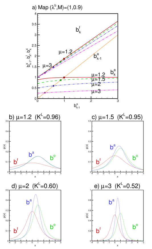
FIG. 4.: a) Graphs of $b_{k}^{\rm f}$ and $b_{k}^{\rm a}$ as function of $b_{k-1}^{\rm a}$ for $(\lambda^{b},M)=(1,0.9)$. For both $b_{k}^{\rm f}$ and $b_{k}^{\rm a}$, the lines represent the corresponding maps and the symbols are the stable fixed-points; solid, dash, dash-dot, and dash-dot-dot lines, as well as circle, square, diamond, and triangle symbols correspond to $\mu=1.2$, 1.5, 2 and 3, respectively; b) error probability distribution for the stable fixed-point corresponding to $\mu=1.2$ and parameters $(x^{\rm f},y^{\rm o})=(0,1)$ and $H=1$, so that $x^{\rm a}=K^{L}$; c, d and e) same as b but corresponding to $\mu=1.5$, 2, and 3, respectively.

FIG. 5.: Stable fixed-point of the Kalman-Lévy filter as a function of $\lambda^{b}$ and $M$: a) $(\bar{b}^{\rm f})^{{1\over\mu}}$, b) $(\bar{b}^{\rm a})^{{1\over\mu}}$ and c) $\bar{K}^{L}$ for $\mu=1.2$; d), e) and f) same as a), b) and c) but for for $\mu=1.5$; g), h) and i) same as a), b) and c) but for for $\mu=2$.

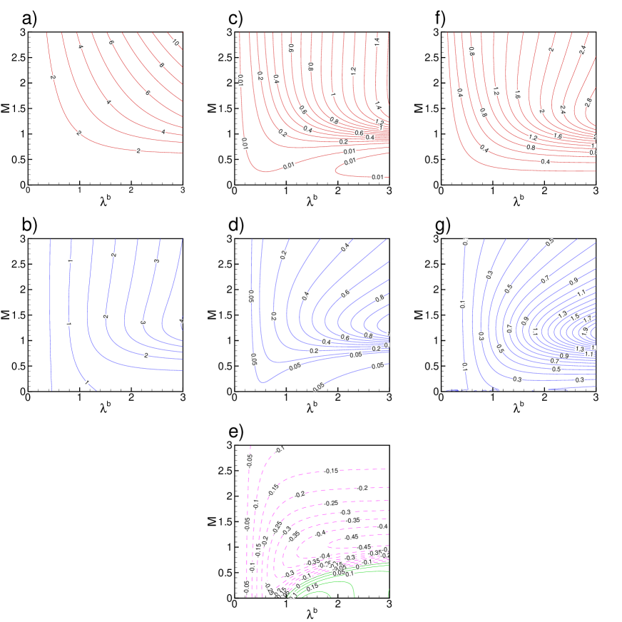
FIG. 6.: Stable fixed-point of the Kalman-Gaussian filter applied to a heavy-tail system with $\mu=1.2$: a) $({\hat{b}}^{\rm f})^{{1\over\mu}}$, b) $({\hat{b}}^{\rm a})^{{1\over\mu}}$, c) difference $({\bar{\hat{b}}}^{\rm f})^{{1\over\mu}}-(\bar{b}^{\rm f})^{{1\over\mu}}$ between the non-optimal filtering solution $({\bar{\hat{b}}}^{\rm f})^{{1\over\mu}}$ shown in a) and the optimal KL filtering solution $(\bar{b}^{\rm f})^{{1\over\mu}}$ shown in Figure 5a, d) difference $({{\hat{b}}}^{\rm a})^{{1\over\mu}}-(\bar{b}^{\rm a})^{{1\over\mu}}$ between the non-optimal filtering solution $({{\hat{b}}}^{\rm a})^{{1\over\mu}}$ shown in b) and the optimal KL filtering solution $(\bar{b}^{\rm a})^{{1\over\mu}}$ shown in Figure 5b, e) difference $K^{G}-K^{L}$ between the non-optimal filtering solution and the model filtering solution. f) difference $({{\hat{b}}}^{\rm f})^{{1\over\mu}}-({\tilde{b}}^{\rm f})^{{1\over{\tilde{\mu}}}}$ between the non-optimal filtering solution $({{\hat{b}}}^{\rm f})^{{1\over\mu}}$ shown in b) and the model filtering solution $({{\tilde{b}}}^{\rm f})^{{1\over{\tilde{\mu}}}}$, g) difference $({{\hat{b}}}^{\rm a})^{{1\over\mu}}-({\tilde{b}}^{\rm a})^{{1\over{\tilde{\mu}}}}$ between the non-optimal filtering solution $({{\hat{b}}}^{\rm a})^{{1\over\mu}}$ shown in b) and the mode filtering solution $({{\tilde{b}}}^{\rm a})^{{1\over{\tilde{\mu}}}}$.

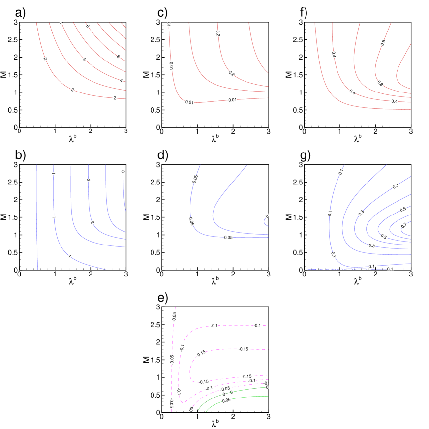
FIG. 7.: Same as figure 6 for dynamical and observational noises given by Lévy distributions with exponent $\mu=1.5$.

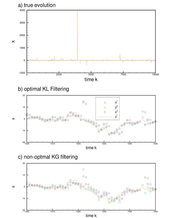
FIG. 8.: Numerical experiment for the parameter set $(\lambda^{b},M)=(1,0.9)$ with $\mu=1.2$; a) evolution of true state variable $x^{\rm t}_{k}$ for $k=1,\ldots,10000$. Note the occurrence of a few large peaks corresponding to rare but extreme noise fluctuations distributed with the Lévy distribution. Panels b) and c) show a magnification of panel a) in the time interval $[1000,1050]$ and compare this true dynamics (continuous line) with the forecasts $x^{f}$ (squares), the observations $y^{o}$ (circles) and the assimilation analysis $x^{a}$ (diamonds). Panel b) corresponds to the use of the optimal KL filtering while panel c) corresponds to the the model filtering with ${\tilde{\mu}}=2$, i.e. standard Kalman-Gaussian filter. It appears clear by visual inspection that the optimal KL analysis $x^{a}$ is much closer more often than not to the true dynamics.

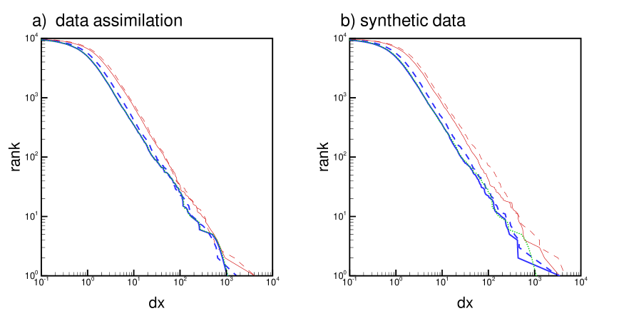
FIG. 9.: a) (Complementary) cumulative distribution (i.e. number of time steps where the error is larger than a value read on the abscissa) of the error between the analysis and the true trajectory for $(\lambda^{b},M)=(1,0.9)$ and $\mu=1.2$, obtained by using the optimal KL filter $K^{L}$ ($x^{\rm a}-x^{\rm t}$; in thick solid line) and model KG filter ${\tilde{K}}_{k}$ (${\tilde{x}}^{\rm a}-x^{\rm t}$; in thick dashed line). We observe clearly that the distribution of $x^{\rm a}-x^{\rm t}$ is below that of ${\tilde{x}}^{\rm a}-x^{\rm t}$, i.e. the errors are globally reduced in distribution by application of the Kalman-Lévy method compared to the standard Kalman-Gaussian method. We also show the cumulative distributions of the difference between forecast and true trajectory for the optimal KL filter $K^{L}$ ($x^{\rm f}-x^{\rm t}$; in solid line) and model KG filter ${\tilde{K}}_{k}$ (${\tilde{x}}^{\rm f}-x^{\rm t}$; in dashed line), as well as the cumulative distributions of the observations ($y^{\rm o}/H-x^{\rm t}$; in dotted line, which is almost identical to $x^{\rm a}-x^{\rm t}$ and thus hardly visible due to the thickness of the lines). b) (Complementary) cumulative distribution of the synthetic simulation of random Lévy variables based on the scale-factors of the stable fixed-points $\bar{b}^{\rm f,a}$ and ${\bar{\hat{b}}}^{\rm f,a}$ (Table I) predicted by the theory. The cumulative distributions of the same observations ($y^{\rm o}/H-x^{\rm t}$; in dotted line) as in a) is also shown for reference. This alternative method for constructive the distributions of errors shows the full consistency of the approach.

REFERENCES

- [1] Abramowitz, E. and Stegun, I.A. (1972) Handbook of mathematical functions. Dover publications, New York.
- [2] Ahn, H. and Feldman, R.E. (1999) Optimal filtering of a Gaussian signal in the presence of Lévy noise, SIAM Journal on Applied Mathematics 60, 359-369.
- [3] Aliev, F.A., and Ozbek, L. (1999) Evaluation of convergence rate in the central limit theorem for the Kalman filter, IEEE Transactions on Automatic Control 44, 1905-1909.
- [4] Bouchaud, J.-P., Sornette, D., Walter C. and Aguilar J.-P. (1998) Taming large events: Optimal portfolio theory for strongly fluctuating assets, International Journal of Theoretical and Applied Finance 1, 25-41.
- [5] Chambers, J.L., C.L. Mallows and B.W. Stuck (1976), A method for simulating stable random variables, Journal of the American Statistical Association 71, 340-344.
- [6] de Calan, C., Luck, J.-M., Nieuwenhuizen, T.M. & Petritis, D., On the distribution of a random variable occurring in 1D disordered systems, J. Phys. A 18, 501-523 (1985).
- [7] Daley, R.A. (1991) Atmospheric data analysis (Cambridge University Press, Cambridge, pp. 457).
- [8] Feller, W. (1966-1971) An introduction to probability theory and its applications, Vol. 2 (New York: J. Wiley and sons).
- [9] Ghil, M. and Malanotte-Rizzoli, P. (1991) Data assimilation in meteorology and oceanography, Adv. Geophys., 33, 141-266.
- [10] Ghil, M., Cohn, S., Travantzis, J., Bube, K. and Isaacson, E. (1981) Application of estimation theory to numerical weather prediction, in Dynamic Meterology, Eds. L Bengtsson, M. Ghil and E. Källén, Springer-Verlag, New York.
- [11] Gnedenko, B.V. and Kolmogorov, A.N. (1954) Limit distributions for sum of independent random variables. Addison Wesley, Reading MA.
- [12] Goldie, C.M. (1991) Implicit renewal theory and tails of solutions of random equations, Ann. Appl. Probab. 1, 126-166.
- [13] Ide, K., Courtier, P., Ghil, M. and Lorenc, A. (1997) Unified notation for data assimilation: Operational, sequential and variational. J. Meteor. Soc. Japan 75, 181-189.
- [14] Johnson, N. L., Kotz, S. and Balakrishnan, N. (1994) Continuous univariate distributions, vol. 2 (Wiley, New York)
- [15] Keller, H.B. (1977) Numerical solution of bifurcation and nonlinear eigenvalue problems, in Application of Bifurcation Theory (ed. P.H. Rabinowitz), Academic Press.
- [16] Kesten, H. (1973) Random difference equations and renewal theory for products of random matrices. Acta Mathematica 131, 207-248.
- [17] Le Breton, A. and Musiela, M. (1993) A generalization of the Kalman filter to models with infinite variance, Stochastic Processes and their applications 47, 75-94.
-
[18]
McCulloch, J. H. (1994)
Numerical Approximation of the Symmetric Stable
Distributions and Densities, Ohio State Univ. Economics Dept.
- [19] Miller, R. N., Ghil, M. and Gauthiez, F. (1994) Advanced data assimilation in strongly nonlinear dynamical systems, J. Atmos. Sci., 1037-1056.
- [20] Montroll, E.W. and West, B.J. (1979) On an enriched collection of stochastic processes, in Fluctuation Phenomena, Eds. E.W. Montroll and J.L. Lebowitz, Elsevier Science Publishers B.V., North Holland, Amsterdam.
- [21] Nishenko, S.P. and Barton, C.C. (1993) Scaling laws for natural disasters: application of fractal statistics to life and economic loss data (abstract), Geol.Soc.Amer., Abstracts with Programs 25, 412.
- [22] Samorodnitsky, G. and Taqqu, M.S. (1994) Stable non-Gaussian random processes: stochastic models with infinite variance. Chapman & Hall, New York.
- [23] Sornette, D. (1998) Linear stochastic dynamics with nonlinear fractal properties, Physica A 250, 295-314.
- [24] Sornette, D. and Cont, R.(1997) Convergent multiplicative processes repelled from zero: power laws and truncated power laws, J. Phys. I France 7, 431-444
- [25] Sornette, D. (2000) Critical Phenomena in Natural Sciences (Chaos, Fractals, Self-organization and Disorder: Concepts and Tools) (Springer Series in Synergetics, Heidelberg).
- [26] Spall, J. C. and Wall, K. D. (1984) Asymptotic distribution theory for the Kalman filter state estimator, Commun. Stat.-Theory and Methods 13, 1981-2003.
- [27] Zajdenweber, D. (1995) Business interruption insurance, a risky business - A study on some Paretian risk phenomena, Fractals 3, 601–608.
- [28] Zajdenweber, D. (1996) Extreme values in business interruption insurance, J. Risk and Insurance 63, 95–110.