Effective Charge and Spin Hamiltonian for the
Quarter-Filled Ladder Compound $\alpha^{\prime}$-NaV₂O₅

Abstract

An effective intra- and inter-ladder charge-spin hamiltonian for the quarter-filled ladder compound $\alpha^{\prime}$-NaV₂O₅ has been derived by using the standard canonical transformation method. In the derivation, it is clear that a finite inter-site Coulomb repulsion is needed to get a meaningful result otherwise the perturbation becomes ill-defined. Various limiting cases depending on the values of the model parameters have been analyzed in detail and the effective exchange couplings are estimated. We find that the effective intra-ladder exchange may become ferromagnetic for the case of zig-zag charge ordering in a purely electronic model.

We estimate the magnitude of the effective inter-rung Coulomb repulsion in a ladder and find it to be about one-order of magnitude too small in order to stabilize charge-ordering.

PACS: 71.10.Fd Lattice Fermion models (Hubbard model etc.), 75.30.Et Exchange and super-exchange interactions, 64.60.-i General studies of phase transitions.

I Introduction

Low-dimensional quantum spin systems have received considerable attention from both theoretical as well as experimental point of view due to their unconventional physical properties. $\alpha^{\prime}$-NaV₂O₅, which was believed to be a low-dimensional inorganic spin-Peierls (SP) compound [2] has recently been under intense investigation. $\alpha^{\prime}$-NaV₂O₅ is an insulator and its magnetic susceptibility data fits very well to the one-dimensional Heisenberg chain model yielding an exchange interaction $J$=440 and 560 K for temperatures below and above the spin-Peierls transition temperature T_SP (T_SP$\approx$ 34 K ) respectively [2, 3]. For T$\leq$ T_SP, an isotropic drop in the susceptibility corresponding to a singlet-triplet gap of $\Delta_{SP}$=85 K has been observed.

Recent X-ray structure data analysis [4, 5] at room temperature disfavours the previously reported non-centrosymmetric structure [6] ($C_{2v}^{7}-P2_{1}mn$ space group) where V⁺⁴ spin-1/2 ions form a one-dimensional Heisenberg chain, running along the crystallographic b-direction, separated by chains of V⁺⁵ spin-zero ions. But the evidence for the centrosymmetric point group [5] ($D_{2h}^{13}-Pmmn$) leads to only one type of V-site with a formal valence +4.5 in this compound. The V-sites then form a quarter-filled ladder, running along the b-axis with the rungs along the crystallographic a-axis. In the quarter-filled scenario, the electron spins are not localized at V-ions rather distributed over a V-O-V molecule which has found support by NMR [7] as well as Raman measurements [8].

The nature of the state below T_SP is presently under intense investigation. Isobe and Ueda [2] originally proposed a usual spin-Peierls scenario but the detection of two inequivalent V-sites in NMR [7] indicates a more complicated scenario and the possibility of charge ordering. Several types of charge ordering, including ’in-line’ [9] and ’zig-zag’ [10, 11, 12] ordering has been proposed, but only the zig-zag type of ordering has been found to be in agreement with neutron scattering [12, 13] and anomalous X-ray scattering [14].

Recent determinations of the low-temperature crystal structure found the space group Fmm2 [15, 16] and proposed the existence of three inequivalent V-ions below T_SP [15, 16, 17]. This scenario was investigated by DMRG (density-matrix renormalization group) and a cluster-operator theory [18] and a strong disagreement with neutron scattering data [13] was found. Ohama et al. recentely observed [19] that the aparent contradiction between cyrstallography (three inequivalent V-ions bewlow T_SP) and NMR (two inequivalent V-ions bewlow T_SP) could be resolved when one considers possible subgroups of the originally proposed space group Fmm2[19].

The crystal structure of $\alpha^{\prime}$-NaV₂O₅ at T$>$T_SP is orthorhombic (a=$11.318\,\mbox{\AA}$, b=$3.611\,\mbox{\AA}$, c=$4.797\,\mbox{\AA}$) and consists of double chains of edge-sharing distorted tetragonal VO₅ pyramids running along the orthorhombic b-axis. These double chains are linked together via common corners of the pyramids and form layers. These are stacked along c-direction with no-direct V-O-V links. The Na atoms are located in between these layers. For the orbitals of the d-electrons at V-sites, those with d_xy symmetry are suggested to be the relevant ones above and below T_SP [5]. Due to the special orbital structure, the hopping amplitudes $t_{a}$ and $t_{b}$ are much larger than the inter-ladder hopping $t_{ab}$, $t_{a}$ and $t_{b}$ being the hopping amplitudes along the rung and the ladder direction respectively ($t_{a}\approx 0.38\,\mbox{eV}$, $t_{b}\approx 0.17\,\mbox{eV}$, $t_{ab}\approx 0.012\,\mbox{eV}$). Since $\alpha^{\prime}$-NaV₂O₅ is an insulator, it has been assumed that the on-site Coulomb repulsion $U$ is sufficiently large in comparision to the hopping amplitudes ($U\approx 2.8\,\mbox{eV}$ from DFT calculation [5]). Moreover, one has to introduce the inter-site Coulomb repulsions, $V_{a}$, $V_{b}$, $V_{ab}$ to obtain the required charge ordering. In fact, it has been shown in a Hartree-Fock calculation [10] that the condition $U>V_{a},V_{b},V_{ab}>t_{a},t_{b},t_{ab}$ must be fulfilled in order to achieve a complete charge ordering. We consider this and other limits in the present paper.

In the present work, we take into account the charge dynamics to obtain an effective low energy hamiltonian for $\alpha^{\prime}$-NaV₂O₅. One starts from a pure electronic hamiltonian, which includes electron hopping in and between the ladders as well as the on-site and inter-site Coulomb interactions. The on-site Coulomb interaction $U$ is taken to be the largest parameter in our calculation. Since $\alpha^{\prime}$-NaV₂O₅ is an insulator and we work at quarter-filling, one can project on a subspace of states which contains one electron per rung. Therefore, it is convenient to use an Ising pseudo-spin variable $\tau^{z}=\pm 1/2$ corresponding to a rung with an electron on the right/left site of the rung. This is in the same spirit of Kugel and Khomskii’s treatment of the orbital degeneracy problem in Jahn-Teller systems [20]. The spin and the pseudo-spin operators can be written as,

$$S^{z}={1\over 2}\sum_{\sigma}\sigma(R_{\sigma}^{\dagger}R_{\sigma}+L_{\sigma}^{\dagger}L_{\sigma}),\;S^{+}=R_{\uparrow}^{\dagger}R_{\downarrow}+L_{\uparrow}^{\dagger}L_{\downarrow},\;S^{-}=R_{\downarrow}^{\dagger}R_{\uparrow}+L_{\downarrow}^{\dagger}L_{\uparrow},\;$$ (1)

$$\tau^{z}={1\over 2}\sum_{\sigma}(R_{\sigma}^{\dagger}R_{\sigma}-L_{\sigma}^{\dagger}L_{\sigma}),\;\tau^{+}=\sum_{\sigma}R_{\sigma}^{\dagger}L_{\sigma},\;\tau^{-}=\sum_{\sigma}L_{\sigma}^{\dagger}R_{\sigma},$$ (2)

which for example yields, $R_{i,\uparrow}^{\dagger}L_{i,\uparrow}=\tau_{i}^{+}({1\over 2}+S_{i}^{z})$,  $R_{i,\uparrow}^{\dagger}L_{i,\downarrow}=\tau_{i}^{+}S_{i}^{+}$,  $L_{i,\downarrow}^{\dagger}L_{i,\uparrow}=({1\over 2}-\tau_{i}^{z})S_{i}^{-}$, etc., where $\tau^{\pm}=\tau^{x}+i\tau^{y}$, $S^{\pm}=S^{x}+iS^{y}$ and $R_{i,\sigma}^{\dagger}(L_{i,\sigma}^{\dagger})$ are the creation operator of an electron with spin $\sigma$ on the right (left) site of the i-th rung of the ladder. In (1) and (2) we have suppressed the site-indices.

II Intra-ladder Exchange

Let us start with an electronic hamiltonian for the quarter-filled ladder (see Fig. 1), which can be written as, $H=H_{0}+H_{0}^{\prime}+H_{I}$, with

$$H_{0}=t_{a}\sum_{i,\sigma}(R_{i,\sigma}^{\dagger}L_{i,\sigma}+h.c.)+U\sum_{i}(n_{i,R\uparrow}n_{i,R,\downarrow}+n_{i,L,\uparrow}n_{i,L,\downarrow})+V_{a}\sum_{i,\sigma,\sigma^{\prime}}n_{i,R,\sigma}n_{i,L,\sigma^{\prime}},$$ (3)

$$H_{0}^{\prime}=V^{\prime}_{b}\sum_{i,\sigma,\sigma^{\prime}}(n_{i,L,\sigma}n_{i+1,L,\sigma^{\prime}}+n_{i,R,\sigma}n_{i+1,R,\sigma^{\prime}})+V^{\prime\prime}_{b}\sum_{i,\sigma,\sigma^{\prime}}(n_{i,L,\sigma}n_{i+1,R,\sigma^{\prime}}+n_{i,R,\sigma}n_{i+1,L,\sigma^{\prime}})$$ (4)

$$+V_{ab}\sum_{<m,n>,\sigma,\sigma^{\prime}}n_{m,R,\sigma}n_{n,L,\sigma^{\prime}},$$ (5)

$$H_{I}=t_{b}\sum_{i,\sigma}(R_{i,\sigma}^{\dagger}R_{i+1,\sigma}+L_{i,\sigma}^{\dagger}L_{i+1,\sigma}+h.c.)+t_{ab}\sum_{<m,n>,\sigma}(R_{m,\sigma}^{\dagger}L_{n,\sigma}+L_{n,\sigma}^{\dagger}R_{m,\sigma}),$$ (6)

where $t_{a}$, $U$ and $V_{a}$ are the hopping integral, on-site and the inter-site Coulomb repulsion in a rung respectively. $t_{b}$, $V^{\prime}_{b}$ and $V^{\prime\prime}_{b}$ are the hopping integral and the Coulomb interaction in between rungs in a ladder, whereas $t_{ab}$ and $V_{ab}$ are the inter-ladder hopping and the Coulomb interaction respectively. $n_{i,R,\sigma}(n_{i,L,\sigma})$ is the electron density operator with spin $\sigma$ in the right (left) site of i-th rung and $<m,n>$ denotes the pair of rungs $m$ and $n$ on adjacent ladders.

We estimate the parameters of the inter-site Coulomb repulsion using a screened Coulomb repulsion, $V=e^{2}/(\epsilon d)$, where $\epsilon$ is the dielectric constant and $d$ the distance between the respective Vanadium atoms. The distance in between two V-ions along the rung and the leg of the ladder (a- and b-directions) are $3.502\,\mbox{\AA}$ and $3.611\,\mbox{\AA}$. The dielectric constant is $\epsilon=11$ from microwave and far infrared measurements [22]. One obtains, $V_{a}=0.3738\,\mbox{eV}$ and $V^{\prime}_{b}=0.3625\,\mbox{eV}$. The diagonal V-V distance in the b-direction in the ladder is $5.030\,\mbox{\AA}$, which implies, $V^{\prime\prime}_{b}=0.2643\,\mbox{eV}$. It will be clear from the later discussion that the effective inter-rung Coulomb repulsion $V_{b}$ is given by the difference between $V^{\prime}_{b}$ and $V^{\prime\prime}_{b}$, i.e. $V_{b}=V^{\prime}_{b}-V^{\prime\prime}_{b}$, which comes out to be small ($V_{b}=0.1023\,\mbox{eV}$) compared to $V_{a}$. Next, $V_{ab}=0.4305\,\mbox{eV}$, as the V-V inter-ladder distance is $3.0401\,\mbox{\AA}$. Note that $V_{ab}$ is slightly higher than $V_{a}$ and nearly four times higher than $V_{b}$.

In order to develop a perturbation expansion, we start by considering the case of a single two-leg quarter-filled ladder. The one-electron eigenstates of $H_{0}$ for a single rung consist of bonding and anti-bonding wave functions, which we denote as $a^{\dagger}|0>={1\over\sqrt{2}}(R^{\dagger}-L^{\dagger})|0>$ and $s^{\dagger}|0>={1\over\sqrt{2}}(R^{\dagger}+L^{\dagger})|0>$, with eigenenergies $-t_{a}$ and $+t_{b}$ respectively. Now let us consider the coupling of the rungs along the legs described by the first term in the hamiltonian $H_{I}$. In order to obtain a coupling between the pseudo-spin and the spin variables, we use here the standard canonical transformation method [21], which is given by,

$$H_{eff}=e^{iS}He^{-iS},$$ (7)

where the operator $S$ is determined from the condition

$$H_{I}+i[S,H_{0}]=0,$$ (8)

which turns out to be

$$\hat{S}=\sum_{n,n^{\prime}}{i\over{(E_{n}^{\prime}-E_{n})}}|n><n|H_{I}|n^{\prime}><n^{\prime}|.$$ (9)

Thus, the effective hamiltonian can be written as,

$$H_{eff}=H_{0}+H^{\prime}_{0}-{1\over 2}\sum_{n,n^{\prime},n^{\prime\prime}}\left({1\over{E_{n}^{\prime}-E_{n}}}+{1\over{E_{n}^{\prime}-E_{n}^{\prime\prime}}}\right)|n><n|H_{I}|n^{\prime}><n^{\prime}|H_{I}|n^{\prime\prime}><n^{\prime\prime}|,$$ (10)

where the initial and the final states $|n^{\prime\prime}>$ and $|n>$ are the two-rung states, i.e., all possible combinations of the bonding and the anti-bonding states between the nearest neighbour rungs. In the present case, there are sixteen possible such states which are the following:

$$s_{i,\sigma}^{\dagger}s_{j,\sigma^{\prime}}^{\dagger}|0>,\;s_{i,\sigma}^{\dagger}a_{j,\sigma^{\prime}}^{\dagger}|0>,\;a_{i,\sigma}^{\dagger}s_{j,\sigma^{\prime}}^{\dagger}|0>,\;a_{i,\sigma}^{\dagger}a_{j,\sigma^{\prime}}^{\dagger}|0>,$$ (11)

with $\sigma,\sigma^{\prime}=\uparrow,\downarrow$. The six intermediate states $|n^{\prime}>$ which are the two-particle excited states in a rung, have to be antisymmetric under the exchange of both spin and pseudo-spin coordinates, in accordance with the Pauli principle. Thus, we have two sectors for the excited states depending on the total and the z-component of spin as well as the pseudo-spin quantum numbers which are labeled as, $|S,S^{z};\tau,\tau^{z}>$. Hence, the states involved are, $|0,0;1,1>=R_{i,\uparrow}^{\dagger}R_{i,\downarrow}^{\dagger}|0>$,  $|0,0;1,-1>=L_{i,\uparrow}^{\dagger}L_{i,\downarrow}^{\dagger}|0>$,  $|0,0;1,0>={1\over\sqrt{2}}(R_{i,\uparrow}^{\dagger}L_{i,\downarrow}^{\dagger}-R_{i,\downarrow}^{\dagger}L_{i,\uparrow}^{\dagger})|0>$   and   $|1,1;0,0>=R_{i,\uparrow}^{\dagger}L_{i,\uparrow}^{\dagger}|0>$,   $|1,-1;0,0>=R_{i,\downarrow}^{\dagger}L_{i,\downarrow}^{\dagger}|0>$,  $|1,0;0,0>={1\over\sqrt{2}}(R_{i,\uparrow}^{\dagger}L_{i,\downarrow}^{\dagger}+R_{i,\downarrow}^{\dagger}L_{i,\uparrow}^{\dagger})|0>$. The eigenenergies of the excited states in the large $U$ limit are $V_{a}$ for the spin-triplet states $|1,S^{z};0,0>$ ($S^{z}=-1,0+1$). For the spin-singlets, the eigenenergies are $U^{\prime}$ for ${1\over\sqrt{2}}(|0,0;1,1>+|0,0;1,-1>)$ (symmetric), $U$ for ${1\over\sqrt{2}}(|0,0;1,1>-|0,0;1,-1>)$ (antisymmetric) and $V^{\prime}_{a}$ for $|0,0;1,0>$, with $U^{\prime}\approx U+{{4t_{a}^{2}}\over{U-V_{a}}}$ and $V^{\prime}_{a}\approx V_{a}-{{4t_{a}^{2}}\over{U-V_{a}}}$. After some lengthy but straightforward algebra and in the case of large but finite $U$, the total effective hamiltonian can be written as,

$$H_{eff}=H_{0}+H^{\prime}_{0}+H_{eff}^{intra}+H_{eff}^{inter},$$ (12)

where $H_{eff}^{intra}$ is the effective intra-ladder hamiltonian which one can express as, $H_{eff}^{intra}=H_{eff}^{(t)}+H_{eff}^{(s)}$, with $H_{eff}^{(t)}$ and $H_{eff}^{(s)}$ being the contribution due to the intermediate spin-triplet and spin-singlet states respectively. $H_{eff}^{inter}$ is the effective inter-ladder hamiltonian which can be derived in a similar way and will be discussed in the next section. In terms of the pseudo-spin and spin variables, the unperturbed hamiltonian $H_{0}$ and $H^{\prime}_{0}$ can be expressed as,

$$H_{0}=2t_{a}\sum_{i}\tau_{i}^{x},$$ (13)

$$H^{\prime}_{0}=2(V^{\prime}_{b}-V^{\prime\prime}_{b})\sum_{i}\left({1\over 4}+\tau_{i}^{z}\tau_{i+1}^{z}\right)\,+\,N\,V_{b}^{\prime\prime}+V_{ab}\sum_{<m,n>}\left({1\over 4}-\tau_{m}^{z}\tau_{n}^{z}+{{\tau_{m}^{z}-\tau_{n}^{z}}\over 2}\right),$$ (14)

where $N$ is the number of rungs. In a similar way, the effective hamiltonian $H_{eff}^{(t)}$ can be written as,

$$H_{eff}^{(t)}=-{{4t_{b}^{2}}\over{V_{a}}}\sum_{i}\left({1\over 4}-\vec{\tau}_{i}\cdot\vec{\tau}_{i+1}\right)\left({3\over 4}+\vec{S}_{i}\cdot\vec{S}_{i+1}\right).$$ (15)

It is obvious from the above expression that $H_{eff}^{(t)}$ is independent of the Coulomb correlation energy $U$. This is due to the fact that while deriving this effective hamiltonian we have used the eigenenergies for the excited states which happen to be $V_{a}$ for this case. Since the effective hamiltonian $H_{eff}^{(s)}$ is obtained due to the contribution from the same intermediate states $|n^{\prime}>$ and different initial and final states $|n>$ and $|n^{\prime\prime}>$, it can be written as, $H_{eff}^{(s)}=H_{eff}^{(s1)}+H_{eff}^{(s2)}+H_{eff}^{(s3)}$ (which are the contributions due to the antisymmetric, symmetric and $|0,0;1,0>$ intermediate states), with

$$H_{eff}^{(s1)}=-{{4t_{b}^{2}}\over{U}}\sum_{i}\left({1\over 4}-2\tau_{i}^{x}\tau_{i+1}^{x}+\vec{\tau}_{i}\cdot\vec{\tau}_{i+1}\right)\left({1\over 4}-\vec{S}_{i}\cdot\vec{S}_{i+1}\right),$$ (16)

$$H_{eff}^{(s2)}=-{{2t_{b}^{2}}\over{U^{\prime}-2t_{a}}}\sum_{i}\left({1\over 4}+{{\tau_{i}^{x}+\tau_{i+1}^{x}}\over{2}}-2\tau_{i}^{y}\tau_{i+1}^{y}+\vec{\tau}_{i}\cdot\vec{\tau}_{i+1}\right)\left({1\over 4}-\vec{S}_{i}\cdot\vec{S}_{i+1}\right)$$ (17)

$$-{{2t_{b}^{2}}\over{U^{\prime}+2t_{a}}}\sum_{i}\left({1\over 4}-{{\tau_{i}^{x}+\tau_{i+1}^{x}}\over{2}}-2\tau_{i}^{y}\tau_{i+1}^{y}+\vec{\tau}_{i}\cdot\vec{\tau}_{i+1}\right)\left({1\over 4}-\vec{S}_{i}\cdot\vec{S}_{i+1}\right),$$ (18)

$$H_{eff}^{(s3)}=-{{2t_{b}^{2}}\over{V^{\prime}_{a}-2t_{a}}}\sum_{i}\left({1\over 4}+{{\tau_{i}^{x}+\tau_{i+1}^{x}}\over{2}}-2\tau_{i}^{z}\tau_{i+1}^{z}+\vec{\tau}_{i}\cdot\vec{\tau}_{i+1}\right)\left({1\over 4}-\vec{S}_{i}\cdot\vec{S}_{i+1}\right)$$ (19)

$$-{{2t_{b}^{2}}\over{V^{\prime}_{a}+2t_{a}}}\sum_{i}\left({1\over 4}-{{\tau_{i}^{x}+\tau_{i+1}^{x}}\over{2}}-2\tau_{i}^{z}\tau_{i+1}^{z}+\vec{\tau}_{i}\cdot\vec{\tau}_{i+1}\right)\left({1\over 4}-\vec{S}_{i}\cdot\vec{S}_{i+1}\right).$$ (20)

It should be noted here that one gets a non-zero contribution to $H_{eff}^{(t)}$ and $H_{eff}^{(s)}$ even if $U=\infty$ which will be discussed below. Moreover, it is obvious from the expression for $H_{eff}^{(t)}$ (see Eq. (15)) that a finite $V_{a}$ is indeed needed to get a meaningful result otherwise the perturbation becomes ill-defined for $V_{a}=0$.

Limiting Cases and Discussion

Case I: $t_{a}=0$: This limit implies $U^{\prime}=U$ and $V^{\prime}_{a}=V_{a}$ and thus, $H_{eff}^{(s1)}$ and $H_{eff}^{(s2)}$ can be combined together to yield,

$$H_{eff}^{(s1)}+H_{eff}^{(s2)}=-{{8t_{b}^{2}}\over{U}}\sum_{i}\left({1\over 4}+\tau_{i}^{z}\tau_{i+1}^{z}\right)\left({1\over 4}-\vec{S}_{i}\cdot\vec{S}_{i+1}\right),$$ (21)

whereas the effective hamiltonian $H_{eff}^{(s3)}$ gets reduced to,

$$H_{eff}^{(s3)}=-{{4t_{b}^{2}}\over{V_{a}}}\sum_{i}\left({1\over 4}+\vec{\tau}_{i}\cdot\vec{\tau}_{i+1}-2\tau_{i}^{z}\tau_{i+1}^{z}\right)\left({1\over 4}-\vec{S}_{i}\cdot\vec{S}_{i+1}\right).$$ (22)

Since $H_{eff}^{(t)}$ neither depends on $t_{a}$ nor on $U$, it doesn’t get affected in the above limiting case and the same is true for the other cases considered below. The effective hamiltonian derived by Thalmeier and Fulde [9] corresponds to Eq. (21).

Case II: $t_{a}=0$, $U=\infty$: In this limit, which also corresponds to the limit $V_{a}\gg 2t_{a}$, the contribution to the effective hamiltonian from $H_{eff}^{(s1)}$ and $H_{eff}^{(s2)}$ vanish and thus, the total intra-ladder effective hamiltonian becomes the sum of $H_{eff}^{(t)}$ and $H_{eff}^{(s3)}$ (see Eq. (15) and (22)). This is what is exactly obtained by Mostovoy and Khomskii [11] but with a different interpretation.

Case III: $U=\infty$, $V_{a}\ll 2t_{a}$: In this case, the effective hamiltonian $H_{eff}^{(s1)}$ and $H_{eff}^{(s2)}$ vanish but $H_{eff}^{(s3)}$ reduces to,

$$H_{eff}^{(s3)}={{t_{b}^{2}}\over{t_{a}}}\sum_{i}\left(\tau_{i}^{x}+\tau_{i+1}^{x}\right)\left({1\over 4}-\vec{S}_{i}\cdot\vec{S}_{i+1}\right),$$ (23)

so that the total effective intra-ladder hamiltonian becomes the sum of Eq. (15) and (23). Moreover, since $V_{a}\ll 2t_{a}$, the major contribution will be from Eq. (15).

Case IV: Disordered Phase: In the disordered phase, where the electrons are in the bonding states (see Fig. 2 (a)), we can get an estimate of the effective exchange coupling in the effective hamiltonian by taking the averages over its charge (pseudo-spin) part. One can write down the effective exchange hamiltonian (disregarding the constant factors) as, $H_{eff}^{exch}=J_{eff}^{exch}\sum_{i}\vec{S}_{i}\cdot\vec{S}_{i+1}$. In the present case, we have, $<\tau_{i}^{x}>=-1/2$ and $<\tau_{i}^{y}>=0=<\tau_{i}^{z}>$ whereas $<\tau_{i}^{x}\tau_{i+1}^{x}>=1/4$ and $<\tau_{i}^{y}\tau_{i+1}^{y}>=0=<\tau_{i}^{z}\tau_{i+1}^{z}>$. Thus, the effective exchange coupling due to the hamiltonian $H_{eff}^{(t)}$ and $H_{eff}^{(s1)}$ vanish, but that of $H_{eff}^{(s2)}$ and $H_{eff}^{(s3)}$ become, ${{-2t_{b}^{2}}\over{U^{\prime}+2t_{a}}}$ and ${{-2t_{b}^{2}}\over{V^{\prime}_{a}+2t_{a}}}$ which yields $J_{eff}^{exch}={2t_{b}^{2}}({1\over{U^{\prime}+2t_{a}}}+{1\over{V^{\prime}_{a}+2t_{a}}})$. It is clear that the exchange coupling here is antiferromagnetic ($>0$). Using the parameters mentioned in the present work, $J_{eff}^{exch}$ is estimated to be 0.08 eV. The expression for $J_{eff}^{exch}$ is exactly the same (for the case $V_{a}=0$) as obtained by Horsch and Mack [23].

Case V: Complete Charge Ordered Phase: We can get an estimate of the effective exchange couplings in the completely charge ordered (zig-zag) phase (see Fig. 2 (b, c)), following the same procedure as that of the disordered phase. Here, one has, $<\tau_{i}^{x}>=0=<\tau_{i}^{y}>$ and $<\tau_{i}^{z}>=1/2$,  $<\tau_{i+1}^{z}>=-1/2$ whereas $<\tau_{i}^{x}\tau_{i+1}^{x}>=0=<\tau_{i}^{y}\tau_{i+1}^{y}>$ and $<\tau_{i}^{z}\tau_{i+1}^{z}>=-1/4$. Hence, the effective exchange coupling due to $H_{eff}^{(s1)}$ and $H_{eff}^{(s2)}$ vanish but that of $H_{eff}^{(t)}$ and $H_{eff}^{(s3)}$ survive, which ultimately leads to $J_{eff}^{exch}={-2t_{b}^{2}}[{1\over{V_{a}}}-{1\over{2(V^{\prime}_{a}-2t_{a})}}-{1\over{2(V^{\prime}_{a}+2t_{a})}}]$. However, using the parameter values, it is calculated to be -0.17 eV. In the case where $U=\infty$ and for $0<(V_{a}/2t_{a})<1$, $J_{eff}^{exch}$ becomes ferromagnetic ($<0$) whereas for $(V_{a}/2t_{a})>1$, it is antiferromagnetic. The variation of $J_{eff}^{exch}$ with respect to the parameter $(V_{a}/2t_{a})$ is shown in Fig. 4. It is clear from the figure that there exists a minimum in the ferromagnetic region for $(V_{a}/2t_{a})=1/\sqrt{3}$, where $J_{eff}^{exch,min}=-2.26\,({{t_{b}^{2}}/t_{a}})=-0.2\,\mbox{eV}$, which is quite large.

III Inter-ladder Exchange

Next, let us consider the hopping between the two nearest neighbour ladders, which is described by the second term of the hamiltonian $H_{I}$ (see Eq. (6)), i.e.,

$$H_{I}^{inter}=t_{ab}\sum_{<m,n>,\sigma}(R_{m,\sigma}^{\dagger}L_{n,\sigma}+L_{n,\sigma}^{\dagger}R_{m,\sigma}).$$ (24)

The effective inter-ladder coupling between the charge and the spin degrees of freedom is derived in the same way as has been done for the single ladder case. Since the two-particle excited states in this case are exactly the same as what has been done earlier, the effective inter-ladder hamiltonian can be written as sum of two parts, i.e., $H_{eff}^{inter}=H_{eff}^{inter(t)}+H_{eff}^{inter(s)}$, where the superscript ‘$t$’ and ‘$s$’ have the same meaning discussed in the previous section. The effective hamiltonian $H_{eff}^{inter(t)}$ is derived to be,

$$H_{eff}^{inter(t)}=-{{t_{ab}^{2}}\over{2(V_{a}-2t_{a})}}\sum_{<m,n>}\left({1\over 4}+{{\tau_{m}^{x}+\tau_{n}^{x}}\over{2}}-2\tau_{m}^{y}\tau_{n}^{y}+\vec{\tau}_{m}\cdot\vec{\tau}_{n}\right)\left({3\over 4}+\vec{S}_{m}\cdot\vec{S}_{n}\right)$$ (25)

$$-{{t_{ab}^{2}}\over{2(V_{a}+2t_{a})}}\sum_{<m,n>}\left({1\over 4}-{{\tau_{m}^{x}+\tau_{n}^{x}}\over{2}}-2\tau_{m}^{y}\tau_{n}^{y}+\vec{\tau}_{m}\cdot\vec{\tau}_{n}\right)\left({3\over 4}+\vec{S}_{m}\cdot\vec{S}_{n}\right)$$ (26)

$$-{{t_{ab}^{2}}\over{V_{a}}}\sum_{<m,n>}\left({1\over 4}-2\tau_{m}^{x}\tau_{n}^{x}+\vec{\tau}_{m}\cdot\vec{\tau}_{n}\right)\left({3\over 4}+\vec{S}_{m}\cdot\vec{S}_{n}\right),$$ (27)

whereas $H_{eff}^{inter(s)}$ can be written as $H_{eff}^{inter(s)}=H_{eff}^{inter(s1)}+H_{eff}^{inter(s2)}+H_{eff}^{inter(s3)}$, with

$$H_{eff}^{inter(s1)}={-{t_{ab}^{2}}\over{2(U-2t_{a})}}\sum_{<m,n>}$$ (28)

$$\left({1\over 4}+{{\tau_{m}^{x}+\tau_{n}^{x}}\over{2}}+{{\tau_{m}^{z}-\tau_{n}^{z}}\over{2}}-2\tau_{m}^{z}\tau_{n}^{z}-\tau_{m}^{x}\tau_{n}^{z}+\tau_{m}^{z}\tau_{n}^{x}+\vec{\tau}_{m}\cdot\vec{\tau}_{n}\right)\left({1\over 4}-\vec{S}_{m}\cdot\vec{S}_{n}\right)$$ (29)

$$-{{t_{ab}^{2}}\over{2(U+2t_{a})}}\sum_{<m,n>}$$ (30)

$$\left({1\over 4}-{{\tau_{m}^{x}+\tau_{n}^{x}}\over{2}}+{{\tau_{m}^{z}-\tau_{n}^{z}}\over{2}}-2\tau_{m}^{z}\tau_{n}^{z}+\tau_{m}^{x}\tau_{n}^{z}-\tau_{m}^{z}\tau_{n}^{x}+\vec{\tau}_{m}\cdot\vec{\tau}_{n}\right)\left({1\over 4}-\vec{S}_{m}\cdot\vec{S}_{n}\right)$$ (31)

$$-{{t_{ab}^{2}}\over{U}}\sum_{<m,n>}\left({1\over 4}+{{\tau_{m}^{z}-\tau_{n}^{z}}\over{2}}-\vec{\tau}_{m}\cdot\vec{\tau}_{n}\right)\left({1\over 4}-\vec{S}_{m}\cdot\vec{S}_{n}\right).$$ (32)

The expression for $H_{eff}^{inter(s2)}$ is exactly the same as that of $H_{eff}^{inter(s1)}$ except that $U$ here is replaced by $U^{\prime}$. On the other hand, $H_{eff}^{inter(s3)}$ is obtained as,

$$H_{eff}^{inter(s3)}=-{{t_{ab}^{2}}\over{2(V^{\prime}_{a}-2t_{a})}}\sum_{<m,n>}\left({1\over 4}+{{\tau_{m}^{x}+\tau_{n}^{x}}\over{2}}-2\tau_{m}^{y}\tau_{n}^{y}+\vec{\tau}_{m}\cdot\vec{\tau}_{n}\right)\left({1\over 4}-\vec{S}_{m}\cdot\vec{S}_{n}\right)$$ (33)

$$-{{t_{ab}^{2}}\over{2(V^{\prime}_{a}+2t_{a})}}\sum_{<m,n>}\left({1\over 4}-{{\tau_{m}^{x}+\tau_{n}^{x}}\over{2}}-2\tau_{m}^{y}\tau_{n}^{y}+\vec{\tau}_{m}\cdot\vec{\tau}_{n}\right)\left({1\over 4}-\vec{S}_{m}\cdot\vec{S}_{n}\right)$$ (34)

$$-{{t_{ab}^{2}}\over{V^{\prime}_{a}}}\sum_{<m,n>}\left({1\over 4}-2\tau_{m}^{x}\tau_{n}^{x}+\vec{\tau}_{m}\cdot\vec{\tau}_{n}\right)\left({1\over 4}-\vec{S}_{m}\cdot\vec{S}_{n}\right).$$ (35)

Since the derivation of the effective inter-ladder hamiltonian proceeds in the same way as that of the intra-ladder case, the limiting cases will follow the same way as has been done before. Moreover, here also, one needs a finite $V_{a}$ (but $V_{a}\neq 2t_{a}$) in deriving the effective hamiltonian, otherwise the perturbation becomes ill-defined for $V_{a}=0$. Furthermore, one gets a non-zero contribution to the effective inter-ladder hamiltonian even if $U=\infty$ .

Limiting Cases and Discussion

Case I: $t_{a}=0$: In this limit $U^{\prime}=U$ and $V^{\prime}_{a}=V_{a}$ follow naturally. Thus, $H_{eff}^{inter(t)}$ reduces to,

$$H_{eff}^{inter(t)}=-{{2t_{ab}^{2}}\over{V_{a}}}\sum_{<m,n>}\left({1\over 4}+\tau_{m}^{z}\tau_{n}^{z}\right)\left({3\over 4}+\vec{S}_{m}\cdot\vec{S}_{n}\right).$$ (36)

Similarly, $H_{eff}^{inter(s1)}$, $H_{eff}^{inter(s2)}$ and $H_{eff}^{inter(s3)}$ become,

$$H_{eff}^{inter(s1)}+H_{eff}^{inter(s2)}=-{{4t_{ab}^{2}}\over{U}}\sum_{<m,n>}\left({1\over 4}+{{\tau_{m}^{z}-\tau_{n}^{z}}\over{2}}-\tau_{m}^{z}\tau_{n}^{z}\right)\left({1\over 4}-\vec{S}_{m}\cdot\vec{S}_{n}\right),$$ (37)

$$H_{eff}^{inter(s3)}=-{{2t_{ab}^{2}}\over{V_{a}}}\sum_{<m,n>}\left({1\over 4}+\tau_{m}^{z}\tau_{n}^{z}\right)\left(1/4-\vec{S}_{m}\cdot\vec{S}_{n}\right).$$ (38)

The expression Eq. (37) is the same one as has been obtained by Thalmeier and Fulde [9].

Case II: $t_{a}=0$, $U=\infty$: In this case, the contributions from $H_{eff}^{inter(s1)}$and $H_{eff}^{inter(s2)}$ vanish. The contributions from $H_{eff}^{inter(t)}$ and $H_{eff}^{inter(s3)}$ can be combined together to yield,

$$H_{eff}^{inter}=H_{eff}^{inter(t)}+H_{eff}^{inter(s)}=-{{2t_{ab}^{2}}\over{V_{a}}}\sum_{<m,n>}\left({1\over 4}+\tau_{m}^{z}\tau_{n}^{z}\right),$$ (39)

which becomes independent of the spin degrees of freedom.

Case III: $U=\infty$, $V_{a}\ll 2t_{a}$: In this case, the contributions from $H_{eff}^{inter(s1)}$ and $H_{eff}^{inter(s2)}$ vanish. Combining $H_{eff}^{inter(t)}$ and $H_{eff}^{inter(s3)}$, the spin-dependence drops out and one obtains,

$$H_{eff}^{inter}=H_{eff}^{inter(t)}+H_{eff}^{inter(s3)}={{t_{ab}^{2}}\over{4t_{a}}}\sum_{<m,n>}\left(\tau_{m}^{x}+\tau_{n}^{x}\right)-{{t_{ab}^{2}}\over{V_{a}}}\sum_{<m,n>}\left({1\over 4}-2\tau_{m}^{x}\tau_{n}^{x}+\vec{\tau}_{m}\cdot\vec{\tau}_{n}\right).$$ (40)

Case IV: Disordered Phase: Following the procedure already mentioned for the intra-ladder case, we can get an estimate of the effective exchange coupling between the nearest neighbour ladders (see Fig. 3 (a)) by taking the averages over the charge part in the effective hamiltonian. Here also, one can write down the effective hamiltonian (disregarding the constant factors) as, $H_{eff}^{inter,exch}=(J_{eff}^{inter,exch(t)}+J_{eff}^{inter,exch(s)})\sum_{<m,n>}\vec{S}_{m}\cdot\vec{S}_{n}=J_{eff}^{inter,exch}\sum_{<m,n>}\vec{S}_{m}\cdot\vec{S}_{n}$. In the present case, one has, $<\tau_{m}^{x}>=<\tau_{n}^{x}>=-1/2$ and $<\tau_{m}^{y}>=<\tau_{n}^{y}>=0=<\tau_{m}^{z}>=<\tau_{n}^{z}>$ whereas $<\tau_{m}^{x}\tau_{n}^{x}>=1/4$ and $<\tau_{m}^{y}\tau_{n}^{y}>=0=<\tau_{m}^{z}\tau_{n}^{z}>$. Thus, the effective exchange coupling which is due to $H_{eff}^{inter(t)}$, $H_{eff}^{inter(s1)}$, $H_{eff}^{inter(s2)}$ and $H_{eff}^{inter(s3)}$ is given as, $J_{eff}^{inter,exch}={{-t_{ab}^{2}}\over{2}}[{1\over{(V_{a}+2t_{a})}}-{1\over{(U+2t_{a})}}-{1\over{(U^{\prime}+2t_{a})}}-{1\over{(V^{\prime}_{a}+2t_{a})}}]$. The exchange coupling here is antiferromagnetic and is estimated to be $(J_{eff}^{inter,exch}/t_{ab}^{2})=0.39$. For $V_{a}=0$, it gives rise to the same expression as obtained by Horsch and Mack [23].

Case V: Complete Charge Ordered Phase: Here, we have four different completely charge ordered (zig-zag) phase depending on the state through which we compute the averages over the charge part of the effective hamiltonian. In all these cases, one has, $<\tau_{m}^{x}>=<\tau_{n}^{x}>=0=<\tau_{m}^{y}>=<\tau_{n}^{y}>$ and $<\tau_{m}^{x}\tau_{n}^{x}>=0=<\tau_{m}^{y}\tau_{n}^{y}>$. In addition to this, one has,

  (i)

$<\tau_{m}^{z}>=1/2$, $<\tau_{n}^{z}>=-1/2$ and $<\tau_{m}^{z}\tau_{n}^{z}>=-1/4$, where the averages are due to the state $R_{m,\alpha}^{\dagger}L_{n,\beta}^{\dagger}|0>$ (Fig. 3 (b)). The effective exchange coupling for $H_{eff}^{inter(t)}$ and $H_{eff}^{inter(s3)}$ vanish but that of $H_{eff}^{inter(s1)}$ and $H_{eff}^{inter(s2)}$ are finite which gives rise to, $J_{eff}^{inter,exch}={t_{ab}^{2}}[{1\over{2(U-2t_{a})}}+{1\over{2(U+2t_{a})}}+{1\over{U}}+{1\over{2(U^{\prime}-2t_{a})}}+{1\over{2(U^{\prime}+2t_{a})}}+{1\over{U^{\prime}}}]$. The exchange coupling here is antiferromagnetic and is estimated to be $(J_{eff}^{inter,exch}/t_{ab}^{2})=1.42$. For $t_{a}=0$, it gives rise to usual super-exchange, i.e. $J_{eff}^{inter,exch}={{4t_{ab}^{2}}/U}$.

  (ii)

$<\tau_{m}^{z}>=-1/2$, $<\tau_{n}^{z}>=1/2$, and $<\tau_{m}^{z}\tau_{n}^{z}>=-1/4$, where the averages are taken over the state $L_{m,\alpha}^{\dagger}R_{n,\beta}^{\dagger}|0>$ (Fig. 3 (c)). In this case, $J_{eff}^{inter,exch(t)}=0=J_{eff}^{inter,exch(s)}$ which ultimately corresponds to the case $J_{eff}^{inter,exch}=0$.

  (iii)

$<\tau_{m}^{z}>=<\tau_{n}^{z}>=1/2$ and $<\tau_{m}^{z}\tau_{n}^{z}>=1/4$, where the averages here are due to the state $R_{m,\alpha}^{\dagger}R_{n,\beta}^{\dagger}|0>$ (Fig. 3 (d)). The effective exchange couplings for $H_{eff}^{inter(s1)}$ and $H_{eff}^{inter(s2)}$ vanish. Thus, $J_{eff}^{inter,exch}$ is obtained from the contribution due to $H_{eff}^{inter(t)}$ and $H_{eff}^{inter(s3)}$ which is, $J_{eff}^{inter,exch}={-t_{ab}^{2}\over 2}[{1\over{2(V_{a}-2t_{a})}}+{1\over{2(V_{a}+2t_{a})}}+{1\over{V_{a}}}-{1\over{2(V^{\prime}_{a}-2t_{a})}}-{1\over{2(V^{\prime}_{a}+2t_{a})}}-{1\over{V^{\prime}_{a}}}]$. The exchange coupling here is antiferromagnetic and is estimated to be $(J_{eff}^{inter,exch}/t_{ab}^{2})=2.8$. It vanishes for $U=\infty$ as well as for $t_{a}=0$.

  (iv)

$<\tau_{m}^{z}>=<\tau_{n}^{z}>=-1/2$ and $<\tau_{m}^{z}\tau_{n}^{z}>=1/4$, where the averages are taken over the state $L_{m,\alpha}^{\dagger}L_{n,\beta}^{\dagger}|0>$ (Fig. 3 (e)). Here, the effective exchange coupling turns out to be the same as that of (iii).

Case VI: A Phase with one Ladder Completely Charge Ordered and the Nearest Neighbour Disordered: In this case, we have two possibilities, again depending on the state through which one computes the averages over the charge part in the effective hamiltonian. In both the cases, one has, $<\tau_{m}^{x}>=0=<\tau_{m}^{y}>$, $<\tau_{n}^{y}>=0=<\tau_{n}^{z}>$ and $<\tau_{m}^{x}\tau_{n}^{x}>=0=<\tau_{m}^{y}\tau_{n}^{y}>=<\tau_{m}^{z}\tau_{n}^{z}>$. Besides, one has,

  (i)

$<\tau_{m}^{z}>=1/2$, $<\tau_{n}^{x}>=-1/2$ and $<\tau_{m}^{z}\tau_{n}^{x}>=-1/4$, where the averages are taken over the state $R_{m,\alpha}^{\dagger}a_{n,\beta}^{\dagger}|0>$ (Fig. 3 (f)). All the effective exchange couplings in this case turn out to be non-zero and hence $J_{eff}^{inter,exch}$ is obtained as, $J_{eff}^{inter,exch}={-t_{ab}^{2}\over 2}{[{1\over{2(V_{a}+2t_{a})}}+{1\over{2V_{a}}}-{1\over{(U+2t_{a})}}-{1\over{U}}-{1\over{(U^{\prime}+2t_{a})}}-{1\over{U^{\prime}}}-{1\over{2(V^{\prime}_{a}+2t_{a})}}-{1\over{2V^{\prime}_{a}}}]}$.

  (ii)

$<\tau_{m}^{z}>=-1/2$, $<\tau_{n}^{x}>=-1/2$ and $<\tau_{m}^{z}\tau_{n}^{x}>=1/4$ where the averages are due to the state $L_{m,\alpha}^{\dagger}a_{n,\beta}^{\dagger}|0>$ (Fig. 3 (g)). The effective exchange coupling which is due to $H_{eff}^{inter(t)}$ and $H_{eff}^{inter(s3)}$ (the contributions due to $H_{eff}^{inter(s1)}$ and $H_{eff}^{inter(s2)}$ vanish) is given by, $J_{eff}^{inter,exch}={-t_{ab}^{2}\over 2}{[{1\over{2(V_{a}+2t_{a})}}+{1\over{2V_{a}}}-{1\over{2(V^{\prime}_{a}+2t_{a})}}-{1\over{2V^{\prime}_{a}}}]}$.

In both of the above mentioned cases, the exchange coupling becomes antiferromagnetic and is estimated to be $(J_{eff}^{inter,exch}/t_{ab}^{2})=2.26$ for case (i) and 1.65 for (ii). However, it vanishes in both cases for $U=\infty$ irrespective of whether $V_{a}\gg 2t_{a}$ or $V_{a}\ll 2t_{a}$.

IV Discussion and Conclusion

We have derived the effective spin-charge hamiltonian for $\alpha^{\prime}$-NaV₂O₅ for both intra-ladder and inter-ladder exchange. We find a rich structure as a function of possible realization of the microscopic parameters. We have found several, in part unexpected, results.

  (i)

The effective magnetic exchange along the ladder decreases with increasing charge ordering (of zig-zag type). For complete charge ordering, the magnetic exchange becomes ferromagnetic and quite large in magnitude.

  (ii)

The effective inter-ladder magnetic exchange in between two given rungs of a charge-ordered and a charge-disordered ladder changes (only) by a factor of two when the charge-density-wave is shifted by a lattice constant along $a$ (compare Fig. 3 (f) and (g)).

  (iii)

There are novel terms of type $\tau_{m}^{z}\tau_{n}^{x}$ in the effective charge-charge inter-ladder interaction. These terms, which are however rather small in magnitude, could in principle stabilize a mixed charge-order configurations like the one illustrated in Fig. 3 (f) and (g).

As a consequence of (i) and (ii), the proposed frustrated spin-cluster model by de Boer et al. [16] seems to be unlikely, since (a) no indications of ferromagnetic couplings have been found experimentally and (b) the coupling in between the one-dimensional spin-cluster chains of Ref. [16] should be, as a consequence of (ii), rather strong. This conclusion is consistent with a recent study of the frustrated spin-cluster model by DMRG and a cluster-operator theory [18].

Let us note that the change in sign of the effective intra-ladder magnetic exhange shown in Fig. 4 cannot be described accurately by a perturbation expansion in $t_{b}$. Near to the singularity at $V_{a}=2t_{a}$ the perturbation expansion breaks down and the effective intra-ladder spin-hamiltonian becomes long-ranged.

Ultimately, the reason for the ferromagnetic intra-ladder coupling for the zig-zag ordering found in the above calculation lies in the fact that the charge-ordered state is not the ground-state of $H_{0}$. In fact, the charge-ordered state would be stabilized by $H_{0}^{\prime}$ in the case of a large effective inter-rung Coulomb-coupling $V_{b}^{\prime}-V_{b}^{\prime\prime}$ (see Eq. (14)). For large values of $V_{b}^{\prime}-V_{b}^{\prime\prime}\gg 2t_{a}$, the perturbation expansion would yield (e.g. in mean-field approximation for $H_{0}^{\prime}$) an antiferromagnetic intra-ladder spin-spin coupling. We did not show this calculation here, since our estimated value for the inter-rung Coulomb repulsion $V_{b}^{\prime}-V_{b}^{\prime\prime}\approx 0.1\,\mbox{eV}$ is about one-order of magnitude too small in order to do the job. We therefore believe that this small value of $V_{b}^{\prime}-V_{b}^{\prime\prime}$ indicates (a) the importance of elastic effects for the stabilization of the observed phase transition at $T_{c}=34\,\mbox{K}$ and (b) that the degree of charge ordering is far from complete. This is consistent with the proposal of about 20% charge ordering [12].

FIG. 1.: Schematic structure of $\alpha^{\prime}$-NaV₂O₅ where the open circles stands for the Vanadium sites. Different parameters are also shown.

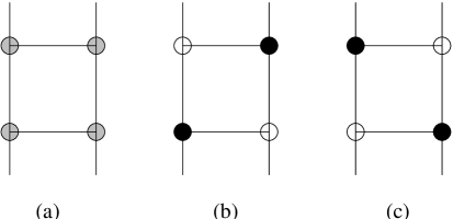
FIG. 2.: Possible (a) disordered and (b), (c) completely charge ordered (zig-zag) configurations in a single ladder. The filled, shaded and open circles denote $V^{+4}$, $V^{+4.5}$ and $V^{+5}$ sites respectively.

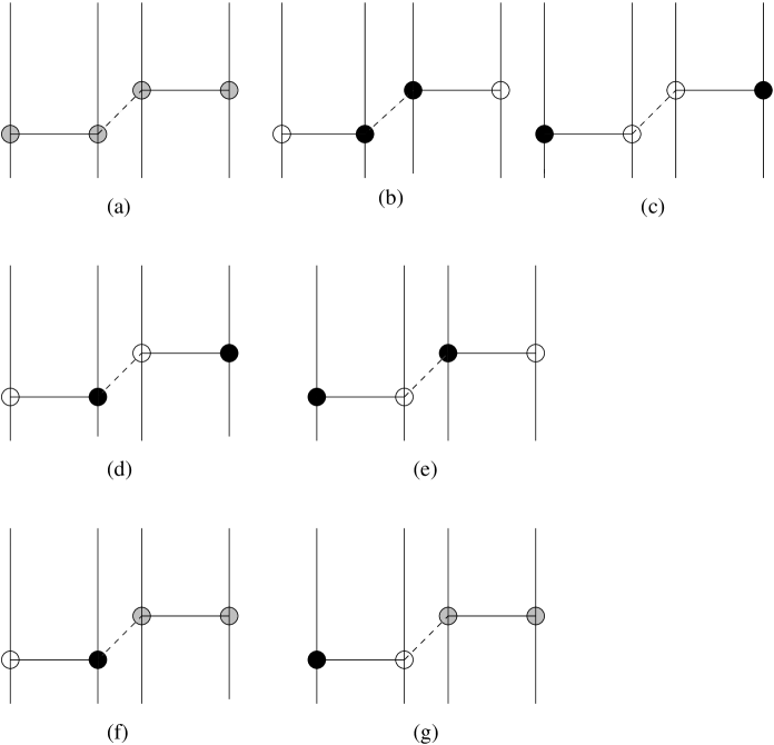
FIG. 3.: Possible (a) disordered; (b), (c), (d), (e) completely charge ordered (zig-zag) and (f), (g) ordered-disordered configurations in between two adjacent ladders.

FIG. 4.: Variations of the effective intra-ladder exchange coupling $J_{eff}^{exch}$ in units of $(t_{b}^{2}/t_{a})$ with respect to the parameter $(V_{a}/2t_{a})$ (for $U=\infty$). Note that the perturbation expansion breaks down at $V_{a}=2t_{a}$.

REFERENCES

• [1] E-mail: debanand@lusi.uni-sb.de
• [2] M. Isobe and Y. Ueda, J. Phys. Soc. Jpn. 65, 1178 (1996).
• [3] M. Weiden, R. Hauptmann, C. Geibel, F. Steglich, M . Fischer, P. Lemmens and G. GΓΌntherodt, Z. Phys. B 103, 1 (1997).
• [4] H. G. von Schnering, Y. Grin, M. Kaupp, M. Sommer R. K. Kremer, O. Jepsen, T. Chatterji and M. Weiden, Z. Kristal. 213, 246 (1998).
• [5] H. Smolinski, C. Gros, W. Weber, U. Peuchert, G. Roth, M. Weiden and C. Geibel, Phys. Rev. Lett. 80, 5164 (1998).
• [6] J. Galy, A. Casalot, M. Pouchard and P. Hagenmuller, C. R. Acad. Sc. Paris. C 262, 1055 (1966).
• [7] T. Ohama, H. Yasuoka, M. Isobe and Y. Ueda, Phys. Rev. B 59, 3299 (1999).
• [8] M. N. Popova, A. B. Sushkov, S. A. Golubchik, B. N. Mavrin, V. N. Denisov, B. Z. Malkin, A. I. Iskhakova, M. Isobe and Y. Ueda, Sissa-cond-mat/9807369.
• [9] P. Thalmeier and P. Fulde, Europhys. Lett. 44, 242 (1998).
• [10] H. Seo and H. Fukuyama, J. Phys. Soc. Jpn. 66, 1249 (1997).
• [11] M. V. Mostovoy and D. I. Khomskii, Sol. St. Comm. 113, 159 (1999).
• [12] C. Gros and R. ValentΓ­, Phys. Rev. Lett. 82, 976 (1999).
• [13] T. Yosihama, M. Nishi, K. Nakajima, K. Kakurai, Y. Fujii, M. Isobe, C. Kagami and Y. Ueda, J. Phys. Soc. Jap. 67, 744 (1998).
• [14] H. Nakao, K. Ohwada, N. Takesue, Y. Fujii, M. Isobe, Y. Ueda, M. v. Zimmermann, J. P. Hill, D. Gibbs, J. C. Woicik, I. Koyama, Y. Murakami, Sissa-cond-mat/0003129.
• [15] J. LΓΌdecke, A. Jobst, S. van Smaalen, E. Morre, C. Geibel and H. -G. Krane, Phys. Rev. Lett. 82, 3633 (1999).
• [16] J. L. de Boer, A. M. Meetsma, J. Baas and T. T. M. Palstra, Preprint, (1999).
• [17] S. van Smaalen and J. LΓΌdecke, Europhys. Lett. 49, 250 (1999).
• [18] C. Gros, R. ValentΓ­, J. V. Alvarez, K. Hamacher and W. Wenzel, preprint (2000).
• [19] T. Ohama, A. Goto, T. Shimizu, E. Ninomiya, H. Sawa, M. Isobe, Y. Ueda, Sissa-cond-mat/0003141.
• [20] K. I. Kugel and D. I. Khomskii, Sov. Phys. JETP. 37, 725 (1973).
• [21] J. R. Schrieffer and P. A. Wolff, Phys. Rev. 149, 491 (1966).
• [22] A. I. Smirnov, M. N. Popova, A. B. Sushkov, S. A. Golubchik, D. I. Khomskii, M. V. Mostovoy, A. N. Vasil’ev, M. Isobe and Y. Ueda, Sissa-cond-mat/9808165.
• [23] P. Horsch and F. Mack, Eur. Phys. J. B 5, 367 (1998).
Refer to caption