The Density Matrix Renormalization Group technique with periodic boundary conditions

Abstract

The Density Matrix Renormalization Group (DMRG) method with periodic boundary conditions is introduced for two dimensional classical spin models. It is shown that this method is more suitable for derivation of the properties of infinite 2D systems than the DMRG with open boundary conditions despite the latter describes much better strips of finite width. For calculation at criticality, phenomenological renormalization at finite strips is used together with a criterion for optimum strip width for a given order of approximation. For this width the critical temperature of 2D Ising model is estimated with seven-digit accuracy for not too large order of approximation. Similar precision is reached for critical indices. These results exceed the accuracy of similar calculations for DMRG with open boundary conditions by several orders of magnitude.

05.70.Fh, 64.70.Rh, 02.60.Dc, 02.70.-c

I Introduction

In 1992 the density matrix renormalization group (DMRG) technique in real space was invented by S. R. White [1] and has been mostly applied to the diagonalization of one-dimensional (1D) quantum chain spin Hamiltonians. Three years later the DMRG method was redesigned by T. Nishino [2] and applied to classical spin 2D models. The DMRG method for the classical models is based on renormalization of the transfer matrix. It is a variational method maximizing the partition function using a limited number of degrees of freedom and its variational state is written as a product of local matrices [3, 4].

DMRG has been used for many various quantum models. It provides results with remarkable accuracy for larger systems than it is possible to study using standard diagonalization methods. The 2D classical systems treated by the DMRG method exceeds the classical Monte Carlo approach in accuracy, speed, and size of the systems [5]. A further DMRG improvement of the classical systems is based on Baxter’s corner transfer matrix [6], the CTMRG [7], and its generalization to any dimension [8].

Applications of the DMRG technique for calculation of the thermodynamic properties in the 2D classical systems has been done by [2, 9, 10, 11]. Treating of non-symmetric transfer matrices or non-hermitian quantum Hamiltonians has also been studied by the DMRG technique [12, 13, 14, 15].

It was shown that DRMG method yields very accurate estimations of ground state energy of finite quantum chains and free energy of classical strips of finite width with open boundary conditions. We have developed the DMRG method with periodic boundary conditions for strips of classical spins and shown that, similarly as for quantum chains, it gives these quantities with much less degree of accuracy. Nevertheless, the DMRG method is mostly used for prediction of physical quantities and critical properties of infinite systems in connection with finite size scaling or extrapolation of the results from finite-size systems to infinite ones. The objective of this paper is to study the DMRG and exact methods with two different boundary conditions for finite strips of various widths and compare their results with known exact results for infinite 2D system. It is shown that while for the exact diagonalization of finite-strip transfer matrices scaling properties of the system improve, for DMRG approach there exists an optimum width for each degree of approximation. The developed approach is tested on 2D Ising model.

Paper is organized as follows: in Sec. II we mention briefly the DMRG for the open boundary conditions; Sec. III contains the modification of the DMRG method for the periodic boundary conditions; in Sec. IV we present the results obtained by the DMRG method with periodic and open boundary conditions, the exact diagonalization method and show how to determine the optimum strip width for finite-size scaling, and in Sec. V the results will be summarized.

II DMRG with open boundary conditions

The transfer matrix approach is a powerful method for exact numerical calculation of thermodynamical properties of lattice spin models defined on finite-width strips. If the width of the strip is too large and the capacity of the computer is exceeded, the DMRG method is found to be useful for an effective reduction of the transfer matrix size. It can be used for calculation of global quantities such as free energy as well as of a spatial dependence across the strip of local quantities, e.g. spin correlation functions.

The properties of an infinite strip of finite width $L$ are given by the solution of ‘left’ eigenvectors and corresponding eigenvalues of the transfer matrix equation

$$\sum\limits_{\{\sigma\}}\Psi_{l}\left(\{\sigma\}\right)T\left(\{\sigma\}|\{\sigma^{\prime}\}\right)=\lambda\Psi_{l}\left(\{\sigma^{\prime}\}\right),$$ (1)

where $\{\sigma\}$ is a set of $L$ spins $\{\sigma_{1},\sigma_{2},\dots,\sigma_{L}\}$ defined on a row and $\{\sigma^{\prime}\}$ is a set of $L$ spins on the adjacent row. The transfer matrix is a product of Boltzmann weights given by the lattice Hamiltonian. For non-symmetric transfer matrices besides the left eigenvectors $\Psi^{i}_{l}$, the right eigenvectors $\Psi^{i}_{r}$ should be calculated, as well.

Reducing the size of the transfer matrix the standard DMRG technique proceeds in two regimes:
(1) In the process of iterations, the infinite system method (ISM) pushes both ends of the transfer matrix further so that each step of the ISM enlarges the lattice size by two sites. The transfer matrix (superblock) is constructed from three blocks: left $T_{l}$ and right $T_{r}$ transfer matrices (blocks) and a Boltzmann weight $W_{B}$, in particular

$$T_{[2j+2]}=T^{(j)}_{l}W_{B}T^{(j)}_{r},$$ (2)

where the index on the left hand side denotes the number of sites in one row of the whole superblock $T$ at the $j$th step of iteration. The Boltzmann weight usually is a function of several spins interacting among each other, e.g. for the Ising model with nearest-neighbor interactions the Boltzmann weight has the form

$$W_{B}(\sigma_{1}\sigma_{2}|\sigma_{1}^{\prime}\sigma_{2}^{\prime})=\exp\left\{-\frac{J}{k_{B}T}(\sigma_{1}\sigma_{2}+\sigma_{1}^{\prime}\sigma_{2}^{\prime}+\sigma_{1}\sigma_{1}^{\prime}+\sigma_{2}\sigma_{2}^{\prime})\right\}.$$ (3)

In the first step of the ISM (for details, see [1, 2]) $T_{l}^{(1)}=T_{r}^{(1)}=W_{B}$ is put. The whole procedure has $L/2-1$ steps

$$T_{l}^{(1)}W_{B}T_{r}^{(1)}\rightarrow T_{l}^{(2)}W_{B}T_{r}^{(2)}\rightarrow\cdots\rightarrow T_{l}^{(L/2-1)}W_{B}T_{r}^{(L/2-1)}.$$ (4)

and stops when the desired strip width of $L$ sites is reached.

The first steps of the iteration scheme (4) are exact but if the superblock matrix $T$ becomes too large, a reduction procedure, to keep the size of superblock constant, should be introduced.

The first step of (4) introduces open conditions at the strip boundaries. If the temperature of the system is lower than the critical one and the strip width is wide enough, the symmetry of the system is spontaneously broken (order parameter becomes non-zero), and after reaching the fixed point of the iteration procedure, the system does not depend on the boundary conditions any more. The calculations with periodic boundary conditions described in the next Section give in this regime the same result as with the free ones.
(2) the finite system method (FSM) improves numerical accuracy of ISM result by left and right moves (sweeps) according to the following prescription:

$$T_{l}^{(L/2-1)}W_{B}T_{r}^{(L/2-1)}\rightarrow T_{l}^{(L/2)}W_{B}T_{r}^{(L/2-2)}\rightarrow\cdots\rightarrow T_{l}^{(L-3)}W_{B}T_{r}^{(1)},$$ (5)

$$T_{l}^{(L-3)}W_{B}T_{r}^{(1)}\rightarrow T_{l}^{(L-2)}W_{B}T_{r}^{(2)}\rightarrow\cdots\rightarrow T_{l}^{(L/2-1)}W_{B}T_{r}^{(L/2-1)}.$$ (6)

In the right sweep (5) the left blocks $T_{l}$ are calculated in the previous step of the sweep and the right blocks $T_{r}$ are taken from the previous left sweep (in the first right sweep from ISM); similarly for the left sweep.

The values of local thermodynamical quantities given by particular superblocks in the final sweep (after the steady state is reached) are spatially dependent. The values given by the superblock in the middle of the strip $T_{l}^{(L/2-1)}W_{B}T_{r}^{(L/2-1)}$ are the closest to the bulk ones. In this sense, the best transfer matrix eigenvalues as well as eigenvectors are those of the above-mentioned central superblock. The two largest eigenvalues are used for further finite-size scaling or extrapolation treatment.

III DMRG with periodic boundary conditions

The translational invariance of the infinite lattice is preserved in finite strips with periodic boundary conditions when strip boundaries are connected with bulk intersite interactions. In this case the strip forms an infinitely long cylinder. If the radius of the cylinder is small enough, the model can be easily solved by exact numerical diagonalization methods.

In DMRG language, imposing periodic boundary conditions means that we have to introduce properly the connection of both ends of the superblock transfer matrix $T$. Thus, in distinction to open-boundary case the superblock is constructed from two Boltzmann weights connecting two blocks at both ends (see Fig. 1, the rightmost diagram).

$$T_{[2j+4]}(\sigma_{1}\xi_{l}\sigma_{j+4}\sigma_{j+3}\xi_{r}\sigma_{2}|\sigma_{1}^{\prime}\xi_{l}^{\prime}\sigma_{j+4}^{\prime}\sigma_{j+3}^{\prime}\xi_{r}^{\prime}\sigma_{2}^{\prime})=T_{l}^{(j)}(\sigma_{1}\xi_{l}\sigma_{j+4}|\sigma_{1}^{\prime}\xi_{l}^{\prime}\sigma_{j+4}^{\prime})$$ (7)

$$\times W_{B}(\sigma_{j+4}\sigma_{j+3}|\sigma_{j+4}^{\prime}\sigma_{j+3}^{\prime})T_{r}^{(j)}(\sigma_{j+3}\xi_{r}\sigma_{2}|\sigma_{j+3}^{\prime}\xi_{r}^{\prime}\sigma_{2}^{\prime})W_{B}(\sigma_{2}\sigma_{1}|\sigma_{2}^{\prime}\sigma_{1}^{\prime}),$$ (8)

where the block spin variable $\xi=\{1,2,\dots,m\}$, and the primed variables are denoted by filled circles and ovals in Fig. 1.

In the first few steps the lattice is enlarged to the desired size; no degrees-of-freedom reduction is performed and the superblock transfer matrix remains equivalent to the exact one. As depicted in Fig. 1, the ISM starts with $T^{(6)}=T_{l}^{(1)}W_{B}T_{r}^{(1)}W_{B}$ defined on twelve sites where $T_{l}^{(1)}=T_{r}^{(1)}=W_{B}W_{B}$, and one Boltzmann weight, i.e. four new sites are added in each of further steps.

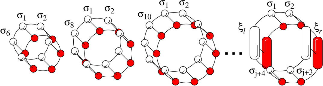
FIG. 1.: The first $j$ steps of the ISM for the strip with the periodic boundary conditions.

If $2^{j}>m$, the number of degrees of freedom should be reduced at each $j$th step to keep the order of the superblock matrix constant and equal to $2^{4}\cdot m^{2}$.

Summation in the equation for eigenvectors (1) of the transfer matrix (8) can be performed in two steps

$$\Phi(\sigma_{1}\xi_{l}\sigma_{j+4}\sigma_{j+3}\sigma_{j+3}^{\prime}\xi_{r}^{\prime}\sigma_{2}^{\prime}\sigma_{1}^{\prime}) = \sum\limits_{\xi_{r}\sigma_{2}}T_{r}(\sigma_{j+3}\xi_{r}\sigma_{2}|\sigma_{j+3}^{\prime}\xi_{r}^{\prime}\sigma_{2}^{\prime})W_{B}(\sigma_{2}\sigma_{1}|\sigma_{2}^{\prime}\sigma_{1}^{\prime})$$ (10)

$$\times\Psi(\sigma_{1}\xi_{l}\sigma_{j+4}\sigma_{j+3}\xi_{r}\sigma_{2})$$

$$\Psi(\sigma_{1}^{\prime}\xi_{l}^{\prime}\sigma_{j+4}^{\prime}\sigma_{j+3}^{\prime}\xi_{r}^{\prime}\sigma_{2}^{\prime}) = \sum\limits_{{\sigma_{1}\xi_{l}}\atop{\sigma_{j+4}\sigma_{j+3}}}T_{l}(\sigma_{1}\xi_{l}\sigma_{j+4}|\sigma_{1}^{\prime}\xi_{l}^{\prime}\sigma_{j+4}^{\prime})W_{B}(\sigma_{j+4}\sigma_{j+3}|\sigma_{j+4}^{\prime}\sigma_{j+3}^{\prime})$$ (12)

$$\times\Phi(\sigma_{1}\xi_{l}\sigma_{j+4}\sigma_{j+3}\sigma_{j+3}^{\prime}\xi_{r}^{\prime}\sigma_{2}^{\prime}\sigma_{1}^{\prime})$$

which is depicted graphically in Fig. 2.

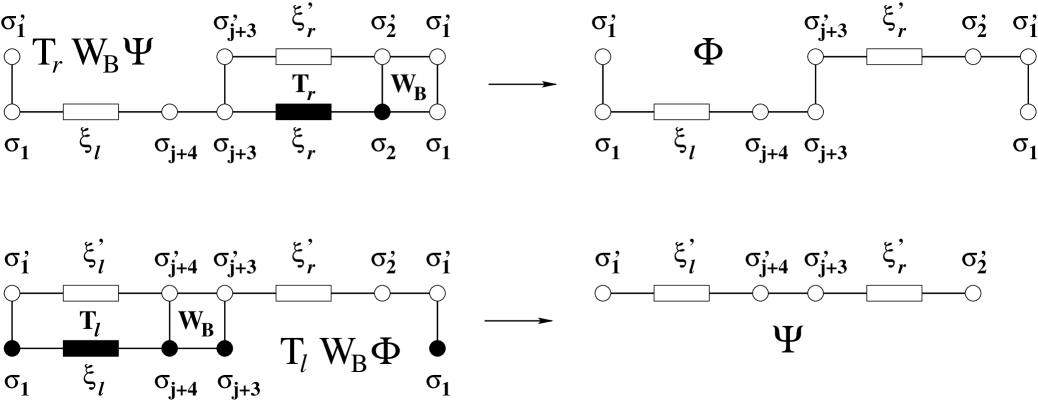
FIG. 2.: Graphical representation of Eq. (12). The variables represented by filled circles and rectangles are summed over. The spins $\sigma_{1}$ and $\sigma_{1}^{\prime}$ at both ends of the superblock must be identified due to the periodic boundary conditions.

This procedure uses the left and right transfer matrix blocks to calculate properly the left and right eigenvectors $\Psi_{l}$ and $\Psi_{r}$, respectively, of the whole superblock for the periodic boundary conditions. Once we have the $\Psi_{l}$ and $\Psi_{r}$, the left and right density matrices can be constructed.

$$\rho_{l}(\xi_{l}\sigma_{j+4}|\xi_{l}^{\prime}\sigma_{j+4}^{\prime})=\sum\limits_{\sigma_{1}\sigma_{j+3}\xi_{r}\sigma_{2}}\Psi_{l}(\sigma_{1}\xi_{l}\sigma_{j+4}\sigma_{j+3}\xi_{r}\sigma_{2})\Psi_{r}(\sigma_{1}\xi_{l}^{\prime}\sigma_{j+4}^{\prime}\sigma_{j+3}\xi_{r}\sigma_{2})$$ (13)

$$\rho_{r}(\sigma_{j+3}\xi_{r}|\sigma_{j+3}^{\prime}\xi_{r}^{\prime})=\sum\limits_{\sigma_{1}\xi_{l}\sigma_{j+4}\sigma_{2}}\Psi_{l}(\sigma_{1}\xi_{l}\sigma_{j+4}\sigma_{j+3}\xi_{r}\sigma_{2})\Psi_{r}(\sigma_{1}\xi_{l}\sigma_{j+4}\sigma_{j+3}^{\prime}\xi_{r}^{\prime}\sigma_{2}),$$ (14)

and by its complete diagonalization

$$O_{l}(\xi_{l}^{new}|\xi_{l}\sigma_{j+4})\rho_{l}(\xi_{l}\sigma_{j+4}|\xi_{l}^{\prime}\sigma_{j+4}^{\prime})Q_{l}(\xi_{l}^{\prime}\sigma_{j+4}^{\prime}|\xi_{l}^{\prime\ new})=\omega_{i}\delta_{ij}$$ (15)

sets of left and right eigenvectors stored in $O_{l}$ and $Q_{l}$ matrices, respectively, is obtained (analogously, for $O_{r}$ and $Q_{r}$). The indices $i,j$ ($i,j\!=\!1,2,\dots,2m$) run over all states of $m$-state multi-spin variable $\xi$ and two-state variable $\sigma$. For the last steps of ISM and all FSM steps half of the eigenvectors (corresponding to their lowest eigenvalues) is discarded from the matrices $O$ and $Q$, and the information of the system carried by the density matrix is reduced. However, remaining eigenvectors (if $m$ is large enough) usually describe the system accurately because the truncation error $\varepsilon$ defined as

$$\varepsilon=\sum\limits_{\{{\rm discarded}\}}\omega$$ (16)

is very small ($0\leq\varepsilon\ll 1$). $\sum_{\{all\}}\omega\!=\!1$, as the eigenvectors are assumed to be normalized. The matrices $O$ and $Q$ enter the linear transformation as projectors mapping two blocks $T_{l}W_{B}$ onto one block $T_{l}$ through the following procedure

$$T_{l}^{(j+1)}(\sigma_{1}\xi_{l}^{new}\sigma_{j+5}|\sigma_{1}^{\prime}\xi_{l}^{\prime\ new}\sigma_{j+5}^{\prime})=\sum\limits_{{\xi_{l}^{\prime}\sigma_{j+4}^{\prime}}\atop{\xi_{l}\sigma_{j+4}}} O_{l}(\xi_{l}^{new}|\xi_{l}\sigma_{j+4})T_{l}^{(j)}(\sigma_{1}\xi_{l}\sigma_{j+4}|\sigma_{1}^{\prime}\xi_{l}^{\prime}\sigma_{j+4}^{\prime})$$ (17)

$$\times W_{B}(\sigma_{j+4}\sigma_{j+5}|\sigma_{j+4}^{\prime}\sigma_{j+5}^{\prime})Q_{l}(\xi_{l}^{\prime}\sigma_{j+4}^{\prime}|\xi_{l}^{\prime\ new}).$$ (18)

Application to the right block $T_{r}$ is straightforward. As it is seen, we calculate the blocks $T_{l}$ and $T_{r}$ separately not using the standard mirror-reflection of $T_{l}$ to $T_{r}$. This procedure is necessary when dealing with anisotropic and/or inhomogeneous systems.

The calculated new blocks $T_{l}^{(j+1)}$ and $T_{r}^{(j+1)}$ are used in the next step of the ISM for construction of the new superblock

$$T_{[2j+6]}=T_{l}^{(j+1)}W_{B}T_{r}^{(j+1)}W_{B}.$$ (19)

Within the FSM, e.g., for a sweep to the right only the left blocks are calculated and $T_{r}^{(L/2-k)}$ is taken from the previous left sweep

$$T_{[L]}=T_{l}^{(L/2-3+k)}W_{B}T_{r}^{(L/2-1-k)}W_{B}.$$ (20)

The variable $k$ (indexing the steps within a sweep) runs over the values $(-k_{0},-k_{0}+1,\dots,k_{0}-1,k_{0})$, where $2^{k_{0}}\leq 2^{L/2-2}-m$. In the process of sweeping one of the Boltzmann weight is fixed (the upper one in Fig. 1) and the second one changes its position within the interval of $2k_{0}$ lattice sites. The local physical quantities are calculated at the lattice sites of the fixed Boltzmann weight and due to the rotational invariance of the problem are valid for all the rows of the periodic lattice.

IV Results

It is well known that the DMRG describes better a strip with open boundary conditions than that with the periodic boundary conditions [1] because the precision of the largest eigenvalue of the superblock matrix is increasing proportionally to $m$ for open boundary conditions while for periodic boundary conditions only as $\sqrt{m}$.

However, if we are not interested in the largest eigenvalue of a finite-strip transfer matrix but in the estimation of the free energy of the whole 2D lattice (per spin), it is more effective to use a strip with periodic boundary conditions than that with open boundaries, as demonstrated in Table 3. The results with $m=25$ practically exactly reproduce the exact values for $L=16$. The estimation of the free energy for 2D models performed by DMRG can be improved by increasing the width of the strip. For a given $m$ the best results are obtained for $L\rightarrow\infty$, but in this case, for $T=2.1$ (i.e. below the critical temperature), the symmetry of the system is spontaneously broken. Exact free energy per site $f^{\rm(exact)}_{\rm Onsager}$ was taken from [16].

FIG. 3.: Free energy per site $f_{\rm ISM}$ for the Ising model calculated with the standard DMRG method only with the ISM is compared with the free energy per site calculated by the modified DMRG algorithm as well as by the exact diagonalization method (EDM). $N$ is the order of either the superblock of DMRG or the exact transfer matrix in EDM.

The critical temperature and the properties of the infinite 2D system near the critical temperature should be derived from finite-size scaling ideas (as the finite-width strip is at criticality for $T=0$ only).

For calculation of the critical temperature, the phenomenological renormalization approach of Nightingale [17] have been used. Here, the scaling properties of the correlation length, found as logarithm of the ratio of two largest eigenvalues of the exact or superblock matrix, are exploited. The product of the inverse correlation length $K_{N}$ and the strip width $L$ should not depend on the $L$ at critical temperature $T_{\rm C}^{*}(L)$

$$\frac{LK_{L}}{(L+2)K_{L+2}}=1.$$ (21)

The accuracy of the approximate critical temperature improves with size of the strip in the case of exact diagonalization. For DMRG calculations this statement is no longer valid, as for very large $L$ the symmetry of the system spontaneously breaks, and the phenomenological renormalization is not applicable any more. Thus, for given order of approximation $m$, there exists an optimum value of the strip width $L^{\rm opt}$. This can be estimated from the following considerations: For exact diagonalization or DMRG calculations with $m$ close to $2^{L/2-2}$, the difference of the approximate critical temperature from the exact critical temperature $T_{\rm C}^{\rm(exact)}=2\ln^{-1}(1+\sqrt{2})$ [19] scales with the width of the strip as follows [18]:

$$\frac{T_{\rm C}^{*}(L)-T_{\rm C}^{(\rm exact)}}{T_{\rm C}^{(\rm exact)}}\sim L^{-1/\nu},$$ (22)

i.e. the ratio

$$R\equiv\frac{\frac{{\rm d}}{{\rm d}L}T_{\rm C}^{*}(L)}{\frac{{\rm d}^{2}}{{\rm d}L^{2}}T_{\rm C}^{*}(L)}=\frac{\nu}{\nu+1}L\sim L.$$ (23)

The optimum width $L^{\rm opt}$ should be less than $L_{\rm C}$ for which the ratio of the derivatives $R(L_{\rm C})$ (23) is substantially deviated from the originally linear behavior. In our calculations we have considered the DMRG results to be incorrect for $R=0$ or $\infty$. In the case of $R=0$, the precise value of $L^{\rm opt}$ is not too important as the first derivative or change of $T_{\rm C}^{*}(L)$ is very small. Near $R=\infty$, a sharp drop of the second derivative of $T_{\rm C}^{*}(L)$ to zero is required; indeed, the change of the distance from the line ${\nu\over\nu+1}L$ by more than one order of magnitude takes place within one step of strip-width enlargement.

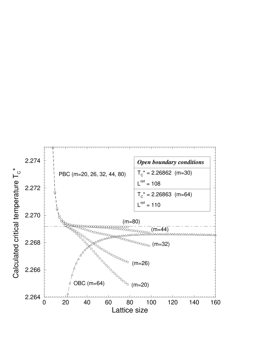
FIG. 4.: Critical temperatures $T_{\rm C}^{*}$ for Ising model as functions of lattice size $L$ for various sizes of multi-spin variables $m$ from DMRG and finite-size scaling. The results for open boundary conditions (OBC) are plotted as triangles while the results for the periodic boundary conditions (PBC) are plotted as circles. The exact critical temperature is at the dot-dashed line. The OBC plot for $m=30$ is indistinguishable from the curve for $m=64$ in this figure.

In Fig. 4 plots of strip-width-dependent critical temperatures $T_{\rm C}^{*}(L)$ for two different boundary conditions and various block sizes $m$ are given. The estimations of the exact critical temperature for periodic and open boundary conditions were found as the values of $T_{\rm C}^{*}(L-2)$ if the first or second derivative of $T_{\rm C}^{*}(L)$ changed their signs with respect to the value in the previous step. The curves for PBC cross the exact value of $T_{\rm C}^{\rm(exact)}$. The curve maxima for OBC are quite far from it, and by increasing $L$, $T_{\rm C}^{*}$ approaches the exact value very slowly.

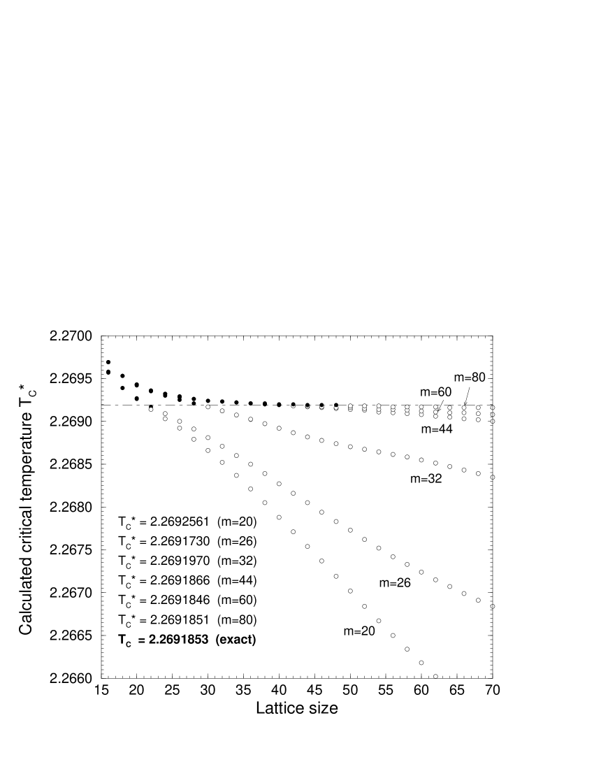
FIG. 5.: Critical temperatures $T_{\rm C}^{*}$ in Ising model vs. lattice size $L$ and $m$ for the periodic boundary conditions (PBC) only. Filled circles represents data which are accepted whereas the open circles are taken as incorrect due to violation of the condition (23). Zoomed Fig. 4. The critical temperature estimations in the inset are given by the rightmost filled circles for respective $m$.

The accuracy of the results for periodic boundary conditions (Fig. 5) is very high already at small values of $m$ and exceeds by an order the critical temperature estimation for maximum computer-accessible $m$ when using open boundary conditions. The critical temperature for not extremely large $m=80$ is given to seven digits. As the width of the strip can be increased only in discrete steps and the criterion of the optimum strip-width is somewhat vague, the accuracy of the critical temperature determination should be taken as large as a single step change of $T_{\rm C}^{*}(L)$. These accuracy estimations together with deviations of our results from the exact critical temperature are given in Table 6. It should be noted that only ISM was performed in calculations of $T_{\rm C}^{*}(L)$ in Figs. 4 and 5. The calculations with the FSM has been also done near the $L^{\rm opt}$ but only slight improvements of critical temperature were obtained. In calculation of the thermal critical exponent [17] a similar accuracy was reached; e.g., for $m=44$ within FSM the critical exponent $\nu=1.0000016$ is very close to the exact value $\nu=1$ [19].

FIG. 6.: Changes of $T_{\rm C}^{*}(L)$ per one step of strip-width enlargement as well as the deviations of our results from the exact critical temperature $T_{\rm C}^{\rm(exact)}$ for increasing parameter $m$.

V Conclusion

The DMRG method for classical spin lattice strips with periodic boundaries was developed and applied to 2D Ising model. It was shown that this approach lead to more accurate results for 2D infinite lattice than DMRG with open boundary conditions. It was demonstrated that applying finite size scaling to strips treated by DMRG, an optimal width of the strip depending on the order of approximation existed, and a prescription how to find $T_{\rm C}^{*}(L^{\rm opt})$ was given. For the Ising model it was shown by computations that for these $L^{\rm opt}(m)$ the value of the critical temperature, was for a given $m$ closest to the exact one. As our approach does not involve any information about the exact critical temperature $T_{\rm C}^{\rm(exact)}$ or the universality class of the model, we believe that it is applicable to many different classes of spin lattice models. This belief is supported by analogous calculation for anisotropic triangular nearest-neighbor Ising model (ATNNI) with two different antiferromagnetic interactions $J_{1}$ and $J_{2}$ (model discussed in [15]). For this model the transfer matrix is non-symmetric and the phase diagram is quite different from that of the standard Ising model. For the periodic boundary conditions, the plot of critical temperatures is not monotonously decreasing as in the case of the Ising model (Fig. 5) but for large $L$ it turns up. Nevertheless, the accuracy of the critical temperature for the exactly solvable case (for external magnetic field $H=0$) is similar to the presented ones in this paper.

REFERENCES

- [1] S. R. White, Phys. Rev. Lett. 69, 2863 (1992); Phys. Rev. B 48 10345 (1993).
- [2] T. Nishino, J. Phys. Soc. Jpn. 64, 3598 (1995).
- [3] S. Östlund and S. Rommer, Phys. Rev. Lett. 75, 3537 (1995); Phys. Rev. B 55, 2164 (1997); K. Okunishi, Y. Hieida and Y. Akutsu, cond–mat/9810239.
- [4] A. Šurda, Acta Phys. Slov. 49, 325 (1999).
- [5] K. Hallberg, cond–mat/9910082.
- [6] R. Baxter, J. Math. Phys. 9, 650 (1968); J. Stat. Phys. 19, 461 (1978).
- [7] T. Nishino and K. Okunishi, J. Phys. Soc. Jpn. 65 891 (1996); Phys. Soc. Jpn. 66 3040 (1997); T. Nishino, K. Okunishi and M. Kikuchi, Phys. Lett. A 213, 69 (1996).
- [8] T. Nishino and K. Okunishi, J. Phys. Soc. Jpn. 67, 3066 (1998).
- [9] E. Carlon and A. Drzewiǹski, Phys. Rev. Lett. 79, 1591 (1997).
- [10] T. Nishino and K. Okunishi, J. Phys. Soc. Jpn. 64 4084 (1995).
- [11] Y. Honda and T. Horiguchi, Phys. Rev. E 56, 3920 (1997).
- [12] Y. Hieida, J. Phys. Soc. Jpn. 67, 369 (1998), Y. Hieida, K. Okunishi and Y.Akutsu, New J. Phys. 1 7.1 (1999).
- [13] T. Nishino and N. Shibata, J. Phys. Soc. Jpn. 68, 3501 (1999); N. Shibata, J. Phys. Soc. Jpn. 66, 2221 (1997); X. Wang and T. Xiang, Phys. Rev. B 56, 5061 (1997); R. J. Burssil, T. Xiang and G. A. Gehring, J. Phys. Cond. Mat. 8, L583 (1996); K. Maisinger and U. Schollwöck, Phys. Rev. Lett. 81, 445 (1998).
- [14] E. Carlon, M. Henkel, and U. Schollwöck, Eur. Phys. J. B12, 99 (1999).
- [15] A. Gendiar, A. Šurda, to appear in Phys. Rev. B.
- [16] L. D. Landau and E. M. Lifshitz, Statistical physics, Vol. 5, Nauka, Moscow (1964).
- [17] P. Nightingale, J. Appl. Phys. 53, 7927 (1982).
- [18] M. N. Barber, in Phase Transitions and Critical Phenomena, edited by C. Domb and J. L. Lebowitz, (Academic Press, London, 1983), Vol 8, pp. 146-266.
- [19] R. J. Baxter, Exactly Solved Models in Statistical Physics, Academic Press, London (1982).