Effect of incoherent scattering on shot noise correlations in the quantum Hall regime

Abstract

We investigate the effect of incoherent scattering in a Hanbury Brown and Twiss situation with electrons in edge states of a three-terminal conductor submitted to a strong perpendicular magnetic field. The modelization of incoherent scattering is performed by introducing an additional voltage probe through which the current is kept equal to zero which causes voltage fluctuations at this probe. It is shown that inelastic scattering can lead in this framework to positive correlations, whereas correlations remain always negative for quasi-elastic scattering.

]

I Introduction

The effect of incoherent scattering on transport and noise in mesoscopic structures has been of interest in a number of previous works (for review see [1, 2]). In this paper we are interested in the effect of inelastic and quasi-elastic scattering on the correlations of the current in a structure submitted to a strong magnetic field so that the current is carried by edge states propagating along the boundary of the sample (see figure 1).

To demonstrate the reality of edge states [3] (despite their small contribution to the overall density of states) the possibility of creating a non-equilibrium population [4] has been crucial. Several experiments have investigated the equilibration of edge states selectively populated with the help of various contacts by transport measurements [5, 6, 7, 8]. A natural problem is to investigate the effect of inter-edge state scattering on the noise on such structures.

Recently, Hanbury Brown and Twiss (HBT) experiments studying current correlations using partially degenerate stream of fermions were performed [9, 10], starting from the idea [11] of using the edge states in a conductor submitted to a strong magnetic field. A Y-structure is discussed in Ref. [12] and a HBT experiment without a magnetic field has also been realized [13]. Here we are interested in the experimental arrangement of Oberholzer et al. [10] which is depicted in figure 1, with the only difference that the magnetic field, in this experiment, was adjusted in such a way that only one spin-degenerate edge state (filling factor $\nu=2$) carries the current, and not two, as it is represented on the figure. Contact 1, which is at a potential $eV$ above the potentials of the two other contacts, acts as a carrier source and contacts 2 and 3 as detectors for the beams of electrons. The incident beam is splitted at two quantum point contacts (QPC) which can be tuned by applied voltages. In the following we will denote by $T_{1}$ and $R_{1}=1-T_{1}$ the transmission and reflection coefficients at QPC at contact 1, and introduce $T_{3}$ and $R_{3}$ for QPC at contact 3. The quantity of interest in this experiment, revealing statistical properties of the carriers, is the correlation $S_{23}=\left\langle\Delta I_{2}\Delta I_{3}\right\rangle$ between the current at the two contacts. Compared to the initial experiment by Henny et al. [9] the experiment by Oberholzer et al. [10] introduces fluctuations in the incident beam and thus the current correlations are not determined already from current conservation alone. In the following we will be interested in the case where the distance between the QPC’s is long so that incoherent processes may occur along this edge. If only one edge state is populated, phase breaking processes are of little interest since $S_{23}$ measures quantum-statistical properties of the carriers revealed by the separation of the beam at QPC 3, and what happens before this separation is of little importance. We can indeed check that the introduction of incoherent processes within the framework that will be used in the following does not affect the auto-correlations (noise) and the correlations if only one edge state is present.

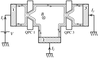
FIG. 1.: Experimental arrangement of [10]. The two edge states are populated at contact 1. One of those channels is perfectly transmitted the other being partially transmitted at QPC 1. The transmission may be tuned by an applied gate voltage. QPC 3 splits the partially degenerate beam and distributes the current to contacts 2 and 3 where it is measured. Without inter-edge state scattering, the perfectly transmitted channel does not manifest itself on the correlations.

In contrast, when several edge states are populated, inter-edge state scattering along one boundary may cause a redistribution of the carriers between the edge states and thus modify the noise properties of each channel. This is the situation that will interest us in this paper. Inter-edge state scattering centers were investigated experimentally very recently [14]. We will not take into account the spin degeneracy which only would multiply the conductances and the noise by a factor 2.

The inelastic [15, 16, 1] and quasi-elastic scattering [1, 17] are modeled by introducing an additional probe at the edge along which incoherent scattering occurs (see figure 2). We have to impose that the current through this probe is zero at any time. This approach, followed in a number of works [1, 15, 17, 18, 19, 20, 21, 22] (see [2] for a review), has the advantage to reduce the problem to the study of coherent scattering in a conductor with one additional contact. The method will be recalled in more detail in the following.

In the first section we are interested in the situation where only coherent scattering is present. In the following section we describe the influence of incoherent scattering along the long edge of the sample.

II Coherent Scattering

We first discuss the situation when only elastic scattering is present in the system. We consider the situation depicted in figure 1 where the magnetic field is chosen so that two edge states are populated. The edge state associated with the lowest Landau level (LL) is perfectly transmitted at the two QPC’s whereas the second edge state associated with the second LL is only partially transmitted at the QPC’s. We are interested in the current correlations between contacts 2 and 3.

The noise spectrum is defined as $S_{\alpha\beta}(\omega)2\pi\delta(\omega+\omega^{\prime})=\langle\Delta\hat{I}_{\alpha}(\omega)\Delta\hat{I}_{\beta}(\omega^{\prime})+\Delta\hat{I}_{\beta}(\omega^{\prime})\Delta\hat{I}_{\alpha}(\omega)\rangle$ with $\Delta\hat{I}_{\alpha}(\omega)=\hat{I}_{\alpha}(\omega)-\langle\hat{I}_{\alpha}(\omega)\rangle$, where $\hat{I}_{\alpha}(\omega)$ is the Fourier transform of the current operator at contact $\alpha$. (For a recent presentation of the formalism and notations, see [2]). The zero frequency limit will be denoted: $S_{\alpha\beta}=S_{\alpha\beta}(\omega=0)$. Following the scattering approach, we construct the scattering matrix for the system to calculate the noise [23, 2]:

$$S_{\alpha\beta}=\frac{2e^{2}}{h}\int{\rm d}E\,\sum_{\gamma,\lambda}\mathop{\mathrm{Tr}}\nolimits\left\{A_{\gamma\lambda}^{\alpha}A_{\lambda\gamma}^{\beta}\right\}f_{\gamma}(1-f_{\lambda})\>,$$ (1)

where the matrices $A$’s are related to the on-shell $S$-matrix: $A_{\gamma\lambda}^{\alpha}=\delta_{\alpha\gamma}\delta_{\alpha\lambda}-s^{\dagger}_{\alpha\gamma}(E)s_{\alpha\lambda}(E)$, $f_{\alpha}$ being the Fermi-Dirac distribution at the contact $\alpha$. We consider the case of zero temperature and will discuss at the end the effect of temperature on some of the results.

Using this expression and the $S$-matrix we can compute the correlations between the currents at contacts $2$ and $3$, which is eventually found to be [10]:

$$S_{23}=-\frac{2e^{2}}{h}|eV|R_{3}T_{3}T_{1}^{2}\>,$$ (2)

where $R_{1}$, $T_{1}$ and $R_{3}$, $T_{3}$ are the reflection and transmission coefficients for the edge state corresponding to the second LL at QPC 1 and 3, respectively. Since the first edge state is totally transmitted through QPC’s, it carries a noiseless current and does not contribute to the noise or to the correlations. The $R_{3}T_{3}$ factor is the usual partition factor due to the separation of the electron beam at QPC 3. The $T_{1}^{2}$ term is due to the fact that the processes leading to correlations between contacts 2 and 3 involve two electrons transmitted through the QPC 1, which happens with probability $T_{1}^{2}$.

Before discussing the effect of inelastic and quasi-elastic scattering, we may consider first the effect of coherent scattering between the two edge states along the upper edge. This question might seem academic but it will be important to have this result in mind, to appreciate the difference in the correlations $S_{23}$ when the two edge states exchange carriers coherently or incoherently. Let us recall that in the presence of coherent scattering, it was proven that correlations between two contacts are always negative as a consequence of the fermionic nature of the carriers [23]. To describe coherent scattering between edge states we introduce the probability $\varepsilon$ that an electron, starting in one of the two channels, is scattered into the other edge state when it travels between the two QPC’s. Here we do not need to enter into more details about the scattering however let us mention that it has been studied within a microscopic approach in [24, 25]. After having constructed the $S$-matrix, formula (1) gives the correlations:

$$S^{\rm coh}_{23}=-\frac{2e^{2}}{h}|eV|R_{3}\Big{[}(1-\varepsilon)^{2}T_{3}T_{1}^{2}+\varepsilon^{2}T_{3}$$ (3)

$$+\varepsilon(1-\varepsilon)(1-2R_{3}T_{1}+T_{1}^{2})\Big{]}\>.$$ (4)

Let us now discuss a few limiting cases. If $\varepsilon=0$ (no inter-edge state elastic scattering) we fall back to the previous situation (2). If $\varepsilon=1$, the two edge states are perfectly exchanged between the QPC’s and the current separated by QPC 3 issues from the first edge state, perfectly transmitted at QPC 1 and we have simply $S^{\rm coh}_{23}=-\frac{2e^{2}}{h}|eV|R_{3}T_{3}$. Note that the outer edge state in contact 3 is not noiseless but these fluctuations are not correlated with fluctuations at contact 2 and then do not contribute to $S_{23}$ since this edge state is not splitted at QPC 3.

If $T_{1}=0$ the correlation is $S^{\rm coh}_{23}=-\frac{2e^{2}}{h}|eV|[R_{3}T_{3}\varepsilon^{2}+\varepsilon(1-\varepsilon)R_{3}]$. The first term is the partition noise for the beam separated at QPC 3; this term is proportional to the probability $\varepsilon^{2}$ that two electrons are transmitted from the first edge state to the second. The second term is the partition noise due to the separation of the beam between QPC’s. In this process, after the separation of the beam, one electron is transmitted with probability $1$ in the first edge state towards contact 3 and the other is reflected with probability $R_{3}$ towards contact 2.

Another interesting case occurs for $T_{3}=0$. Then the two edge states are perfectly separated at QPC 3. The first edge state flows towards contact 3 whereas the second goes to contact 2. This situation is particularly interesting since it allows us to study separately the noise spectrum of each edge state after having travelled along the upper edge of the conductor. In the absence of scattering between edge states, the currents remain uncorrelated, whereas if redistribution of charges occurs between edge states, it may induce correlations. For coherent scattering, we find: $S^{\rm coh}_{23}=-\frac{2e^{2}}{h}|eV|\varepsilon(1-\varepsilon)R_{1}^{2}$. The only separation of the beam that can cause correlations occurs along the edge with usual partition factor $\varepsilon(1-\varepsilon)$; the factor $R_{1}^{2}$ ensures that, if the currents in the two channels are noiseless before exchanging carriers along the upper edge, they remain noiseless and uncorrelated. Let us also give the currents auto-correlations: $S^{\rm coh}_{22}=\frac{2e^{2}}{h}|eV|[R_{1}T_{1}(1-\varepsilon)^{2}+\varepsilon(1-\varepsilon)R_{1}]$ and $S^{\rm coh}_{33}=\frac{2e^{2}}{h}|eV|[R_{1}T_{1}\varepsilon^{2}+\varepsilon(1-\varepsilon)R_{1}]$. The noise spectral densities have contributions from the splitting of the beam at the first QPC and from the redistribution of the charges between the QPC’s. Let us finally mention the value of the noise when $\varepsilon=1/2$, i.e. when the average currents in the two edge states are equally equilibrated due to scattering, then

$$S^{\rm coh}_{23}=-\frac{e^{2}}{h}|eV|\frac{R_{1}^{2}}{2}\hskip 14.22636pt\mbox{ for }T_{3}=0,\ \varepsilon=1/2$$ (5)

and

$$S^{\rm coh}_{22}=S^{\rm coh}_{33}=\frac{e^{2}}{h}|eV|\frac{1+T_{1}}{2}{R_{1}}\>.$$ (6)

Next we proceed to treat incoherent scattering.

III Introduction of incoherent scattering

As we have already evoked, the presence of inelastic or quasi-elastic scattering will be treated by adding a fictitious contact at the edge along which incoherent scattering is expected to occur [15, 1, 2]. Let us remark that the only place where it can have some influence on the correlations is the edge between the two QPC’s where we have introduced it (see figure 2). Since the current is obviously conserved along the edge, we have to impose that the current $I_{4}$ through this contact is zero at any time. The consequence is that the potential $\mu_{4}$ at this probe is fluctuating.

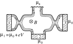
FIG. 2.: Modelization of phase breaking processes along the upper edge.

The average currents are related to the potentials by the conductance: $\left\langle I_{\alpha}\right\rangle=\frac{1}{e}\int{\rm d}E\,\sum_{\beta}G_{\alpha\beta}(E)\bar{f}_{\beta}(E)$, where we recall that $G_{\alpha\beta}=\frac{e^{2}}{h}(N_{\alpha}\delta_{\alpha\beta}-\mathop{\mathrm{Tr}}\nolimits\{s^{\dagger}_{\alpha\beta}s_{\alpha\beta}\})$, $N_{\alpha}$ being the number of open channels at contact $\alpha$. We first discuss the inelastic case [15] for which we require that the current is zero on average $\left\langle I_{4}\right\rangle=0$ and that the average distribution function at the fictitious contact is an equilibrium Fermi distribution. This leads to the following expression for the average chemical potential at contact $4$:

$$\bar{\mu}_{4}=\mu_{0}+\frac{1+T_{1}}{2}eV\>.$$ (7)

The fact that $I_{4}$ is zero on average determines the average distribution function at contact $4$. We have also to ensure that the fluctuating part of $I_{4}$ remains zero. At contact $\alpha$ the current may be written as $I_{\alpha}=\frac{1}{e}\int{\rm d}E\,\sum_{\beta}G_{\alpha\beta}f_{\beta}+\delta I_{\alpha}$, where $\delta I_{\alpha}$ is the intrinsic part of the fluctuations, whose spectrum is given by (1). We now write the currents as $I_{\alpha}=\left\langle I_{\alpha}\right\rangle+\Delta I_{\alpha}$. Imposing that the fluctuating current is zero $\Delta I_{4}=0$ leads to the relation $\delta I_{4}=-\frac{1}{e}G_{44}(\mu_{4}-\bar{\mu}_{4})$ which gives the expression of the fluctuating part of the current:

$$\Delta I_{\alpha}=\delta I_{\alpha}-\frac{G_{\alpha 4}}{G_{44}}\delta I_{4}\>,$$ (8)

the first term corresponds to intrinsic fluctuations of the current and the second term to the fluctuations due to the existence of a fluctuating potential at contact $4$.

In the quasi-elastic case [1] we impose that not only the total current $I_{4}=\int{\rm d}E\,j_{4}(E)$ is zero on average but the contribution to the current of the states of energy $E$ is zero $\left\langle j_{4}(E)\right\rangle=0$, which gives the averaged distribution function at contact $4$:

$$\bar{f}_{4}(E)=\frac{1+T_{1}}{2}f_{1}(E)+\frac{R_{1}}{2}f_{2}(E)\>.$$ (9)

The distribution function at the fictitious probe is plotted in the two cases in figure 3. Since the integral of these two distribution functions are equal, the currents in the two edge states are equally equilibrated by these two kinds of incoherent scattering. Indeed, if we compute the average currents for $T_{3}=0$, when the two edge states are directed each to a different contact, we find in the two cases: $\left\langle I_{2}\right\rangle=\left\langle I_{3}\right\rangle=-\frac{e^{2}}{h}\frac{1+T_{1}}{2}V$.

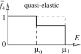
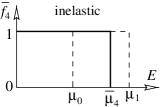
FIG. 3.: Distribution functions at the fictitious contact.

In the quasi-elastic case, the distribution function $f_{4}$ is itself a fluctuating quantity. Imposing that the contribution of the states of energy $E$ to the fluctuating part of the current at the fictitious contact is zero, $\Delta j_{4}(E)=0$, leads to a relation between the fluctuating part of the distribution $f_{4}-\bar{f}_{4}$ and the contribution of those states to the intrinsic noise $\delta j_{4}(E)$. This relation is of the same form as (8): $\Delta j_{\alpha}(E)=\delta j_{\alpha}(E)-\frac{G_{\alpha 4}}{G_{44}}\delta j_{4}(E)$.

Finally we find for the two different kinds of incoherent scattering the current correlations $S^{\rm in,qe}_{\alpha\beta}=\left\langle\Delta I_{\alpha}\Delta I_{\beta}\right\rangle$:

$$S^{\rm in,qe}_{\alpha\beta}=S_{\alpha\beta}-\frac{G_{\alpha 4}}{G_{44}}S_{\beta 4}-\frac{G_{\beta 4}}{G_{44}}S_{\alpha 4}+\frac{G_{\alpha 4}G_{\beta 4}}{G_{44}^{2}}S_{44}\>.$$ (10)

They involve the conductances $G_{\alpha\beta}$ and the intrinsic correlations $S_{\alpha\beta}=\left\langle\delta I_{\alpha}\delta I_{\beta}\right\rangle$ for the four-terminal conductor of figure 2, calculated with formula (1) where the distribution function at contact 4 is either a step like Fermi function for the potential $\bar{\mu}_{4}$ in the inelastic case (7), or the average distribution $\bar{f}_{4}$ given by (9) in the quasi-elastic case (see figure 3).

Let us now come to the results. First, for the quasi-elastic case, we find:

$$S^{\rm qe}_{23}=-\frac{e^{2}}{h}|eV|\frac{R_{3}}{4}\Big{[}2T_{3}(1+T_{1})^{2}+(1+T_{3})R_{1}^{2}\Big{]}\>.$$ (11)

In particular, in the interesting limit $T_{3}=0$ where the two edge states are perfectly separated at QPC 3, we get: $S^{\rm qe}_{23}=-\frac{e^{2}}{h}|eV|\frac{R_{1}^{2}}{4}$, i.e. half of the result (5) obtained when scattering between edge states is coherent. The auto-correlations take the values: $S^{\rm qe}_{22}=S^{\rm qe}_{33}=\frac{e^{2}}{h}|eV|\frac{R_{1}}{2}\frac{1+3T_{1}}{2}$.

More surprising is the result obtained for inelastic scattering:

$$S^{\rm in}_{23}=-\frac{e^{2}}{h}|eV|\frac{R_{3}}{2}\Big{[}2T_{3}(1+T_{1})-(1+T_{3})R_{1}T_{1}\Big{]}$$ (12)

leading to the possibility of positive correlations, as figure 4 shows (let us recall again that correlations in the presence of coherent scattering only are always negative due to the fermionic nature of carriers [23]). If $T_{3}=0$, we get $S^{\rm in}_{23}=+\frac{e^{2}}{h}|eV|\frac{R_{1}T_{1}}{2}$. This result means that this modelization of inelastic scattering gives the possibility for a fluctuation of the potential $\mu_{4}$ to inject in a correlated way in the two channels some current. Let us also mention the result for the noise in this limit: $S^{\rm in}_{22}=S^{\rm in}_{33}=\frac{e^{2}}{h}|eV|\frac{R_{1}T_{1}}{2}$.

If $T_{1}=T_{3}=0$, only one edge state is transmitted at QPC $1$, the currents in the two channels are equilibrated by inelastic processes between QPC’s, and finally the two edge states are separated by QPC 3. We remark that in this case the correlations and the noise vanish. This shows that this modelization of inelastic process does not introduce noise when it distributes the current of a noiseless channel into two channels. (This is not the case if coherent or quasi-elastic scattering occurs between edge states: $S^{\rm coh}_{23}=-\frac{e^{2}}{h}|eV|\frac{1}{2}$ and $S^{\rm qe}_{23}=-\frac{e^{2}}{h}|eV|\frac{1}{4}$).

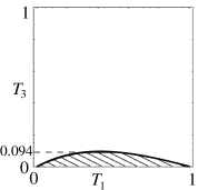
FIG. 4.: Sign of correlations $S^{\rm in}_{23}$ in the presence of inelastic scattering. The dashed area corresponds to the region in the parameter space where $S^{\rm in}_{23}>0$.

Note that if more than two edge states carry the current, still with only one partially transmitted and all others being perfectly transmitted, the region in the paramater space where the correlations are positive diminishes.

Finally we would like to discuss the effect of a finite temperature on the result (12) for $T_{3}=0$. We will show that for a high enough temperature $S^{\rm in}_{23}$ is negative. For a finite temperature $T$, the Fermi distributions at the three contacts are smoothed as well as the average distribution $\bar{f}_{4}$ at the fictitious contact. For $T_{3}=0$, equation (1) gives:

$$S^{\rm in}_{23}=\frac{e^{2}}{h}\bigg{[}-k_{B}T\left(2+{R_{1}}+{R_{1}T_{1}}\right)\hskip 56.9055pt$$ (13)

$$+\frac{R_{1}T_{1}}{2}{eV}\coth\frac{eV}{2k_{B}T}\bigg{]}\>.$$ (14)

If $T=0$ we indeed recover the positive result $S^{\rm in}_{23}=+\frac{e^{2}}{h}|eV|\frac{R_{1}T_{1}}{2}$ for the shot noise, and if $V=0$ we find $S^{\rm in}_{23}=-\frac{2e^{2}}{h}k_{B}T\left(1+\frac{R_{1}}{2}\right)$, which is the result of the fluctuation-dissipation theorem: $S^{\rm in}_{23}=2k_{B}T(G^{\rm in}_{23}+G^{\rm in}_{32})$ where $G^{\rm in}_{\alpha\beta}=G_{\alpha\beta}-\frac{G_{\alpha 4}G_{4\beta}}{G_{44}}$ is the conductance of the three-terminal conductor in the presence of incoherent scattering.

Let us define $T_{c}$, the critical temperature above which the correlations $S^{\rm in}_{23}$ are negative. For small transmission $T_{1}\ll 1$ we find: $k_{B}T_{c}\simeq|eV|\frac{T_{1}}{6}$, and for large transmission $R_{1}\ll 1$: $k_{B}T_{c}\simeq|eV|\frac{R_{1}}{4}$. The transmission that maximizes the critical temperature is $T_{1}=3-\sqrt{6}\simeq 0.55$. In this case we have: $k_{B}T_{c}^{\rm max}\simeq|eV|\frac{5\sqrt{6}-12}{2(6\sqrt{6}-12)}\simeq\frac{|eV|}{21.8}$.

IV Summary

To summarize we have shown that incoherent scattering can have a strong effect on the correlations in a HBT situation. In our modelization, inelastic scattering is responsible for positive correlations in a certain parameter range. We emphasize that the investigation of the correlations with the conductor of figure 1 for $T_{3}=0$ provides direct information about inter-edge state scattering: in the absence of inter-edge state scattering the correlation $S_{23}$ vanishes, for elastic scattering and for quasi-elastic scattering it is negative and for inelastic scattering it is positive. In principle it is possible to discriminate also between elastic inter-edge state scattering and quasi-elastic scattering: in the case of elastic scattering a single parameter ($\varepsilon$) determines the noise spectra and the conductances if $T_{1}$ and $T_{3}$ are known.

We have constructed here only the limiting case of a fictitious contact. Partially transmitting contacts would allow to interpolate between fully coherent inter-edge state scattering and fully quasi-elastic or fully inelastic inter-edge state scattering.

Acknowlegments

Interest in the topic of this work was stimulated by a question of Bart J. van Wees. We acknowledge Yaroslav M. Blanter and Andrew M. Martin for very interesting discussions. This work was supported by the Swiss National Science Foundation and by the TMR Network Dynamics of Nanostructures.

REFERENCES

- [1] M. J. M. de Jong and C. W. J. Beenakker, Physica A 230, 219 (1996).
- [2] Ya. M. Blanter and M. Büttiker, To appear in Phys. Rep., preprint cond–mat/9910158 (1999).
- [3] B. I. Halperin, Phys. Rev. B 25(4), 2185 (1982).
- [4] M. Büttiker, Phys. Rev. B 38(14), 9375 (1988).
- [5] B. J. van Wees, E. M. M. Willems, L. P. Kouwenhoven, C. J. P. M. Harmans, J. G. Williamson, C. T. Foxon, and J. Harris, Phys. Rev. B 39(11), 8066 (1989).
- [6] S. Komiyama, H. Hirai, S. Sasa, and T. Fujii, Solid State Commun. 73(2), 91 (1990).
- [7] B. W. Alphenaar, P. L. McEuen, R. G. Wheeler, and R. N. Sacks, Phys. Rev. Lett. 64(6), 677 (1990).
- [8] G. Müller, D. Weiss, A. V. Khaetskii, K. von Klitzing, S. Koch, H. Nickel, W. Schlapp, and R. Lösch, Phys. Rev. B 45(7), 3932 (1992).
- [9] M. Henny, S. Oberholzer, C. Strunk, T. Heinzel, K. Ensslin, M. Holland, and C. Schönenberger, Science 284, 296 (1999).
- [10] S. Oberholzer, M. Henny, C. Strunk, C. Schönenberger, T. Heinzel, K. Ensslin, and M. Holland, Physica E 6, 314 (2000).
- [11] M. Büttiker, Phys. Rev. Lett. 65(23), 2901 (1990).
- [12] T. Martin and R. Landauer, Phys. Rev. B 45(4), 1742 (1992).
- [13] W. D. Oliver, J. Kim, R. C. Liu, and Y. Yamamoto, Science 284, 299 (1999).
- [14] M. T. Woodside, C. Vale, P. McEuen, C. Kadow, K. Maranowski, and A. C. Gossard, preprint cond–mat/0002391 (2000).
- [15] M. Büttiker, Phys. Rev. B 33(5), 3020 (1986).
- [16] C. W. J. Beenakker and M. Büttiker, Phys. Rev. B 46(3), 1889 (1992).
- [17] S. A. van Langen and M. Büttiker, Phys. Rev. B 56(4), R1680 (1997).
- [18] J. D’Amato and H. M. Pastawski, Phys. Rev. B 41(11), 7411 (1990).
- [19] T. Ando, Surf. Sci. 361/362, 270 (1996).
- [20] F. Gagel and K. Maschke, Phys. Rev. B 54(19), 13885 (1996).
- [21] N. A. Mortensen, A.-P. Jauho, and K. Flensberg, preprint , cond–mat/9909029 (1999).
- [22] M. T. Liu and C. S. Chu, Phys. Rev. B 61(11), 7645 (2000).
- [23] M. Büttiker, Phys. Rev. B 46(19), 12485 (1992).
- [24] T. Ohtsuki and Y. Ono, J. Phys. Soc. Jpn. 58, 3863 (1989).
- [25] T. Martin and S. Feng, Phys. Rev. B 64(16), 1971 (1990).