Bose condensates at high angular momenta

Abstract

We exploit the analogy with the Quantum Hall (QH) system to study weakly interacting bosons in a harmonic trap. For a $\delta$-function interaction potential the “yrast” states with $L\geq N(N-1)$ are degenerate, and we show how this can be understood in terms of Haldane exclusion statistics. We present spectra for 4 and 8 particles obtained by numerical and algebraic methods, and demonstrate how a more general hard-core potential lifts the degeneracies on the yrast line. The exact wavefunctions for $N=4$ are compared with trial states constructed from composite fermions (CF), and the possibility of using CF-states to study the low $L$ region at high $N$ is discussed.
PACS numbers: 03.75.Fi, 05.30.Jp, 73.40.Hm

The close relation between high angular momentum states of a condensate of weakly interacting hard core bosons [1, 2, 3] and the Quantum Hall (QH) effect was recently pointed out [4, 5, 6]. The essential observation is that the weak interaction limit allows for a two-dimensional description of the boson system in terms of lowest Landau level (LLL) wave functions [4] – just as for a QH system, and they are both described by wave functions containing powers of the Laughlin-Jastrow factor $\prod_{i<j}(z_{i}-z_{j})$, where $z_{i}$ is the complex coordinate of the $i^{th}$ particle. As pointed out by Cooper and Wilkin [6], the two systems can in fact be mapped onto each other by a standard Leinaas-Myrheim transformation [7], attaching an odd number of units of statistical flux to each particle. This enables us to use both intuition and techniques from the QH system to study rotating Bose condensates. In this paper we shall mainly discuss the angular momentum region $N(N-1)\leq L\leq 2N(N-1)$, where the ground state corresponding to a $\delta$-function two-body interaction is degenerate. We explicitly show how these degeneracies can be understood via a mapping to a system of free anyons in the LLL, and then show how the degeneracy is broken by a more general short range potential containing derivatives of delta functions. We also make a detailed comparison between algebraically calculated exact wave functions and trial wave functions formed from so called compact states of composite fermions, a construction orginally due to Jain and Kawamura [8]. In particular, we will emphasize the importance of a certain class of wavefunctions where the polynomial part is translationally invariant.
Although for computational reasons we have results only for few particles, $N=4,6$ and 8, it is clear that some of our results, like the degeneracy structure of the yrast line, hold for any $N$. We also believe that many features of the results for the CF wave functions will generalize to higher $N$ .
Since the flux attachment changes the angular momentum by $mN(N-1)/2$, where $m$ is the number of fluxes attached, the boson - fermion mapping would apparently only be useful for studying angular momenta that are out of reach of present experiments[9] (which are limited to the strong interaction regime and $L\sim N$). However, there are some indications that fermionic techniqes could be useful for $L$ as low as $N$, i.e. for the so called single vortex state. Although we will return to this point at the end of the paper, we shall for now, without any further apologies, consider the theoretical problem of understanding the region $N(N-1)\leq L\leq 2N(N-1)$ of the yrast line.

The simplest model for a hard-core interaction is a delta function potential. We thus consider a model of $N$ interacting spinless bosons in a harmonic trap of strength $\omega$. In the limit of weak interaction, this may be rewritten [4] as a two-dimensional lowest Landau level (LLL) problem in the effective “magnetic” field $B_{eff}=2m\omega$ with the Hamiltonian taking the form

$$\mbox{$$}H=\omega L+g\sum_{i<j}\delta^{2}({\bf r}_{i}-{\bf r}_{j})\$$ (1)

($\hbar=1$), where $L\equiv\sum_{i}l_{i}=L_{z}$ is the total angular momentum. The single-particle states spanning our Hilbert space are $\eta_{0,l}=(2^{l+1}\pi l!)^{-1/2}z^{l}\exp(-\bar{z}z/4)$ with $z=\sqrt{2m\omega}(x+iy)$.

In Figs. 1 and 2 we show the interaction energy, in units of $g/4\pi$ as a function of the total angular momentum $L$ for $N=4$, $L\leq 20$ and $N=8$, $30\leq L\leq 56$, respectively. The many-body states are obtained from Lanczos diagonalization suitable for large and relatively sparse matrices [10]. The Fock space is spanned by single-particle states that are characterized only by the positive quantum numbers $l$, where $0\leq l\leq L$. (Similar exact diagonalization studies have recently been reported in [6] and [11].) We note the following properties in the many-body spectra: Since increasing the angular momentum spreads out the particles in space, the yrast energy, i.e. the lowest possible interaction energy for given $L$, decreases with increasing $L$. For each state in the spectrum, there exists a set of “daughter states” with higher values of $L$, having exactly the same (interaction) energy as the original state. These daughters are simply center-of-mass excitations of the original states, thus having the same many-body correlations[12].

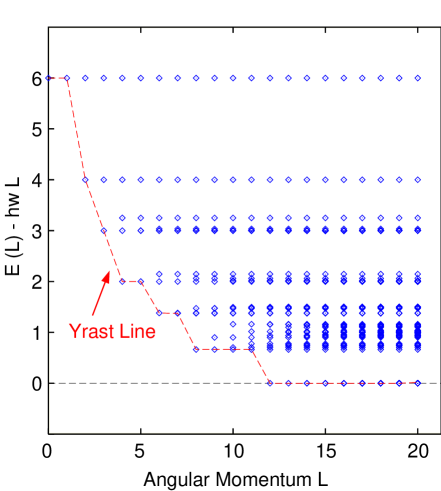
FIG. 1.: Many-body spectra of $N=4$ weakly interacting bosons in a harmonic trap for $L\leq 20$. The dashed line connects the yrast states

FIG. 2.: As Fig. 1, but for $N=8$ and $30\leq L\leq 56$, showing only the 100 lowest eigenvalues

For $L\geq N(N-1)$ there are zero energy states, which can be understood by noting that any wavefunction of the form

$$\mbox{$$}\psi(z_{1},z_{2},...,z_{N})=\prod_{i<j}(z_{i}-z_{j})^{2}S(z_{1},z_{2},...,z_{N})\ \ \ ,$$ (2)

where $S(z_{1},z_{2},...,z_{N})$ is a symmetric polynomial in the $z_{i}$:s, has zero interaction energy. Since the factor $\prod_{i<j}(z_{i}-z_{j})^{2}$ contributes an angular momentum $L_{0}=N(N-1)$, states of the type (2) exist for $L\geq L_{0}$.

At $L=N(N-1)$ there is a unique state with zero interaction energy corresponding to $S(z_{1},z_{2},...,z_{N})=1$, while the states at higher $L$ typically are degenerate. The systematics of these degeneracies can be understood by a mapping to anyons in the lowest Landau level. The essential observation is that the wave functions (2) describe anyons in the LLL with statistics parameter $\alpha=2$[13] (in general, the statistics parameter is given by the exponent of the Jastrow factor). It is known[13, 14, 15] that anyons in the LLL obey Haldane’s fractional exclusion statistics (FES)[16], and following Ref.[13], one can use this knowledge to construct the allowed many-body states for given $N$ and $L$ as angular momentum excitations of the Laughlin-like state at $L=N(N-1)$. According to the definition of FES, each particle in the system blocks $\alpha=2$ single-particle states, and many-particle states with total angular momentum $L$ are constructed by occupying single-particle states, with a minimum distance of $\alpha=2$ between each pair of occupied levels (for an example, see Fig. 3). The number of allowed configurations then gives the degeneracy of the state for a given $L$.

FIG. 3.: FES construction of yrast states for $N=4$, $L=12(=L_{0})$, 13 and 14. The $L=12$ and $L=13$ states are non-degenerate, whereas $L=14$ has degeneracy 2.

Table 1 shows the degeneracies of some of the states on the $N=4$ yrast line, as obtained from the anyon mapping, and they are in exact agreement with our numerical results.

$L$	12	13	14	15	16	17	18	19	20
$d$	1	1	2	3	5	6	9	11	15

TABLE I.: Degeneracy $d$ of the lowest $L$-excitations above the Laughlin state for $N=4$.

This construction implicitly uses that all the eigenstates on the yrast line for $L>N(N-1)$ contain the Jastrow factor $\prod_{i<j}(z_{i}-z_{j})^{2}$, so the degeneracies can also be found as the number of ways one can distribute $M=L-L_{0}$ units of angular momentum among $N$ particles.

For a more general hard core potential, the $E=0$ states on the yrast line above $L=N(N-1)$ are no longer degenerate. To demonstrate this point and study how the degeneracy is broken, we add a potential of the form

$$\mbox{$$}V=c_{1}\nabla^{2}\delta^{2}(z-z^{\prime})+c_{2}\nabla^{4}\delta^{2}(z-z^{\prime}),$$ (3)

that was originally used by Trugman and Kivelson[12] in the context of the fractional QH effect. The term $\sim\nabla^{2}\delta^{2}(z-z^{\prime})$ does not contribute to the interaction energy for fully symmetric states, whereas the $\nabla^{4}\delta^{2}(z-z^{\prime})$ term gives small corrections to the spectra in Figs. 1 and 2 (at the percent level for the parameters used in the inset of Fig. 4, where we show regularized forms of the potentials (1) and (3)).

We have examined how the potential (3) splits up the degeneracies of the zero interaction energy yrast states, by exact algebraic diagonalization, using computer algebra. Here we have directly used the form (2), and systematically exploited that for a given $L$, all states corresponding to center-of-mass excitations of lower $L$-eigenstates are orthogonal to the subspace of “new” states. The latter subspace consists of translation invariant (TI) polynomials, i.e. functions invariant under a simultaneous, constant shift $z_{i}\rightarrow z_{i}+a$ of all the coordinates[12]. Following Trugman and Kivelson[12], we have used a basis constructed from elementary symmetric functions $s_{n}$. For given $N$ and $L$, the basis consists of all possible combinations

$$\mbox{$$}|k_{1}k_{2}...k_{n}\rangle\equiv s_{1}^{k_{1}}(z_{i})s_{2}^{k_{2}}(\tilde{z}_{i})...s_{N}^{k_{N}}(\tilde{z}_{N})\,\prod_{i<j}(z_{i}-z_{j})^{2},$$ (4)

such that $\sum_{n=1}^{N}nk_{n}=L-L_{0}$. Note that, for $n\geq 2$, we have introduced the new variables $\tilde{z}_{i}\equiv z_{i}-z_{c}$, with $z_{c}$ the center-of-mass coordinate $z_{c}=(\sum z_{i})/N$. The basis states spanning the TI subspace are identified as those with $k_{1}=0$. The diagonalization is thus performed within this subspace only, which reduces the matrix dimension substantially. The resulting spectrum for $N=4$, with the coefficient $c_{2}$ in (3) set equal to 1, is shown in Fig. 4. We notice the close similarity between Fig. 1 and 4. In both cases, the yrast line passes through the same number of steps, with the same step lengths, as $L$ is increased by $N(N-1)$, to the point where the yrast energy becomes zero. At the point $L=2N(N-1)$, the zero-energy yrast state is again non-degenerate and of the Laughlin type, i.e. $\prod_{i<j}(z_{i}-z_{j})^{4}$, whereas the subsequent yrast states have degeneracies corresponding to FES with statistics parameter $\alpha=4$. Including even higher derivative terms in the repulsive potential would subsequently split up the higher regions of the yrast line. Finally, note that the yrast states corresponding to cusps, i.e. states that are followed by a “plateau” in the yrast line, are always in the TI subspace.

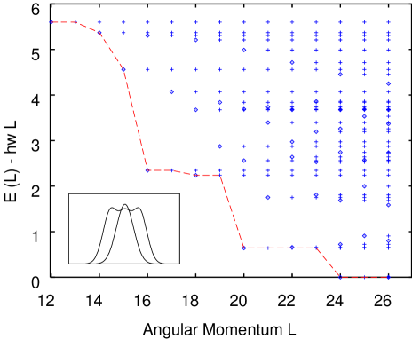
FIG. 4.: Yrast spectrum for $N=4$ and $12\leq L\leq 26$, for a repulsive potential $\nabla^{4}\delta^{2}(z-z^{\prime})$. Translation invariant eigenstates are denoted by diamonds, whereas the crosses denote center-of-mass excitations. Inset: Delta function potential (regularized as a gaussian) and a potential including the terms (3), with $c_{1}=0.023$ and $c_{2}=0.00008$. We see that the latter more closely resembles a hard sphere potential.

The algebraic diagonalization used here is limited in practice to smaller particle numbers and angular momenta than the numerical scheme used in Figs. 1 and 2. However, the present approach has the advantage that it provides explicit, analytic expressions for the eigenfunctions, in terms of symmetric polynomials. This gives some additional insight into the structure of the yrast states, and in particular the region below the single vortex in the case of a pure delta function interaction. Bertsch and Papenbrock [11] recently proposed and numerically tested the following form for the yrast states at $2\leq L\leq N$,

$$\mbox{$$}\psi_{L}(z_{i}) = \sum_{p_{1}<p_{2}<...<p_{L}}(z_{p_{1}}-z_{c})(z_{p_{2}}-z_{c})...(z_{p_{L}}-z_{c})\ .$$ (5)

This is just the symmetric polynomial $s_{L}(\tilde{z}_{i})$, i.e. the state $|0...1..0\rangle$ (with the 1 in the $L$th place), in the notation of (4) (without the Jastrow factor in the present case of a pure delta function interaction). This state is a basis state in the TI subspace for all $2\leq L\leq N$. In the cases where this is the only basis state ($L=2,3$ for $N\geq 3$), it is thus obvious that (5) is exact. Furthermore, performing the algebraic diagonalization up to $L=N$ for $N=4$ and $N=6$, we have confirmed that even when the translation invariant subspace is spanned by more than one basis vector, the basis state (5) is always an exact eigenstate.

We now turn to a study of a class of wave functions that can be constructed in analogy with the so-called Jain states for the fractional QHE[17]. The main idea is to map the strongly interacting LLL bosons to weakly interacting composite fermions by attaching an odd number $m$ of flux quanta to each particle. Trial wavefunctions with angular momentum $L$ are thus constructed as non-interacting fermionic wavefunctions with angular momentum $L-m/2\,N(N-1)$, multiplied by $m$ Jastrow factors and projected onto the LLL,

$$\mbox{$$}\psi_{L}={\cal P}\left(f_{F}(z_{i},\bar{z}_{i})\,\prod_{i<j}(z_{i}-z_{j})^{m}\right)\ \ \ \ .$$ (6)

Here, $f_{F}$ is a Slater determinant consisting of single-particle wave functions $\eta_{n,l}(z,\bar{z})\propto z^{l}L_{n}^{l}(\bar{z}z/2)$ where $n$ is the Landau level index ( $l\geq-n$), and $L_{n}^{l}$ a generalized Laguerre polynomial.

Originally used for the homogeneous states relevant for the fractional QHE, wavefunctions of the type (6) were later employed to describe inhomogeneous systems such as quantum dots[8, 18, 19] and recently by Cooper and Wilkin [6] to study the bosonic yrast lines for up to 10 particles in the case of a pure delta function interaction.

In short, the LLL projection in (6) amounts to the replacement $\bar{z}_{i}\rightarrow 2\partial_{i}$ in the polynomial part of the wave function. However, there are several ways of doing this in practice, and we shall compare the different projection methods when constructing trial wave functions for the yrast states in Figs. 1 and 4. The most straightforward way is to replace the $\bar{z}$:s with derivatives in the final polynomial, obtained after multiplying out the Slater determinant and the Jastrow factors and moving all $\bar{z}$:s to the left. In practice, this method is applicable only for small particle numbers, when the number of derivatives involved is not too large. We shall refer to this method as “Method I” and apply it in a few special cases for comparison.

Alternatively, noting that[17]

$$\mbox{$$}\left|\begin{array}[]{ccc}\eta_{11}&\eta_{12}&..\\ \eta_{21}&\eta_{22}&..\\ ...&...&..\\ \eta_{N1}&\eta_{N2}&..\end{array}\right|\prod_{i<j}(z_{i}-z_{j})^{2p}=\left|\begin{array}[]{ccc}\tilde{\eta}_{11}&\tilde{\eta}_{12}&..\\ \tilde{\eta}_{21}&\tilde{\eta}_{22}&..\\ ...&...&..\\ \tilde{\eta}_{N1}&\tilde{\eta}_{N2}&..\end{array}\right|,$$ (15)

where $\eta_{ij}\equiv\eta_{i}(z_{j},\bar{z}_{j})$ and $\tilde{\eta}_{ij}\equiv\eta_{i}(z_{j},\bar{z}_{j})\prod_{k\neq j}(z_{j}-z_{k})^{p}$, one can first absorb $2p$ Jastrow factors in the Slater determinant, and then project entry by entry. Since the wave function (6) contains an odd number $m$ of Jastrow factors, one finally has to compensate by multiplying the resulting polynomial by $\prod_{i<j}(z_{i}-z_{j})^{m-2p}$. We shall refer to this as Method II and use it as follows; for a delta function interaction, where the wave function contains $m=1$ Jastrow factor, it is appropriate to use $p=1$ (Method IIa). In the case of the $\nabla^{4}\delta$-potential, the Jain construction will involve absorbing $m=3$ flux quanta in the wave function, and we shall compare projection with $p=1$ (Method IIa) and $p=2$ (Method IIb). (Note that Method IIa is in a sense trivial, since it relates the wavefunctions at $L$ and $L+N(N-1)$ by multiplication with two Jastrow factors.)

We have already stressed the significance of the TI subspace - these are the states that determine the shape of the yrast line. It is very appealing that there is a special set of the states (6) that are in this subspace, namely the so called compact states [8] which are characterized by having the $n$:th Landau level occupied from $l_{n}=-n$ to $l_{n}=l_{n}^{max}$ without any “holes”. In the context of the QH effect, the important property of the compact states is that they are homogeneous. When describing quantum dots using the non-interacting composite fermion model (NICFM), one can show that CF candidates for the cusp states must be compact[8], and the same line of arguments was later used for bosons [18, 6]. From the point of view of the wavefunctions, the importance of the compact states is that they are in the TI subspace, and it is rather remarkable that for all L where a compact state can be constructed, the one with the lowest CF energy has a large overlap with the lowest exact state in the TI subspace. This is true, independent of whether or not the state is a ground state, i.e. corresponds to a cusp in the yrast line. In the following discussion, we shall only be concerned with the wavefunctions, and will not discuss whether or not the NICFM can give a good description of the energy spectrum, a question that was already discussed in some detail [8, 18, 19].

$\delta$-function potential: In this case we have calculated the Jain wavefunctions (6) corresponding to all compact states for $N=4$, $0\leq L\leq 12$, taking $m=1$ and using projection method IIa ($p=1$). If there are two compact states with the same $L$, we use the one with the lowest CF effective energy. In table II we show the overlap with the exact algebraic wavefunctions. A “1” indicates that the wavefunctions are identical. For comparison we have also included the overlaps with the wavefunctions corresponding to projection method I, as given by Cooper and Wilkin[6]. We note that all the compact states have very large overlap with the exact eigenstates. That the CF wavefunction is exact for $L=2,3$ is a simple consequence of the TI property and that there is only one state in the TI subspace at these $L$ values. That the $L=7$ state comes out exact is more surprising, and we have no good explanation for this. It would be interesting to pursue the exact diagonalization to higher $N$ in order to see if there are other non-trivial CF states that are exact. We also note that the direct projection (method I) does slightly better than method II.

$L$	0	2	3	4	6	7	8	12
${\rm IIa}$	1	1	1	0.944	0.962	1	0.997	1
${\rm I}$	1			0.980	0.980		0.997	1

TABLE II.: Overlaps between trial and exact wave yrast functions for $N=4$, $0\leq L\leq 12$ and a pure delta function interaction, using projection methods IIa and I (see text).

$\nabla^{4}\delta$-function potential: Here we calculated the Jain wavefunctions (6) corresponding to all, lowest CF-energy, compact states for $N=4$, $12\leq L\leq 24$ taking $m=3$ and using projection methods IIa ($p=1$) and IIb $(p=2$). For comparison, we also used method I for three $L$ values. In table III we show the overlap with the exact algebraic wavefunctions. We again note that all the compact states (except $L=17$ with projection method I) have very large overlap with the exact eigenstates, and that for $L=17,19$, the CF state is not the ground state. Comparing the different projection methods, we see that in many, but not all cases they give identical results. In particular, one should note that method IIb does not reproduce the exact wavefunction for $L=14,15$ where the TI subspace is non-degenerate. This means that that projection gives a wave function that is not in the space of states given by (2). The same effect is even more striking for $L=17$, where method IIb gives the exact wave function, whereas direct projection (method I) gives a rather poor overlap, indicating that a large component is not in the subspace (2).

$L$	12	14	15	16	$17^{*}$	18	$19^{*}$	20	24
${\rm IIa}$	1	1	1	0.988		0.910	0.993	0.986	1
${\rm IIb}$	0.938	0.910	0.988	0.990	1	0.910	0.993	0.986	1
${\rm I}$					0.591		0.993	0.986	1

TABLE III.: Overlaps between trial and exact yrast wave functions for $N=4$, $12\leq L\leq 24$, using two different projection methods (see text). The asterisk indicates that the $L=17$ and $L=19$ Jain states (which correspond to the lowest TI states) are not yrast states, but lie higher in energy than the CM excitation of the previous $L$ state. Note that projection method IIa gives zero for $L=17$.

Finally, we comment on the possibility to use CF wavefunctions in the experimentally more relevant case of low $L$, and in particular for the single vortex state at $L=N$. Rather surprisingly, the overlaps between the CF and the exact wavefunction (5) tend to get larger with increasing particle number, at least up to $N=10$.[6] It thus seems worthwhile to use the CF approach to construct trial wavefunctions for the single vortex for general $N$. The single vortex CF state is in fact unique, if one demands that in addition to being compact, it should also have minimal CF cyclotron energy. The relevant Slater determinant is formed from the single particle states $\eta_{n,-n}$ for $n=N-2,N-1,...0$ and $\eta_{01}$, and, using projection method I, the resulting wavefunction takes the following rather compact form,

$$\mbox{$$}\psi_{L=N}=\sum_{n=1}^{N}(-1)^{n}z_{n}\prod_{k<l;k,l\neq n}\left(\partial_{k}-\partial_{l}\right)\prod_{i<j}(z_{i}-z_{j}).$$ (16)

Although the $\sim N^{2}$ derivatives make it difficult to evaluate this function for large $N$, it can easily be handled in integrals of the form $\int\prod_{i}d^{2}z_{i}\,\exp(-1/2\sum_{i}\bar{z}_{i}z_{i})f(\bar{z}_{i})\psi_{L=N}$ by partial integrations. Alternatively one can use projection Method II, where the wavefunction becomes a determinant of linear combinations of elementary symmetric polynomials. In both cases, it should be possible to compare with the exact wavefunction (5) using Monte Carlo methods.

ACKNOWLEDGEMENT: We are very grateful to B. Mottelson for introducing us to the physics of rotating Bose condensates, and for numerous fruitful discussions. We also wish to thank M. Manninen, G. Kavoulakis and R.K. Bhaduri for discussions and M. Koskinen for giving advice on the numerical work. This work was financially supported by the Academy of Finland, the Swedish Natural Science Research Council, the TMR programme of the European Community under contract ERBFMBICT972405, the “Bayerische Staatsministerium für Wissenschaft, Forschung und Kunst”, and the NORDITA Nordic project “Confined electronic systems”.

REFERENCES

- [1] D. A. Butts and D. S. Rokhsar, Nature 397, 327 (1999).
- [2] B. Mottelson, Phys. Rev. Lett. 83, 2695 (1999).
- [3] G. M. Kavoulakis, B. Mottelson and C. J. Pethick, to be published.
- [4] N. K. Wilkin, J. M. F. Gunn and R. A. Smith, Phys. Rev. Lett. 80, 2265 (1998).
- [5] N. K. Wilkin and J. M. F. Gunn, Phys. Rev. Lett. 84, 6 (2000).
- [6] N. R. Cooper and N. R. Wilkin, Phys. Rev. B 60, R16279 (1999).
- [7] J. M. Leinaas and J. Myrheim, Nuovo Cimento 37 B, 1 (1977).
- [8] J. K. Jain and T. Kawamura, Europhys. Lett. 29, 321 (1995).
- [9] M. R. Matthews et al. , Phys. Rev. Lett. 83, 2498 (1999); K. W. Madison, F. Chevy, W. Wohlleben and J. Dalibard, cond-mat/9912015.
- [10] R. B. Lehoucq, D.C. Sørensen and Y. Yang, ARPACK User’s guide: Solution to large scale eigenvalue problems with implicitly restarted Arnoldi methods. See http://www.caam.rice.edu/software/ARPACK
- [11] G. F. Bertsch and T. Papenbrock, Phys. Rev. Lett. 83, 5412 (1999).
- [12] S. A. Trugman and S. Kivelson, Phys. Rev. B 31, 5280 (1985).
- [13] T. H. Hansson, J. M. Leinaas and S. Viefers, Nucl. Phys. B 470[FS], 291 (1996).
- [14] S. B. Isakov and S. Viefers, Int. J. Mod. Phys. A 12, 1895 (1997).
- [15] A. Dasnières de Veigy and S. Ouvry, Phys. Rev. Lett. 72, 600 (1994); Y. S. Wu, Phys. Rev. Lett. 73, 922 (1994); D. Li and S. Ouvry, Nucl. Phys. B 430, 563 (1994).
- [16] F. D. M. Haldane, Phys. Rev. Lett. 67, 937 (1991).
- [17] For a review, see J. K. Jain and R. K. Kamilla in Composite Fermions: A unified view of the quantum Hall effect, ed. O. Heinonen (World Scientific, River Edge, N.J., 1998).
- [18] B. Rejaei, Phys. Rev. B 48, 18016 (1993).
- [19] C. W. J. Beenakker and B. Rejaei, Physica B 189, 147 (1993).