RVB description of the low-energy singlets of the spin 1/2 kagomé antiferromagnet

Abstract

Extensive calculations in the short-range RVB (Resonating valence bond) subspace on both the trimerized and the regular (non-trimerized) Heisenberg model on the kagomé lattice show that short-range dimer singlets capture the specific low-energy features of both models. In the trimerized case the singlet spectrum splits into bands in which the average number of dimers lying on one type of bonds is fixed. These results are in good agreement with the mean field solution of an effective model recently introduced. For the regular model one gets a continuous, gapless spectrum, in qualitative agreement with exact diagonalization results.

1 Introduction

It is well known that the conventional picture of a long-range, ordered, dressed Néel ground state (GS) can collapse for low dimensional frustrated antiferromagnets. The GS of several spin 1/2 strongly frustrated systems has no long range antiferromagnetic order and is separated from the first magnetic ($S=1$) excitations by a gap. The first example of such a behavior was given by the zigzag chain at the Majumdar-Ghosh point Majumdar ($J_{2}/J_{1}=1/2$) in which case the two-fold degenerate GS is a product of singlets built on the strong bonds.

In some cases the consequences of frustration on the structure of the spectrum can be even more dramatic. It is now firmly established by many numerical studies that the singlet-triplet gap of the Heisenberg model on the kagomé lattice is filled with an exponential number of singlet states Waldtmann . This property is actually not specific to the kagomé antiferromagnet (KAF) and could be a generic feature of strongly frustrated magnets: It is suspected to occur also for the Heisenberg model on the pyrochlore lattice Canalspriv , and it has been explicitly proved for a one-dimensional system of coupled tetrahedra which can be seen as a 1D analog of pyrochlore Mambrini .

Since the particular low-temperature dependence of many physical quantities is directly connected to the structure of this non-magnetic part of the spectrum, many recent works Waldtmann ; Zengelser1 ; Singhhuse ; Leungelser ; Zengelser2 ; Sindzingre ; Nakamura ; Lecheminant were devoted to understand the nature of the disordered GS and low-lying excitations. Unfortunately, it is still hard to come up with a clear picture of the low-energy sector of the KAF. Resonating Valence Bonds (RVB) states, for which wave functions are products of pair singlets, seem to be a natural framework to describe this exponential proliferation of singlet states. RVB states were first proposed to describe a disordered spin liquid phase by Fazekas and Anderson Fazekas for the triangular lattice and was reintroduced by Anderson Anderson in the context of high-$T_{c}$ superconductivity.

For the kagomé lattice, the absence of long range correlation may lead to consider only Short Range RVB states (SRRVB) , i.e. first neighbor coverings of the lattice with dimers. The first difficulty which occurs is that the number of SRRVB states of a $N$ site kagomé lattice with periodic boundary conditions is $2^{1+(N/3)}\sim 2(1.26)^{N}$ Elser whereas the number of singlet states before the first triplet of the KAF scales like $1.15^{N}$ Waldtmann . Of course, this does not necessarily disqualify the SRRVB description but raises the question of the selection of the relevant states.

At the mean field level an answer to this question has been given in a recent paper Mila starting from a trimerized remark version of the KAF (see Fig. 1):

$${\cal H}=J_{\triangledown}\sum_{\langle i,j\rangle_{\triangledown}}\vec{S}_{i}.\vec{S}_{j}+J_{\vartriangle}\sum_{\langle i,j\rangle_{\vartriangle}}\vec{S}_{i}.\vec{S}_{j},$$ (1)

Figure 1: Trimerized kagomé lattice: strong bond triangles form a (N/3) site triangular lattice.

When considering low-energy excitations one can work in the subspace where the total spin of each strong bond triangle is $1/2$. Since there are two ways to build a spin $1/2$ with three spins $1/2$, these triangles have two spin $1/2$-like degrees of freedom : The total spin $\vec{\sigma}$, and the chirality $\vec{\tau}$. This representation does not simplify the problem because spin and chirality are coupled in the Hamiltonian but it is no longer the case in the mean field approximation and it is possible to solve the mean-field equations exactly Mila . Low-energy states are SRRVB states on the triangular lattice formed by strong bond triangles and their number grows like the number of dimer coverings of a $N/3$ site triangular lattice, $1.15^{N}$, as can be shown using standard methods Fisher ; Kasteleyn .

This result was established under the assumptions that $J_{\triangledown}/J_{\vartriangle}$ is small (trimerized limit) and that quantum fluctuations can be treated at the lowest order (mean field approximation). Therefore two questions remain open: What happens beyond mean field approximation ? Can SRRVB state give a good description of the energy spectrum in the isotropic limit?

To answer these questions we have studied the KAF Hamiltonian in the subspace of SRRVB states with no simplifying approximation concerning the non orthogonality of this basis. In this subspace the complete spectrum is obtained up to 36-site clusters in both trimerized and isotropic limit.

The text is organized as follows: In the first part we study the trimerized model and show that mean field predictions are robust with respect to quantum fluctuations. In the trimerized limit, the low-energy spectrum splits into bands in which the average number of dimers lying on one type of bonds is fixed and the size of the lowest band scales as $1.15^{N}$.

Next we present the results obtained in the isotropic limit. Contrary to what was suggested by previous studies Zengelser2 the singlet spectrum obtained with SRRVB states is a continuum. Moreover the number of states below a given total energy increases exponentially for all energy with the size of the system considered.

Finally, we compare the results obtained for KAF with the results obtained using the same basis for a non-frustrated antiferromagnet, the Heisenberg model on a square lattice, and we emphasize the ability of SRRVB states to capture the specific low energy physics of frustrated magnets.

Most of the results presented here contrast with the commonly admitted point of view that SRRVB states do not provide a good variational basis for this problem. In fact, SRRVB states lead to specific numerical difficulties due to the fact that they are not orthogonal to each other. A way to get around this difficulty is to neglect overlap between states under a given threshold. However reasonable this approximation may seem, it appears to modify the results significantly. It turns out that this approximation is not necessary to perform exact numerical simulations, even for large systems. In order to clarify this point, some technical details about the method we used to implement symmetries of the problem and achieve the calculations in this non-orthogonal basis are given in an Appendix.

2 The trimerized model

As stated in the introduction, the main question with the trimerized model ($J_{\triangledown}/J_{\vartriangle}<1$) is to know if the mean-field selection mechanism (pairing of strong bond triangles) of low-lying singlet states is robust when quantum fluctuations are taken into account.

Fully trimerized limit – Ground state. Let us start with the limit $J_{\triangledown}/J_{\vartriangle}=0$. In this limit the system consists of $N/3$ independent triangles and the SRRVB GS is obtained by putting one dimer on each of these triangles. Since $J_{\triangledown}/J_{\vartriangle}=0$ this state can be completed to a SRRVB state ($N/2$ dimers) by putting the $N/6$ remaining dimer on the $J_{\triangledown}$ bonds. The energy of such a state is $-(3/4)J_{\vartriangle}(N/3)=-(N/4)J_{\vartriangle}$. In this limit the GS is thus obtained by maximizing the number of dimers on the $J_{\vartriangle}$ bonds ($N/3$).

Figure 2: Typical dimer covering of the lattice with $n_{\text{def}}(J_{\vartriangle})=1$ (defaults are marked with a star).

By a simple counting argument it is easy to see that every SRRVB state contains $N/6=N_{t}/4$ triangles, called defaults, for which none of the bonds is occupied by a dimer ($N_{t}=(2N/3)$ is the number of triangles): a SRRVB state being a set of $N/2$ dimer, it leaves $(2N/3)-(N/2)=(N/6)$ triangles unoccupied. The number of defaults $n_{\text{def}}(J_{\vartriangle})$ on the $J_{\vartriangle}$ bonds can take all the values from $0$ to $N/6$. In terms of defaults the GS discussed above is a SRRVB state which minimizes $n_{\text{def}}(J_{\vartriangle})$.

Let us turn to the question of the degeneracy of this GS and show that the number of dimer coverings of the kagomé lattice with $n_{\text{def}}(J_{\vartriangle})=0$ is exactly the number of dimer coverings of the $N/3$ site triangular lattice formed by $\vartriangle$ triangles. To prove this, we have to check that one can associate each GS configuration to a unique dimer covering of the triangular super-lattice and vice versa (see Fig. 3).

Clearly, to each pairing $A$ of $\vartriangle$ triangles one can associate a set of dimers $(1,2,3)$ on the kagomé lattice. Doing so, the number of dimers on $\vartriangle$ triangles is $N/3$, which is the maximum, and $n_{\text{def}}(J_{\vartriangle})=0$. Consider now a SRRVB with $n_{\text{def}}(J_{\vartriangle})=0$. Let us show that there exists a unique way to pair $\vartriangle$ triangles according to the $(1,2,3)$ pattern. Starting from dimer $1$ on triangle $T1$, the existence of dimer $2$ is necessary because the state is SRRVB and the triangle $T2$ contains dimer $3$ because there is no default on $\vartriangle$ triangles by assumption.

Figure 3: The number of coverings with dimers (A) of the $N/3$ site triangular lattice of strong bond triangles is equal to the number of covering of the original lattice which satisfy $n_{\text{def}}(J_{\vartriangle})=0$ (sets of $(1,2,3)$ dimer patterns).

For the triangular lattice, the number of coverings increases with the number of sites $N$ like $A\alpha_{\text{t}}^{N}$ with $\alpha_{t}=\exp\{\frac{1}{16\pi^{2}}\int_{0}^{2\pi}\int_{0}^{2\pi}\ln(4+4\sin x\sin y+4\sin^{2}y)dxdy\}\simeq 1.5351$ and $A\simeq 2$ Mila . Thus the number of dimer coverings of the kagomé lattice with $n_{\text{def}}(J_{\vartriangle})=0$ increases like $(\alpha_{\text{t}}^{1/3})^{N}\sim 1.1536^{N}$.

This degeneracy has been obtained considering only SRRVB subspace. In the full $S=0$ subspace the GS is much more degenerate. The model, when $J_{\triangledown}/J_{\vartriangle}=0$, simply reads:

$${\cal H}=(J_{\vartriangle}/2)\sum_{i}\left\{S_{\vartriangle_{i}}(S_{\vartriangle_{i}}+1)-(9/4)\right\},$$ (2)

where $S_{\vartriangle_{i}}$ is the total spin of the triangle $i$.

The GS is thus obtained by setting the total spin of each $\vartriangle$ triangle to $1/2$ and to couple all the $N/3$ spin $1/2$ triangles to a total spin of $0$ and the degeneracy is $2^{N/3}\;(N/3)!/[(N/6)!(1+N/6)!]$. The combinatory factor is the size of the singlet sector of $N/3$ spin $1/2$ and the other factor refers to the fact that on each of the $\vartriangle$ triangles there are 2 independent ways to build a total spin of $1/2$.

Thus asymptotically the full singlet degeneracy increases like $2^{2N/3}/N^{3/2}\sim 1.5874^{N}/N^{3/2}$. The table 1 summarizes the various degeneracies.

# of sites	12	24	36	$\bf N$
S=0	132	$2.1\;10^{5}$	$4.8\;10^{8}$	$\sim\frac{2^{N}}{N^{3/2}}$
GS deg. (S=0)	32	3584	$5.4\;10^{5}$	$\sim\frac{1.5874^{N}}{N^{3/2}}$
SRRVB	32	512	8192	$\sim 1.26^{N}$
GS deg. (SRRVB)	12	72	348	$\sim 1.1536^{N}$

Table 1: Number of singlet and SRRVB states and degeneracy of the GS in each of these subspaces as a function of the number of sites.

Fully trimerized limit – Excited states. The situation of excited states in the SRRVB subspace is different, even when $J_{\triangledown}/J_{\vartriangle}=0$, because SRRVB states with $n_{\text{def}}(J_{\vartriangle})\neq 0$ are not eigenvectors of ${\cal H}$. In fact this situation occurs each time a state includes a default on a triangle with non-zero bonds (see Fig. 4).

Figure 4: In the most general case, when a covering includes at least one non-zero bond triangle default, SRRVB states are not eigenstates of $\cal H$: off-diagonal terms, which overlap with all SRRVB coverings, are generated.

Nevertheless, let us consider the results obtained for $J_{\triangledown}/J_{\vartriangle}=0$ (Fig. 5). The spectrum splits into bands: the first, of zero width, is the degenerate GS discussed above, and the other bands consist of linear combinations of SRRVB states with fixed $n_{\text{def}}(J_{\vartriangle})$ (a numerical characterization of the dimer coverings in each band is given below). The center of each of these bands is $-(3/4)N_{\vartriangle}J_{\vartriangle}$ with $N_{\vartriangle}$ the number of dimers built on $\vartriangle$ triangles. Since $N_{\vartriangle}=(N/3)-n_{\text{def}}(J_{\vartriangle})$, the energy of the center of the $1+(N/6)$ bands are $-(N/4)J_{\vartriangle}$,$((3/4)-(N/4))J_{\vartriangle}$,…,$-(N/8)J_{\vartriangle}$.

Figure 5: Number of states (y-axis) with an energy per site smaller than $E/N$ (x-axis) for a 36 site cluster with $J_{\triangledown}/J_{\vartriangle}=0$. The spectrum splits into bands in which $n_{\text{def}}(J_{\vartriangle})$ is fixed.

Strong trimerization ($J_{\triangledown}/J_{\vartriangle}\ll 1$). When it is switched on, $J_{\triangledown}$ acts as a perturbation on the previous spectrum: bands with $n_{\text{def}}(J_{\triangledown})\neq 0$ begins to get wider and to mix. In contrast, because it is degenerate when $J_{\triangledown}/J_{\vartriangle}=0$, the lowest band is expected to mix with the other bands for larger values of $J_{\triangledown}/J_{\vartriangle}$. Let us test this scenario on numerical results for a weak trimerization of the lattice ($J_{\triangledown}/J_{\vartriangle}=0.1$) on a 36 site cluster. Figure 6 shows the spectrum (number of states below a given energy per site) and the density of states (DOS) . The DOS exhibit a band structure and, as expected, even for such a small value of $J_{\triangledown}/J_{\vartriangle}$, gaps between bands are nearly closed. Nevertheless, a very narrow band of states remains very clearly separated from the others.

Figure 6: (a) Same as Fig. 5 for a 36 site cluster with $J_{\triangledown}/J_{\vartriangle}=0.1$. (b) Density of state (derivative of (a)). The band structure of the spectrum is conserved for a weak trimerization. While the excited states band begin to mix the GS band belongs separated from the others.

The existence of this low energy band splited from the rest of the SRRVB spectrum indicates that for small values of $J_{\triangledown}/J_{\vartriangle}$, the selection criterion of dimer covering configurations is the same as for $J_{\triangledown}/J_{\vartriangle}=0$: the states in the low energy part of the spectrum minimize $n_{\text{def}}(J_{\vartriangle})$. In order to test more precisely this scenario let us characterize numerically the scaling of the bands and verify that $n_{\text{def}}(J_{\vartriangle})$ is fixed in each band.

We performed a finite size analysis including all kagomé clusters with an even number of sites up to 36 sites (12, 18, 24, 30 , 36). We denote by ${\cal N}_{N}(\Delta)$ the number of states on a N-site cluster with a total energy smaller than $\Delta$. For all $\Delta$, the analysis shows that ${\cal N}_{N}(\Delta)$ grows exponentially with $N$ :

$${\cal N}_{N}(\Delta)=A(\Delta){\alpha(\Delta)}^{N}.$$ (3)

Figure 7: Extrapolation of ${\alpha(\Delta)}$ for $J_{\triangledown}/J_{\vartriangle}=0.1$ from $12,18,24,30,36$ site spectra. ${\alpha(\Delta)}$ exhibit a plateau $(1.15)$ which corresponds to the scaling of the lowest band of the spectrum.

In the large $\Delta$ limit, since all the states have an energy smaller than $\Delta$, the values of $A$ and $\alpha$ are known to be respectively $2$ and $2^{1/3}$. Between each band of the spectrum, no state comes to increase ${\cal N}$ when $\Delta$ increases and therefore plateaus appear in $\alpha$ (see Fig. 7). The first plateau corresponds to $\alpha\simeq 1.15$, a numerical confirmation of what was announced at the beginning of the section.

Let us turn now to the question of the nature of the states in each band. We denote by $\hat{N}_{\triangledown}$ and $\hat{N}_{\vartriangle}$ the operators that count for a SRRVB state the number of dimers lying on $J_{\triangledown}$ and $J_{\vartriangle}$ bonds respectively. Since on a $N$ site cluster, each SRRVB state is made of $N/2$ dimers, we have $\hat{N}_{\triangledown}+\hat{N}_{\vartriangle}=N/2$. Fig. 8 shows the values of $\langle\hat{N}_{\triangledown}\rangle$ and $\langle\hat{N}_{\vartriangle}\rangle$ for each eigenstate of a 36 site cluster from the GS to the most excited state. The results are quite clear: each band of the spectrum is characterized by a fixed value of $\langle\hat{N}_{\vartriangle}\rangle$ (or $\langle\hat{N}_{\triangledown}\rangle$) which is equivalent to fix $\langle n_{\text{def}}(J_{\vartriangle})\rangle=(N/3)-\langle\hat{N}_{\vartriangle}\rangle$.

Figure 8: Average values of $\hat{N}_{\vartriangle}$ and $\hat{N}_{\triangledown}$ (y-axis) for each eigenstate of $\cal H$ (from GS to most excited state, x-axis) for a 36 site cluster with $J_{\triangledown}/J_{\vartriangle}=0.1$.

SRRVB spectrum versus Exact spectrum. SRRVB states on the trimerized kagomé lattice spontaneously selects a small set of wave functions (see table 1) among those which minimize energy for $J_{\triangledown}/J_{\vartriangle}=0$. Moreover the number of these states scale as the number of singlets in the singlet-triplet gap of the KAF at the isotropic limit. If this selection is actually relevant, one should be able to identify in the exact spectrum at least for a strong trimerization the existence of a similar selection.

To test this point we compare the exact and SRRVB spectra for $J_{\triangledown}/J_{\vartriangle}=0.25$ (see table 2, energy per site for the 10 first states). The conclusion of this comparison is quite clear: The SRRVB subspace reproduces the low-energy part of the singlet spectrum and the structure of the spectrum (order and degeneracy of levels) is also well described.

Exact Diag.	SRRVB	Deg.
-0.29530	-0.29513	1
-0.29049	-0.28714	2
-0.29027	-0.28644	1
-0.28597	-0.28453	3
-0.28187	-0.28053	3

Table 2: Comparison between exact and SRRVB low energy levels for a 12 site cluster with $J_{\triangledown}/J_{\vartriangle}=0.25$.

In conclusion, beyond mean field approximation, the low energy physics of the trimerized KAF is well captured by SRRVB states: Low lying states are selected on an energy criterion, the maximization of the number of dimers on strong bonds, which is equivalent for a weak trimerization to minimize the number of defaults on strong-bond triangles. These selected states form a band which contains a number of states that increases like $1.15^{N}$ in agreement both with exact results and with the effective Hamiltonian approach.

3 The isotropic model

When $J_{\triangledown}/J_{\vartriangle}$ increases to the isotropic limit one may ask at least two questions: Does the mechanism described above remain valid? Do SRRVB states still provide a good description of the singlet sector?

To answer the first question, we have computed, at the isotropic point, the values of $\langle\hat{N}_{\triangledown}\rangle$ and $\langle\hat{N}_{\vartriangle}\rangle$ for all the eigenstates. The behavior of these quantities is very different from the trimerized case: no mechanism tends to favor one type of triangle and $\langle\hat{N}_{\triangledown}\rangle=\langle\hat{N}_{\vartriangle}\rangle=N/4$. This means that the simple picture obtained with the trimerized model is no longer valid in the isotropic case. The computation of the spectrum for all even sizes up to 36 sites confirms the qualitative differences between trimerized and isotropic model (see Fig. 9). The mixing of the bands which starts for $J_{\triangledown}<J_{\vartriangle}$ is complete for $J_{\triangledown}=J_{\vartriangle}$, the band structure has completely disappeared and the spectrum is a continuum.

Figure 9: Integrated d.o.s of 12,18,24,30,36 site clusters at the isotropic point. The spectrum has the structure of a continuum.

It is important to emphasize that this result contrasts with those obtained for the same model by Zeng and ElserZengelser2 , who concluded to the presence of a gap inside the singlet spectrum. This study was based on an expansion using as a small parameter the overlap between SRRVB states: the non orthogonality between dimer covering $|\varphi_{i}\rangle$ was neglected under a given threshold of $\langle\varphi_{i}|\varphi_{j}\rangle$. On the contrary, the results presented here involve no approximation: the non orthogonality of the basis is fully taken into account (see appendix for details). We suspect that the difference comes from this approximation. As could be expected, our treatment provides a smaller variational value of the GS energy. For a 36 site cluster $E_{\text{GS}}/J=-0.42182$ which is $3\%$ above the exact one (the number of SRRVB states is $\sim 1.71\;10^{-5}$ of the total singlet subspace).

The strongest indication that SRRVB states give a correct description of the low-lying singlets of the KAF is indeed the continuum structure of the spectrum. Moreover, the shape of the spectrum is very similar to the one obtained by exact diagonalization (ED) Waldtmann . In order to test this point more precisely, we have again computed $\alpha(\Delta)$ at the isotropic point (see Fig. 10). Plateaus no longer appear in $\alpha(\Delta)$, which confirms the complete mixing of the bands. More interestingly, this analysis shows that, for all $\Delta$, the number of SRRVB excitations increases exponentially with the size of the systems. This proves that SRRVB states not only reproduce the continuum nature of the spectrum but give a good description of the exponential proliferation of singlets states in the low energy sector of the KAF.

Figure 10: $\alpha(\Delta)$ (see Eq.3) for the standard kagomé model. Inset: zoom of the circled region. The abscissa of the points denoted by the crosses are the exact diagonalization values of the singlet-triplet gap for the 36 site and 12 site clusters.

Since the SRRVB subspace cannot give information about magnetic excitations the question of the counting of states below the first triplet is rather delicate. To discuss this point, one has to take the exact singlet-triplet gap value to make the counting in the variational SRRVB spectrum. Doing so on has to keep in mind that even if the SRRVB spectrum gives a good description of the structure of the low lying singlets (order of levels, degeneracy, exponential proliferation) the energy scale of the excitations above the GS might be slightly different from the exact one: SRRVB are not the exact eigenstates of the Hamiltonian which are more probably dressed SRRVB states including fluctuations that modify the energy scale. But, given the relative accuracy of the GS this point should not prevent us from doing a semi-quantitative comparison between exact and SRRVB results.

In fact, for a 12 site cluster we have checked that the low energy structure of excitation spectrum is correct for $J_{\triangledown}/J_{\vartriangle}=1$ up to the first triplet state (see Table 3).

Exact Diag.	SRRVB	Deg.	S
-0.45374	-0.45313	1	0
-0.44403	-0.43764	1	0
-0.44152	-0.42803	2	0
-0.43044	-0.42703	3	0
-0.42185	XXX	9	1
-0.41438	-0.40625	3	0

Table 3: Comparison between exact and SRRVB low energy levels for a 12 site cluster at the isotropic point $J_{\triangledown}/J_{\vartriangle}=1$.

For a more general quantitative discussion on the proliferation of low-energy singlets let us analyze the shape of $\alpha(\Delta)$ (see Fig. 10) obtained from SRRVB spectra of 12, 18, 24, 30 and 36 site clusters. The range of the exact singlet-triplet gap extends from $\sim 0.38J$ for the 12 site cluster to $\sim 0.17J$ for 36 sites Waldtmann which corresponds to the circled region and the inset of Fig. 10. It is remarkable that in this energy range the value of $\alpha$ for SRRVB spectra goes from $\sim 1.18$ to $\sim 1.15$ which in good agreement with ED scalings.

Figure 11: Integrated d.o.s. for the Heisenberg antiferromagnet on the square lattice in the SRRVB subspace for 16, 18, 20 and 26 site clusters. The low energy structure of the spectrum is no longer a continuum.

4 Discussion

At this point, it is fair to ask whether the continuum structure of the spectrum obtained with SRRVB states is really a specific feature of frustration captured by this basis or simply a generic characteristic of the spectra that such states would provide on any lattice. To answer this important question let us compare the results on the kagomé lattice with the SRRVB spectrum for a non-frustrated model, the Heisenberg model on the square lattice (see Fig. 11).

The structure of the SRRVB excitations on the square lattice is qualitatively different from the structure obtained for the kagomé lattice: In particular there is a gap between the singlet GS and the first excitation. Even if it is seems difficult to extract a precise value for this gap (see Fig. 12), the finite size analysis strongly suggests that it remains finite in the thermodynamic limit. Of course, this does not describe the actual singlet spectrum of the square lattice, which is gapless due to two-magnon excitations. But it shows that the structure of the RVB spectrum is specific to very frustrated lattices.

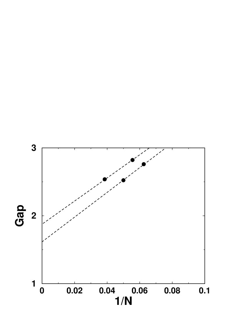
Figure 12: Total energy difference between SRRVB first excited state and GS for the square lattice (16, 18, 20 and 26 site clusters). The Data suggest a non-zero value for the gap in the thermodynamic limit.

In conclusion, SRRVB states on the kagomé lattice allow to capture the specific low energy properties of the model in both trimerized and isotropic limits. In the trimerized model it gives a simple picture of the non magnetic excitations and a selection criterion of the low-energy states which are built by minimizing the number of defaults on strong bond triangles. The number of such states increases like $1.15^{N}$. The states matching this criterion can also be seen as short-range dimer coverings of the triangular lattice formed by strong-bond triangles which confirms, beyond mean field approximation, the relevance of the effective model approach. At the isotropic point, SRRVB states lead to a continuum of non-magnetic excitations in accordance with ED results. Moreover the shape of the SRRVB spectrum is very similar to the exact one and the number of low-lying singlets increases exponentially for all energy range with the size of the system considered.

Finally, these properties of the SRRVB spectrum are not just a property of this kind of states since the SRRVB spectrum has a gap in the case of the square lattice. So one may conjecture that they provide a good description of the low-energy singlet sector of very frustrated magnets only. Work is in progress to test this idea on the pyrochlore lattice.

Acknowledgments: We acknowledge useful discussions with C. Lhuillier, B. Douçot and P. Simon. We are especially grateful to P. Sindzingre for making available unpublished results of exact diagonalization on the kagomé lattice.

5 Appendix: numerical method

Working with SRRVB states as a truncated basis leads to non-trivial numerical difficulties which, as paradoxical as it may seem, make the problem of the determination of the spectrum more tricky in this truncated subspace than in the full space of spin configurations. This is a consequence of the non-orthogonality of RVB states.

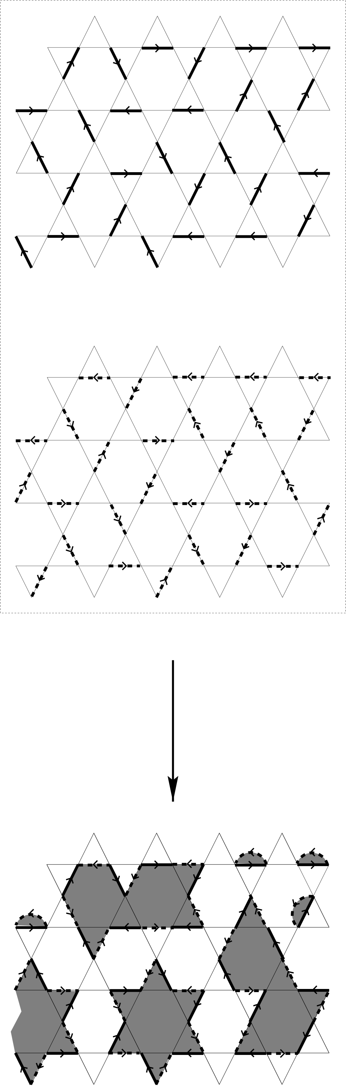
Figure 13: The overlap between two dimer coverings depends on the number of loops in the transition graph (bottom). Note that the relative orientation of dimer coverings in this figure corresponds to the reference orientation which produces a positive overlap.

If $|\varphi_{i}\rangle$ and $|\varphi_{j}\rangle$ are two SRRVB states, the overlap is given by Sutherland

$$\langle\varphi_{i}|\varphi_{j}\rangle=s(\varphi_{i},\varphi_{j})\cdot 2^{n_{b}(\varphi_{i},\varphi_{j})-N/2},$$ (4)

where $n_{b}(\varphi_{i},\varphi_{j})$ is the number of closed loops in the diagram where the two states are superimposed and $s(\varphi_{i},\varphi_{j})=(-1)^{p}$, where $p$ is the number of misoriented dimers compared with the reference orientation (see Fig. 13).

In the case of a non-orthogonal basis, the eigenvalues are solutions of the so-called generalized eigenvalue problem,

$$\det(\langle\varphi_{i}|{\cal H}|\varphi_{j}\rangle-E\langle\varphi_{i}|\varphi_{j}\rangle)=0,$$ (5)

in which the overlap between states appears explicitly. Since we are interested in the structure of the spectrum, we need to diagonalize completely the Hamiltonian and therefore iterative techniques (typically Lanczos) must be avoided. On the other hand, solving (5) with standard routines, one is limited to small systems.

To achieve a complete diagonalization for large systems (typically 36 sites) it is crucial to take into account all the symmetries of the system in order to break the Hilbert space into smaller pieces. This technique is indeed very standard but is usually used in a context where the basis is orthogonal (e.g. spin configurations) which makes it quite convenient. The non-orthogonal case is far less simple and is worth paying some attention.

The aim of this appendix is to explain how it is possible, starting from a set of configurations that can be non-orthogonal, to build an orthonormal basis of vectors that are eigenstates of all the symmetries of the problem in each symmetry sector. Since this linear algebra problem is planned to be solved numerically one is interested in reducing as much as possible the information to be handled. Therefore one does not work explicitly with this orthonormal basis but with linear combinations of suitably chosen configurations called representatives.

The text is organized as follow: we define the representatives, we show how the number of representatives has to be reduced depending on the symmetry sector and finally explain how one can go from representatives to the orthogonal basis of the symmetries eigenvectors.

Representatives. Let us denote by $N_{\cal S}$ the order of the symmetry group of the system and ${{\cal S}_{i}},\;i=1,\dots,N_{\cal S}$ the elements of this group. It is possible to make a partition of the set containing all the configurations in subsets where configurations are related to each other by a symmetry ${\cal S}_{i}$. Each of these $N_{p}$ subset can be represented by a configuration $|p_{i}\rangle,\;i=1,\dots,N_{p}$, called representative, of the subset since by construction all the others can be obtained by applying symmetries on it. From a numerical point of view the set of the representatives is the minimal information needed.

Reduction of the number of representatives in a given symmetry sector. In this section we will consider a given symmetry sector $s$ characterized by a set of characters $\chi_{s}({{\cal S}}_{1})$,…,$\chi_{s}({{\cal S}}_{N_{\cal S}})$. We are going to show that it is not necessary to keep all the representatives to generate a basis in the sector $s$.

Let us consider a given linear configuration of representatives,

$$|\psi\rangle=\sum_{i=1}^{N_{p}}\alpha_{i}\;|p_{i}\rangle.$$ (6)

The true state of $s$ associated to $|\psi\rangle$ is given by remark1 ,

$$|\tilde{\psi}\rangle\triangleq\frac{1}{\sqrt{N_{\cal S}}}\sum_{i=1}^{N_{\cal S}}{{\cal S}_{i}}\;|\psi\rangle=\sum_{i=1}^{N_{p}}\sum_{p=1}^{N_{\cal S}}\alpha_{i}\;\chi_{s}({{\cal S}}_{p})\;|s_{p}(p_{i})\rangle,$$ (7)

where $|s_{p}(p_{i})\rangle$ stands for the image of the configuration $p_{i}$ by the symmetry ${{\cal S}}_{p}$. For a given representative $|p_{i}\rangle$, let us denote by ${\cal E}_{i}$ the set of indices $q$ of the symmetries that leave the configuration $p_{i}$ invariant ($s_{q}(p_{i})=p_{i}$), and $\bar{{\cal E}_{i}}$ the remaining indices. With this notation $|\tilde{\psi}\rangle$ take the form,

$$|\tilde{\psi}\rangle = \sum_{i=1}^{N_{p}}\alpha_{i}\left(\sum_{\begin{subarray}{c}q\in{\cal E}_{i}\end{subarray}}\chi_{s}({{\cal S}}_{q})\right)|p_{i}\rangle$$ (8)

$$+\sum_{i=1}^{N_{p}}\sum_{\begin{subarray}{c}q\in\bar{{\cal E}_{i}}\end{subarray}}\alpha_{i}\;\chi_{s}({{\cal S}}_{q})\;|s_{q}(p_{i})\rangle.$$

Let us denote by ${\cal Q}_{s}$ the list of indices $i$ of the representatives $p_{i}$ such as $\sum_{\begin{subarray}{c}q\in{\cal E}_{i}\end{subarray}}\chi_{s}({{\cal S}}_{q})=0$ in the symmetry sector $s$. It is obvious to note that all the representatives with an index in ${\cal Q}_{s}$ disappear from the first term of eq. (8). What we are going to show is that they also disappear from the second one. Let be $p_{i}$ such as $\sum_{\begin{subarray}{c}q\in{\cal E}_{i}\end{subarray}}\chi_{s}({{\cal S}}_{q})=0$ and $p\in{\cal E}_{i}$. One has $\sum_{\begin{subarray}{c}q\in\bar{{\cal E}_{i}}\end{subarray}}{{\cal S}}_{q}|p_{i}\rangle=\sum_{\begin{subarray}{c}q\in\bar{{\cal E}_{i}}\end{subarray}}\chi_{s}^{*}({{\cal S}}_{p}){{\cal S}}_{p}{{\cal S}}_{q}|p_{i}\rangle=\sum_{\begin{subarray}{c}q\in\bar{{\cal E}_{i}}\end{subarray}}\chi_{s}^{*}({{\cal S}}_{p}){{\cal S}}_{q}|p_{i}\rangle$. This result does not depend on $p\in{\cal E}_{i}$ and thus one does not modify the result by applying $[1/{\text{Card}}({{\cal E}_{i}})]\sum_{\begin{subarray}{c}p\in{\cal E}_{i}\end{subarray}}$ on the previous expression which proves what was announced. This leads to a reduction of the number of representatives in the symmetry sector $s$, namely $N_{s}=N_{p}-{\text{Card}}({\cal Q}_{s})$.

From non-orthogonal representatives to the orthonormal basis of symmetries eigenvectors. In the general case of non-orthogonal representatives, it is convenient to introduce a mixing matrix $\mu^{s}$ in order to build the orthonormal basis of symmetries eigenvectors. We will considerer from now linear combinations of mixed representatives,

$$|l\rangle=\sum_{j=1}^{N_{s}}\mu^{s}_{lj}|p_{j}\rangle.$$ (9)

All the problem is to chose $\mu^{s}$ such as the symmetrized states $|\tilde{l}\rangle$ of $|l\rangle$ according to (7) form an orthonormal basis: $\langle\tilde{l}|\tilde{m}\rangle=\delta_{lm}$. Let us show how this condition writes in the cases of orthogonal and non-orthogonal representatives.

Orthogonal case. In this simple case where $\langle p_{i}|p_{j}\rangle=\delta_{ij}$, the condition $\langle\tilde{l}|\tilde{m}\rangle=\delta_{lm}$ is,

$$\delta_{lm} =\sum_{i,j=1}^{N_{s}}\sum_{q=1}^{N_{\cal S}}{\mu^{s*}_{jl}}\mu^{s}_{mi}\langle p_{j}|{{\cal S}}_{q}|p_{i}\rangle$$

$$=\sum_{i,j=1}^{N_{s}}\mu^{s*}_{jl}\mu^{s}_{mi}\left(\sum_{q\in{\cal E}_{i}}\chi_{s}({{\cal S}}_{q})\right)\delta_{ij}$$

$$=\sum_{i,j=1}^{N_{s}}\mu^{s*}_{jl}\mu^{s}_{mi}{\text{deg}}(p_{i})\delta_{ij},$$ (10)

where $\chi_{s}({{\cal S}}_{p})$ is the character of the symmetry ${{\cal S}}_{p}$ in the sector $s$, ${\text{deg}}(p_{i})$ the degeneracy of representative $p_{i}$ (i.e. the number of symmetries under which it is invariant remark2 ), $s_{p}(p_{i})$ the image of the configuration $p_{i}$ by ${{\cal S}}_{p}$, and $N_{s}$ the size of the sector $s$.

It is easy to see that

$$\mu^{s}_{ij}=\delta_{ij}/\sqrt{{\text{deg}}(p_{i})}$$ (11)

fulfills (10)

General case. In the non-orthogonal case, the condition (10) now reads,

$$\delta_{lm}=\sum_{i,j=1}^{N_{s}}\mu^{s*}_{jl}\mu^{s}_{mi}\tilde{I}_{ij}$$ (12)

where,

$$\tilde{I}_{ij}=\sum_{p=1}^{N_{\cal S}}\chi_{s}({{\cal S}}_{p})\langle p_{j}|s_{p}(p_{i})\rangle$$ (13)

Here again, the indices $i$ and $j$ runs from $1$ to $N_{s}$ (the size of the sector $s$). To determine $\mu^{s}$ we diagonalize $\tilde{I}$ :

$$P^{\dagger}\tilde{I}P={\text{Diag}}(d_{1},\dots,d_{N_{s}})$$ (14)

One can check that,

$$\mu^{s}_{ij}=\frac{1}{\sqrt{d_{i}}}\;P_{ij}$$ (15)

satisfies condition (12).

The basis $\{|\tilde{l}\rangle\}$ is orthogonal and in this new basis the Hamiltonian is block diagonal, each block corresponding to one symmetry sector. Thus, it only remains to diagonalize the Hamiltonian in each of these representations to get the whole spectrum :

$$\langle\tilde{l}|{\cal H}|\tilde{m}\rangle=\sum_{i,j=1}^{N_{s}}\sum_{p=1}^{N_{\cal S}}\mu^{s*}_{jl}\mu^{s}_{mi}\chi_{s}({{\cal S}}_{p})\langle p_{j}|{\cal H}|s_{p}(p_{i})\rangle$$ (16)

In conclusion the procedure described above turns the generalized eigenvalue problem of $n\times n$ matrices into $2\times N_{s}$ conventional diagonalizations of $\sim(n/N_{s})\times(n/N_{s})$ matrices. The point we now want to stress is that the treatment described above is exact and does not introduce approximation. The subspace of RVB states is a truncated subspace in the sense that it is not stable with respect to an application of the Hamiltonian and only the RVB restricted Hamiltonian is studied. But, the use of symmetries does not act as a new restriction of the Hamiltonian in each representation of the symmetry group. In the new basis the Hamiltonian and the overlap matrix are actually block diagonal, each block corresponding to one representation. Thus the spectrum obtained as well as mean values of operators calculated are the same as those one would obtain by solving with brute-force the generalized eigenvalue problem if it was possible.

References

- (1) C.K. Majumdar and D. Ghosh, J. Math. Phys. 10, (1969), 1388.
- (2) C. Waldtmann, H.-U. Everts, B. Bernu, C. Lhuillier, P. Sindzingre, P. Lecheminant, L. Pierre, European Physical Journal B 2, (1998), 501.
- (3) B. Canals, private communication.
- (4) M. Mambrini, J. Trébosc and F. Mila, Phys. Rev. B 59,(1999), 13806.
- (5) C. Zeng and V. Elser, Phys. Rev. B 42, (1990), 8436.
- (6) R. Singh and D. Huse, Phys. Rev. Lett. 68, (1992), 1766.
- (7) P. Leung and V. Elser, Phys. Rev. B 47, (1993), 5459.
- (8) C. Zeng and V. Elser, Phys. Rev. B 51, (1995), 8318.
- (9) P. Sindzingre, P. Lecheminant and C. Lhuillier, Phys. Rev. B 50, (1994), 3108.
- (10) T. Nakamura and S. Miyashita, Phys. Rev. B 52, (1995), 9174.
- (11) P. Lecheminant, B. Bernu, C. Lhuillier, L. Pierre and P. Sindzingre, Phys. Rev. B 56, (1997), 2521.
- (12) P. Fazekas and P.W. Anderson, Philos. Mag. 30, (1974), 423.
- (13) P.W. Anderson, Science 235, (1987), 1196.
- (14) V. Elser, Phys. Rev. Lett. 62, (1989), 2405.
- (15) M. Fisher, Phys. Rev. 124, (1961), 1664.
- (16) P. Kasteleyn, Physica 27, (1961), 1209; P. Kasteleyn, J. Math. Phys. 4, (1963), 287.
- (17) F. Mila, Phys. Rev. Lett. 81, (1998), 2356.
- (18) In Ref Mila , the model of Fig. 1 was called “dimerized kagomé”. This terminology is misleading since the local units consist of three sites. So we will use the more natural terminology of “trimerized kagomé model” throughout.
- (19) B. Sutherland, Phys. Rev. B 37, 3786 (1988).
- (20) Note that the definition of implies trivially that it is an eigenstate of each with the eigenvalue .
- (21) It is not immediately clear that what we call does not depend on the sector since it involves sums over characters of this given sector. The argument is the following: where is arbitrarily chosen in . This last point is due to the fact that is a subgroup of . After a summation on over using the property one gets . Only two possibility can occur: either which is the case of eliminated representatives, or , which indeed does not depend on the sector .