Vortex-glass phases in type-II superconductors

Abstract

A review is given on the theory of vortex-glass phases in impure type-II superconductors in an external field. We begin with a brief discussion of the effects of thermal fluctuations on the spontaneously broken $U(1)$ and translation symmetries, on the global phase diagram and on the critical behaviour. Introducing disorder we restrict ourselves to the experimentally most relevant case of weak uncorrelated randomness which is known to destroy the long-ranged translational order of the Abrikosov lattice in three dimensions. Elucidating possible residual glassy ordered phases, we distinguish between positional and phase-coherent vortex glasses. The study of the behaviour of isolated vortex lines and their generalization – directed elastic manifolds – in a random potential introduces further important concepts for the characterization of glasses. The discussion of elastic vortex glasses, i.e., topologically ordered dislocation-free positional glasses in two and three dimensions occupy the main part of our review. In particular, in three dimensions there exists an elastic vortex-glass phase which still shows quasi-long-range translational order: the ‘Bragg glass’. It is shown that this phase is stable with respect to the formation of dislocations for intermediate fields. Preliminary results suggest that the Bragg-glass phase may not show phase-coherent vortex-glass order. The latter is expected to occur in systems with weak disorder only in higher dimensions (or for strong disorder, as the example of unscreened gauge glasses shows). We further demonstrate that the linear resistivity vanishes in the vortex-glass phase. The vortex-glass transition is studied in detail for a superconducting film in a parallel field. Finally, we review some recent developments concerning driven vortex-line lattices moving in a random environment.

1 Introduction

Since its discovery by Kammerlingh Onnes in 1911, superconductivity has attracted generations of physicists. In 1935 Fritz and Heinz London (see e.g. [London 1950] (?)) developed a very successful phenomenological theory which describes both the perfect conductivity as well as the perfect diamagnetism of superconductors. As discussed later by [London 1950] (?) this theory can be motivated by considering superconductivity as a phenomenon characterized by long-range order of momentum ${\bf p}$. Bohr-Sommerfeld quantization $\oint{\bf p}_{s}d{\bf s}=nh$ on a torus gives fluxoid quantization [London 1950]. [Ginzburg and Landau 1950] (?) combined London’s electrodynamics of a superconductor with Landau’s theory of phase transitions, creating a powerful phenomenological description of superconductivity. The transition to the superconducting phase corresponds here to the breaking of the U(1) symmetry of the complex order parameter $\Psi$ and the appearance of off-diagonal long-range order (ODLRO).

In a pioneering work [Abrikosov 1957] (?) showed the existence of a second type of superconductors which (for sufficiently strong external magnetic field) allows for a penetration of quantized magnetic flux in the form of vortex lines, which form a triangular lattice, reducing the perfect diamagnetism and creating a source for dissipation due to the motion of the vortex-line core driven by the transport current. In this case the continuous translational symmetry of the system is broken in addition to the $U(1)$ symmetry. Effects from thermal fluctuations, although studied already since 1960, were considered to be extremely small because of the large correlation length and low transition temperatures of conventional superconductors [Ginzburg 1961].

To keep the superconducting properties, vortices have to be prevented from moving by pinning centers. An early theory of pinning of isolated vortex lines [Anderson and Kim 1964] shows the absence of dissipation only at zero temperature. Thermally activated hopping leads to a small but finite dissipation at low temperatures (as compared to the height of energy barriers). [Larkin 1970] (?) extended this theory to the Abrikosov vortex-line lattice, showing the destruction of its translational long-range order. Although – in principle – the Abrikosov phase could thence be considered not to really differ from a pinned vortex-line liquid (and hence from the normal phase), the generic phase diagram of conventional superconductors was assumed to practically be that of [Abrikosov 1957] (?) with a now finite correlation length of the vortex-line array.

In the 1980s this picture was changed by two initially unrelated developments: the discovery of high-$T_{c}$ superconductors by [Bednorz and Müller 1986] (?) and the much better understanding of random system, in particular of spin glasses and of random-field systems (for a recent review see [Young 1998] (?)). In the high-$T_{c}$ superconductors with their elevated transition temperatures and pronounced anisotropy, fluctuation effects became now very important as can be seen for instance from the observed melting of the vortex-line lattice [Cubitt et al. 1993, Zeldov et al. 1995]. Moreover, for pure systems it was demonstrated [Moore 1989, Moore 1992, Ikeda et al. 1992] that thermal fluctuations – which prohibit true long-range translational order of the vortex-line lattice (VLL) only in $d\leq 2$ dimensions – destroy the ODLRO of the gauge invariant order parameter in the Abrikosov phase even in higher dimensions. Thus, in three dimensions thermal fluctuations restore the $U(1)$ symmetry of the Ginzburg-Landau Hamiltonian but nevertheless allow for the existence of a vortex lattice. This finding is paralleled by an earlier observation of [Schafroth 1955] (?) that an external magnetic field above a critical strength destroys Bose-Einstein condensation of an ideal Bose gas which still shows some remanent diamagnetic moment.

For systems with disorder the idea emerged that despite of the destruction of true translational long-range order the system could show a phase with some kind of glassy long-range order, the “vortex glass” [Fisher 1989]. Because of the residual rigidity in the vortex-line array, arbitrarily large energy barriers now exist, leading to a highly non-linear resistivity [Feigel’man and Vinokur 1990, Fisher 1989, Feigel’man et al. 1989, Nattermann 1990, Fisher et al. 1991a]

$$\rho(j)\sim e^{-(j_{\rm t}/j)^{\mu}}$$ (1.1)

where $\mu$ denotes an exponent $0\leq\mu\leq 1$ and $j_{\rm t}$ a threshold current. Since the linear resistivity vanishes, the system is truly superconducting.

In the following years vortex pinning and depinning as well as flux creep under the action of an external current was investigated by many researchers to a great extent. A brilliant summary of the results of these efforts till 1994 is given in the extensive review article by [Blatter et al. 1994] (?) (see also [Brandt 1995] (?), [Gammel et al. 1998] (?), [Giamarchi and Le Doussal 1998] (?)). It is not the intention of the present article to provide an updated version of these reviews by discussing the results obtained since then. Instead, we want to focus here mainly on one particular aspect of the theory, namely on the discussion of the equilibrium phase diagram of weakly disordered type-II superconductors in an external magnetic field. We want to demonstrate that the notion of a ‘vortex glass’ is not a blurred expression for the hopelessly intricate situation in a disordered system (as some physicists may still claim), but that it has a well defined meaning. The knowledge of the equilibrium properties is also important for the proper understanding of situations close to equilibrium, e.g. for the discussion of flux creep under the influence of a small external current.

Despite of the conclusion common to all authors mentioned above of expecting a non-analytic current-density dependence of the resistivity in the glassy phase it seems to be indicated to refer here also to the differences between these approaches. [Fisher 1989] (?) and [Fisher et al. 1991a] (?) in their definition of the glassy phase started from correlation functions measuring ODLRO and focused on the long-range (glassy) order of phases (see chapter 2.4). On the other hand, [Feigel’man et al. 1989] (?), [Nattermann 1990] (?) and subsequently [Korshunov 1993] (?) and [Giamarchi and Le Doussal 1994] (?) considered primarily the glassy order of the vortex-line array, i.e., they focused on the positions of the vortex lines. In both cases, the expression ‘vortex glass’ was used. The above mentioned differences in the lower critical dimensions for the breaking of the $U(1)$ and of the translational symmetry in pure systems however suggests, that there may be also different lower critical dimensions for a phase-coherent and a positional vortex glass. In this review we concentrate mainly on the positional glass. If, in particular, the positional vortex glass is free of large dislocation loops such that an elastic description of the vortex array is possible, the positional vortex glass will be called elastic vortex glass. The most prominent example of an elastic vortex glass is its three-dimensional version: the so-called ‘Bragg-glass’ (for a recent brief review see [Giamarchi and Le Doussal 1998] (?)). Whether non-elastic vortex-glass phases exist is still unclear.

Systems with columnar disorder which leads to the formation of the so-called ‘Bose-glass’ phases (see e.g. [Täuber and Nelson 1997] (?)) will be completely neglected in this review since their physics is substantially different from that for systems with point disorder, to which we restrict ourselves here. However, we also include the discussion of various phases found for driven systems far from equilibrium, which share some features with the equilibrium phase diagram.

The article is organized as follows. In chapter 2 we present a brief summary of the Ginzburg-Landau theory of type-II superconductors and a short discussion of the influence of thermal fluctuations and of the effect of point disorder in the critical region. We also define the different types of vortex-glass order and give a brief account of results obtained for models with strong disorder – the so-called gauge glasses. In chapter 3 we review the behaviour of a single vortex line and its generalizations – $D$-dimensional directed manifolds – in a random potential. This simple, but not at all trivial system allows for a discussion of different aspects of glassiness of a system. Chapter 4 is devoted to the superconducting film in a parallel field, a geometry which allows for a very detailed description of the vortex glass phase as well as of the transition to the normal phase both for the static and dynamic quantities. In chapter 5 we discuss an impure superconducting film in a field perpendicular to the film plane. It turns out that dislocations destroy the positional vortex-glass phase in this geometry. The ‘Bragg-glass’ phase of a bulk superconductor as well as its stability with respect to dislocations is considered in chapter 6. A short account of recent activities on driven vortex lattices in impure superconductors is presented in chapter 7. We close the paper with a brief summary of the results of this article (chapter 8). The appendix contains some technicalities and a list of recurrent symbols.

2 Ginzburg-Landau description

In this chapter we give a very brief introduction into the mean-field theory and the effects arising from thermal and disorder fluctuations in type-II superconductors in the framework of the Ginzburg-Landau theory. Since there is extensive (and partially contradicting) literature on thermal effects it is impossible to include all related references. However, we attempt to include the most recent articles on the subject which may serve as more comprehensive guides to further references.

2.1 The Ginzburg-Landau model

In 1950 Ginzburg and Landau proposed a phenomenological description of superconductors by introducing a two-component order parameter $\Psi({\bf r})=|\Psi({\bf r})|e^{i\phi({\bf r})}$ which couples in a gauge-invariant form to the magnetic field described by the vector potential ${\bf A}({\bf r})$ [Ginzburg and Landau 1950]. The density $n_{\rm s}({\bf r})$ of superconducting charge carriers (i.e., of the Cooper pairs), which is a central quantity of the earlier London theory [London and London 1935], is related to $\Psi({\bf r})$ by $n_{\rm s}({\bf r})=|\Psi({\bf r})|^{2}$. The Ginzburg-Landau (GL) free energy is given by

$${\cal H}_{\rm GL} = \frac{1}{2}\int d^{d}r\ \Big{\{}\beta\Big{(}|\Psi|^{2}+\frac{\alpha}{\beta}\Big{)}^{2}$$ (2.1)

$$+\frac{\hbar^{2}}{m}\Big{|}\Big{(}i{\mbox{\boldmath${{\nabla}}$}}-\frac{2\pi}{\Phi_{0}}{\bf A}\Big{)}\Psi\Big{|}^{2}+\frac{1}{4\pi}({\mbox{\boldmath${{\nabla}}$}}\wedge{\bf A}-{\bf H})^{2}\Big{\}},$$

where $\Phi_{0}=hc/2e$ denotes the flux quantum, $\alpha(T)\propto(T-T_{\rm c0})$, $T_{\rm c0}$ is the mean-field transition temperature, ${\bf H}$ is the external field, and $m$ denotes the mass of a Cooper pair. The GL free energy is characterized by two basic length scales, the coherence length $\xi$ and the penetration depth $\lambda$, which are related to the parameters of ${\cal H}_{\rm GL}$ by

$$\xi^{2}(T) = \frac{\hbar^{2}}{2m|\alpha(T)|},$$ (2.2a)

$$\lambda^{2}(T) = \frac{mc^{2}}{4\pi|\Psi_{0}|^{2}(2e)^{2}}.$$ (2.2b)

Here $|\Psi_{0}|^{2}=|\alpha|/\beta$ denotes the saturation value of $|\Psi|^{2}$ in a homogeneous current free state for $T<T_{\rm c0}$ and ${\bf H}={\bf 0}$. For our further discussion it is convenient to use the following rescaling to introduce dimensionless quantities $\Psi^{\prime}$, ${\bf A}^{\prime}$ and ${\bf r}^{\prime}$

$$\Psi = \Psi^{\prime}|\alpha/\beta|^{1/2},\quad{\bf A}=\frac{\Phi_{0}}{2\pi\xi}{\bf A}^{\prime},\quad{\bf r}={\bf r}^{\prime}\xi.$$ (2.3)

This leads to

$$\frac{1}{T}{\cal H}_{\rm GL} = \frac{1}{4\pi}\left(\frac{|\tau_{\rm c0}|^{4-d}}{2{\rm Gi}}\right)^{1/2}\int d^{d}r^{\prime}\Big{\{}\frac{1}{2}(|\Psi^{\prime}|^{2}+\alpha/|\alpha|)^{2}$$ (2.4)

$$+|(i{\mbox{\boldmath${{\nabla}}$}}^{\prime}-{\bf A}^{\prime})\Psi^{\prime}|^{2}+\kappa^{2}\Big{(}{\mbox{\boldmath${{\nabla}}$}}^{\prime}\wedge{\bf A}^{\prime}-{\bf H}/{H_{\rm c2}^{\rm MF}}\Big{)}^{2}\Big{\}}.$$

Here we introduced the Ginzburg number

$${\rm Gi}\equiv\left(\frac{T}{4\pi\xi^{d}(0)\beta|\Psi_{0}(0)|^{4}}\right)^{2}=\left(\frac{T}{\xi^{d}(0)H_{\rm c}^{2}(0)}\right)^{2},$$ (2.5)

the Ginzburg-Landau parameter $\kappa\equiv\lambda/\xi$ and the reduced temperature $\tau_{\rm c0}\equiv(T_{\rm c0}-T)/T_{\rm c0}$. $H_{\rm c2}^{\rm MF}\equiv\Phi_{0}/2\pi\xi^{2}$ is the mean-field upper critical field and $H_{\rm c}^{2}=4\pi\beta|\Psi_{0}|^{4}$ is the thermodynamic critical field.

2.2 Mean-field theory

Within mean-field (MF) theory, the GL free energy has to be minimized with respect to the fields $\Psi({\bf r})$ and ${\bf A}({\bf r})$. The resulting GL-equations

$$(i{\mbox{\boldmath${{\nabla}}$}}^{\prime}-{\bf A}^{\prime})^{2}\Psi^{\prime}+\frac{\alpha}{|\alpha|}\Psi^{\prime}+|\Psi^{\prime}|^{2}\Psi^{\prime}=0$$ (2.6)

and (for $\alpha<0$)

$$\kappa^{2}\frac{1}{|\Psi^{\prime}|^{2}}{\mbox{\boldmath${{\nabla}}$}}\wedge({\mbox{\boldmath${{\nabla}}$}}\wedge{\bf A}^{\prime})+{\bf A}^{\prime}=-{\mbox{\boldmath${{\nabla}}$}}^{\prime}\phi$$ (2.7)

then have to be solved with the appropriate boundary conditions. As is clear from equation (2.4), the only two parameters which will enter the solution in the bulk, are the GL-parameter $\kappa$, which plays the role of an inverse effective charge of the $\Psi$ field, and the strength of the external magnetic field ${\bf H}^{\prime}={\bf H}/H_{\rm c2}^{\rm MF}$.

For $\kappa<1/\sqrt{2}$ (type-I superconductors), mean-field theory yields for $T<T_{\rm c0}$ and $H<H_{\rm c}(T)$ a phase with vanishing resistance and perfect diamagnetism. The transition to the normal phase at $H_{\rm c}(T)$ is first order.

For $\kappa>1/\sqrt{2}$ (type-II superconductors), on the other hand, perfect diamagnetism exists only up to the field $H_{\rm c1}^{\rm MF}\approx(H_{\rm c2}^{\rm MF}/{2\kappa^{2}})(\ln\kappa+0.08)$. For larger fields, magnetic flux penetrates the sample in the form of quantized vortex lines, each carrying a flux quantum $\Phi_{0}$. The energy per unit length of the vortex line is therefore given by $\varepsilon_{\rm l}=(\Phi_{0}/4\pi)H_{\rm c1}\simeq\varepsilon_{0}\ln\kappa$ with $\varepsilon_{0}=(\Phi_{0}/4\pi\lambda)^{2}$ as the important energy scale per unit length.

The vortex lines form a triangular ‘Abrikosov’ lattice [Abrikosov 1957, Kleiner et al. 1964] of spacing $a_{\triangle}=(2/\sqrt{3})^{1/2}a$, where $a\equiv(\Phi_{0}/B)^{1/2}$. The Abrikosov lattice (or ‘mixed’) phase shows both broken translational symmetry and off-diagonal long-range order (ODLRO), i.e., broken U(1) symmetry of the order parameter. Both broken symmetries vanish simultaneously if $H$ reaches $H_{\rm c2}^{\rm MF}$. One should however take into account that the correlation function for ODLRO (see chapter 2.3.2) $\langle\Psi^{\ast}({\bf r})\,\Psi({\bf r}^{\prime})\rangle$ – even if calculated in MF approximation – shows strong spatial variations due to the rapid change of the phase. Indeed, for a system of radius $R$ the tangential phase gradient on the boundary is of the order $R/2a^{2}$ which corresponds to a phase change of $2\pi$ on a distance $l_{\phi}\approx 4\pi a^{2}/R$ (with $a\approx 100{\rm nm}$ and $R\approx 1{\rm cm}$, $l_{\phi}\approx 10^{-2}{\rm nm}$ which is smaller than an atom, see [Brandt 1974] (?)). Thus $\langle\Psi^{\ast}({\bf r})\,\Psi({\bf r}^{\prime})\rangle$ cannot be very meaningful as a physical observable. Quantities with a physical significance should be in particular gauge invariant. In the GL-description these are the amplitude $|\Psi|$ of the order parameter, the ‘super-velocity’ ${\mbox{\boldmath${{\nabla}}$}}\phi-\frac{2\pi}{\Phi_{0}}{\bf A}\equiv{\mbox{\boldmath${{\nabla}}$}}\tilde{\phi}$ and the magnetic induction ${\bf B}={\mbox{\boldmath${{\nabla}}$}}\wedge{\bf A}$. All other physical quantities can be expressed in these fields, e.g. the current density can be written as

$${\bf j}=-\frac{2e\hbar}{m}|\Psi|^{2}{\mbox{\boldmath${{\nabla}}$}}\tilde{\phi}\,.$$ (2.8)

In treating the vortex system, two main approximations have been used: the lowest Landau level (LLL) approximation, which is valid sufficiently close to $H_{\rm c2}^{\rm MF}$ ($H\gtrsim\frac{1}{3}H_{\rm c2}^{\rm MF}$), and the London approximation, which is valid at intermediate and small fields $B\lesssim 0.2H_{\rm c2}^{\rm MF}$, where $\xi\ll a$. The precise range of applicability of the LLL is still under debate (see e.g. [O’Neill and Moore 1993] (?), [Li and Rosenstein 1999] (?) and references therein).

In the London approximation one neglects amplitude inhomogeneities, $|\Psi|=|\Psi_{0}|$, which leads to a diverging energy density at the vortex cores. The position ${\bf r}_{i}(s)$ of these cores is parameterized by the label $i$ of a vortex and the variable $s$ along the contour of the vortex lines. The Ginzburg-Landau Hamiltonian takes then the form

$${{\cal H}}_{\rm London}=\frac{1}{2}\int d^{d}r\left\{\frac{\hbar^{2}}{m}|\Psi_{0}|^{2}({\mbox{\boldmath${{\nabla}}$}}\phi+\frac{2\pi}{\Phi_{0}}{\bf A})^{2}+\frac{1}{4\pi}({\mbox{\boldmath${{\nabla}}$}}\wedge{\bf A}-{\bf H})^{2}\right\}\,.$$ (2.9)

This functional has to be regularized near the vortex cores, e.g. by excluding tubes of radius $\xi$ around the vortex cores from the volume integration. The phase $\phi({\bf r})$ of the complex order parameter is a multivalued function since $\phi$ changes by $2\pi$ along a path surrounding a vortex line. We decompose $\phi$ now into a vortex part $\phi_{\rm v}$ and a “spin-wave” part $\phi_{\rm sw}$. The vortex part is assumed to fulfill the saddle point equation apart from the position of the vortices ${\bf r}_{i}(s)$. With the London gauge ${\mbox{\boldmath${{\nabla}}$}}\cdot{\bf A}=0$ this yields

$${\mbox{\boldmath${{\nabla}}$}}^{2}\phi_{\rm v}({\bf r})=0\,,\quad{\bf r}\not={\bf r}_{i}(s)$$ (2.10)

and

$${\mbox{\boldmath${{\nabla}}$}}\wedge({\mbox{\boldmath${{\nabla}}$}}\phi_{\rm v})=2\pi{\bf m}({\bf r})\,.$$ (2.11)

Here ${\bf m}({\bf r})$ denotes the vortex-density field

$${\bf m}({\bf r})=\sum\limits_{i}m_{i}\int ds\frac{d{\bf r}_{i}(s)}{ds}\delta^{(3)}({\bf r}_{i}(s)-{\bf r})\,,$$ (2.12)

where the integration is along the vortex line $i$ which carries the vorticity $m_{i}=\pm 1$. If the spin-wave part $\phi_{\rm sw}({\bf r})$ vanishes on the surface of the sample, $\phi_{\rm sw}$ and $\phi_{\rm v}$ decouple. Since the vector potential ${\bf A}$ appears only quadratically in $H_{\rm GL}$ it can be integrated out by using the saddle-point equation which is the second GL-equation in the phase-only approximation

$${\bf A}+\lambda^{2}{\mbox{\boldmath${{\nabla}}$}}\wedge({\mbox{\boldmath${{\nabla}}$}}\wedge{\bf A})=-\frac{\Phi_{0}}{2\pi}{\mbox{\boldmath${{\nabla}}$}}\phi_{\rm v}.$$ (2.13)

Taking the curl of (2.13) gives the modified London equation

$$\lambda^{2}{\mbox{\boldmath${{\nabla}}$}}^{2}{\bf B}({\bf r})-{\bf B}({\bf r})=\Phi_{0}{\bf m}({\bf r}),$$ (2.14)

where ${\bf B}={\mbox{\boldmath${{\nabla}}$}}\wedge{\bf A}$ can now completely be expressed in terms of the vortex degrees of freedom given by the vortex density field ${\bf m}({\bf r})$, equation (2.12). The London Hamiltonian then takes the form

$${\cal H}_{\rm London}=\frac{1}{2}\int d^{d}r\left\{\frac{\hbar^{2}}{m}|\Psi_{0}|^{2}({\mbox{\boldmath${{\nabla}}$}}\phi_{\rm sw})^{2}+\frac{\lambda^{2}}{4\pi}({\mbox{\boldmath${{\nabla}}$}}\wedge{\bf B})^{2}+\frac{1}{4\pi}({\bf B}-{\bf H})^{2}\right\}\,.$$ (2.15)

In most parts of this review we will use the London picture, since it remains valid in the vortex phases we will describe, in particular in the elastic glass phases.

The elasticity theory of the Abrikosov lattice for an isotropic superconductor was worked out by Brandt (?, ?). The distortion of a vortex line is described by a two-component displacement field ${\bf u}({\bf X},z)$, where the lattice vector ${\bf X}\equiv{\bf X}_{n,m}=((2n+m)a_{\triangle}/2,m\sqrt{3}a_{\triangle}/2)$ denotes the rest position of the vortex line in the plane perpendicular to ${\bf H}=H\hat{{\bf z}}$. In many cases one can go over to the continuum description: ${\bf u}({\bf X},z)\to{\bf u}({\bf x},z)\equiv{\bf u}({\bf r})$. On large scales $L\gg\lambda$ the elastic energy of the vortex-line lattice is then given by

$${\cal H}_{\rm el}=\frac{1}{2}\int d^{2}xd^{d-2}z\left\{c_{11}({\mbox{\boldmath${{\nabla}}$}}_{\perp}\cdot{\bf u})^{2}+c_{66}({\mbox{\boldmath${{\nabla}}$}}_{\perp}\wedge{\bf u})^{2}+c_{44}({\mbox{\boldmath${{\nabla}}$}}_{\parallel}{\bf u})^{2}\right\},$$ (2.16)

where $c_{11}\approx c_{44}\approx{\bf B}^{2}/4\pi$. The Abrikosov phase is characterized in particular by a non-zero shear modulus $c_{66}\approx\frac{B\Phi_{0}}{(4\pi\lambda)^{2}}\left(1-\frac{B}{H_{\rm c2}^{\rm MF}}\right)^{2}$, which vanishes both at $H_{\rm c2}$ and $H_{\rm c1}$, reaching a maximum of $c_{66}\approx H_{\rm c1}H_{\rm c2}/56\pi$ in between. One should however take into account that the elastic free energy is in general non-local, which is expressed in a strong dispersion of $c_{11}$ and $c_{44}$ on scales smaller than $\lambda$ (see, e.g., [Brandt 1991] (?)).

In the absence of pinning centres, the system in the Abrikosov phase behaves superconducting only for currents parallel to the magnetic field. For currents with components perpendicular to the field the Lorentz force drives the vortex-line array, which leads to metallic behaviour with resistivity $\rho\approx\rho_{\rm n}B/H_{\rm c2}$ [Bardeen and Stephen 1965]. Here $\rho_{\rm n}$ is the resistivity of the normal phase.

Before we come to the discussion of fluctuation effects, we want to consider a possible extension of the model (2.1) which describes an isotropic superconductor. High-$T_{\rm c}$ superconductors, however, are characterized by a pronounced layer structure, which results in an inhomogeneity and in a strong spatial anisotropy of the effective mass of the Cooper pair such that $m$ is replaced by $M=m/\epsilon^{2}$ for electrons moving perpendicular to the layers. Typical values for $\epsilon$ are $\epsilon_{\rm YBCO}\approx 0.16$ and $\epsilon_{\rm BSCCO}\approx 10^{-2}$ for the two high-$T_{\rm c}$ materials YBCO and BSCCO. It was shown by [Blatter et al. 1992] (?) (for a more detailed discussion, see [Blatter et al. 1994] (?)), that in the case of $\kappa\gg 1$ the result for a thermodynamic quantity ${\cal Q}(\vartheta,H,T,\xi,\lambda,\epsilon,\Delta)$ of an anisotropic superconductor (where $\vartheta$ denotes the angle between the magnetic field direction and the $xy$ plane, and $\Delta$ the strength of disorder) can be obtained from the corresponding result $\widetilde{\cal Q}$ for the isotropic system by the relation

$${\cal Q}(\vartheta,H,T,\xi,\lambda,\epsilon,\Delta)=s_{\cal Q}\ \widetilde{\cal Q}(\epsilon_{\vartheta}H,T/\epsilon,\xi,\lambda,\Delta/\epsilon),$$ (2.17)

where $\epsilon_{\vartheta}^{2}=\epsilon^{2}\cos^{2}\vartheta+\sin^{2}\vartheta$, $s_{V}=s_{E}=s_{T}=\epsilon$ for volume, energy and temperature, and $s_{B}=s_{H}=1/\epsilon_{\vartheta}$ for magnetic fields. Since $T$ and $\Delta$ are increased by a factor $1/\epsilon$ with respect to the isotropic system, it is clear that fluctuation effects, which will be considered in the following sections, are drastically enlarged (by a factor up to 100) in these materials.

If the spatial anisotropy is so large that the coherence length $\xi_{z}=\xi\epsilon$ in $z$ direction becomes of the order of the layer spacing $s$, the discreteness of the layer structure becomes relevant. In this case, new effects such as a decoupling of the layers [for $B>B_{\rm 2D}\approx(\epsilon/s)^{2}\ln(s/\xi)$] may occur. The appropriate description is then the Lawrence-Doniach model [Lawrence and Doniach 1971]. We will not attempt to cover in this review also these particular features of strongly layered materials, instead we restrict ourselves in the following to the discussion of the isotropic superconductor, knowing that the results for the anisotropic case can be found from the relation (2.17).

The neglect of layer-effects is also supported by the following argument: Our theoretical analysis will be mainly based on the elastic description of the vortex lattice and our main interest concerns features on large length scales. Sufficiently weak disorder will indeed effectively couple to the vortex lattice only on very large length scales, where the elasticity of the lattice may be described by local elasticity theory. Since within the London approach all information about anisotropy and even about the layered structure is encoded in the dispersion of the elastic constants, we expect that the large-scale properties are independent of these details (provided that one is in the parameter regime where the London approach is valid and that disorder is sufficiently weak).

2.3 Thermal fluctuations

So far we have ignored the influence of fluctuations, i.e., of configurations which do not fulfill the GL equations. These can be taken into account if we interpret the GL free energy as an effective Hamiltonian from which the true free energy ${\cal F}(T,{\bf H})$ has to be calculated as

$${\cal F}(T,{\bf H})=-T\ln\left(\int{\cal D}\Psi{\cal D}{\bf A}e^{-{\cal H}_{\rm GL}/T}\right).$$ (2.18)

Since the only material independent common feature of type-II superconductors is flux quantization it is natural to build from $\Phi_{0}$ and $T$ a characteristic length scale [Fisher et al. 1991a]

$$\Lambda_{T}\equiv\frac{\Phi_{0}^{2}}{16\pi^{2}T}\approx 2\cdot 10^{8}\frac{\textrm{\AA}}{T[{\textrm{K}}]},$$ (2.19)

which is the same for all materials. Since the energy per unit length of a vortex line (and hence also its stiffness constant $\varepsilon_{\parallel}$, see below) is of the order $\varepsilon_{0}=(\Phi_{0}/4\pi\lambda)^{2}$, $\Lambda_{T}$ denotes the length scale on which the mean squared displacement of a vortex line is of order $\lambda$. Since $\Lambda_{T}$ is so large, thermal fluctuation effects are expected to be small (however, see our remark about strongly anisotropic systems in the previous chapter 2.2). In $d=3$ dimensions the Ginzburg number can be expressed as ${\rm Gi}\approx(\kappa\lambda(0)/\Lambda_{T})^{2}$. As can be seen directly from (2.4) and (2.18) the contribution from fluctuations in $\Psi({\bf r})$ and ${\bf A}({\bf r})$ will indeed be small, if both ${\rm Gi}\ll|\tau_{\rm c0}|^{4-d}$ and $\kappa\gg 1$.

2.3.1 Zero external field

In zero external field, ${\bf H}={\bf 0}$, to begin with, it was shown by [Halperin et al. 1974] (?) that for type-I superconductors, where $\kappa<1/\sqrt{2}$ and typically ${\rm Gi}\ll 1$ (e.g., ${\rm Gi}\approx 10^{-13}$ for aluminium), fluctuations in the vector potential ${\bf A}({\bf r})$ render the transition first order.

For type-II superconductors, on the other hand, the situation is less clear. It has been argued that the transition remains second order [Helfrich and Müller 1980, Dasgupta and Halperin 1981]. In the high-$T_{\rm c}$ compounds with large values for $\kappa$ ($\kappa_{\rm YBCO}\approx 100$, $\kappa_{\rm BSCCO}\approx 60$) and large Ginzburg numbers (${\rm Gi}_{\rm YBCO}\approx 10^{-2}$, ${\rm Gi}_{\rm BSCCO}\approx 1$) fluctuations in the vector potential are weak compared to those of the order parameter. Then there exist two critical regions. In the outer critical region

$$|\tau_{\rm c}|\ll{\rm Gi}^{1/(4-d)},\quad|\tau_{\rm c}|\gg({\rm Gi}/\kappa^{4})^{1/(4-d)},$$ (2.20)

where $\tau_{\rm c}\equiv(T_{\rm c}-T)/T_{\rm c}$ now denotes the reduced temperature with respect to the true transition temperature $T_{\rm c}$, fluctuations of the order parameter lead to an $XY$-like critical behaviour. Fluctuations in the vector potential can be neglected in this regime. Since the coherence length $\xi(T)\approx\xi(0)|\tau_{\rm c}|^{-\nu}$ with $\nu=\nu_{XY}\approx\frac{2}{3}$ in $d=3$ dimensions increases now more strongly than the penetration depth $\lambda\approx\lambda_{0}|\tau_{\rm c}|^{-\beta+\eta\nu/2}$, the effective value of $\kappa\sim\xi^{-(4-d)/2}$ decreases until both lengths are of the same order. This signals a cross-over to a second critical regime with (probably) inverted $XY$ behaviour [Helfrich and Müller 1980, Dasgupta and Halperin 1981]. In this asymptotic regime $\lambda$ and $\xi$ scale in the same way with the correlation exponent $\nu_{XY}$ [Olsson and Teitel 1999]. It should be mentioned, however, that other scenarios have been proposed (for a recent discussion of earlier results see [Kiometzis et al. 1995] (?), [Radzihovsky 1995a] (?), [Herbut and Tešanović 1996] (?), [Herbut 1997] (?), [Folk and Holovatch 1999] (?), [Nguyen and Sudbø 1999] (?)).

In $d=2$ dimensions fluctuations prevent the formation of a long-range ordered phase. As was shown by Pearl (?, ?), the effective London penetration depth $L_{\rm s}=2\lambda^{2}/s$ diverges with decreasing $s$, where $s$ denotes the film thickness. Therefore fluctuations in the vector potential can be neglected and the system in zero external field shows a Kosterlitz-Thouless transition to a quasi-long-range ordered phase [Doniach and Hubermann 1979, Halperin and Nelson 1979].

2.3.2 Finite external field

Next we consider the case of finite external field. The most obvious effect of thermal fluctuations on the vortex-line lattice is melting [Eilenberger 1967, Nelson 1988]. Melting has been seen experimentally in YBCO [Safar et al. 1992, Kwok et al. 1992, Charalambous et al. 1993, Kwok et al. 1994, Liang et al. 1996, Schilling et al. 1996, Welp et al. 1996] and BSCCO [Pastoriza et al. 1993, Zeldov et al. 1995, Hanaguri et al. 1996]. To estimate the melting temperature one may use the phenomenological Lindemann criterion

$$\langle{\bf u}^{2}\rangle^{1/2}=c_{\rm Li}a_{\triangle},$$ (2.21)

where ${\bf u}$ denotes the displacement of a vortex line from its rest position, $\langle\dots\rangle$ the thermal average and $c_{\rm Li}\approx 0.1\dots 0.2$ is the Lindemann number. Since the shear modulus $c_{66}$ vanishes at $H_{\rm c1}^{\rm MF}$ and $H_{\rm c2}^{\rm MF}$, melting will occur by approaching both critical fields. Close to $H_{\rm c1}$ the melting line $H_{\rm m1}(T)$ is roughly given by [Fisher et al. 1991a]

$$\frac{H_{\rm m1}-H_{\rm c1}}{H_{\rm c1}}\approx\left(\frac{\lambda}{\Lambda_{T}}\right)^{2}.$$ (2.22)

The region $H_{\rm c1}<H<H_{\rm m1}$, where the vortex lines form a liquid, is extremely small, except for the vicinity of $T_{\rm c}(H=0)$ where $\lambda$ diverges. $H_{\rm c1}$ is reduced with respect to $H_{\rm c1}^{\rm MF}$ due to fluctuations [Nelson 1988, Nelson and Seung 1989]. We note, however, that for a proper calculation of the melting curves the dispersion of the elastic constants has to be taken into account. In anisotropic and layered superconductors, [Blatter and Geshkenbein 1996] (?), following an earlier suggestion by [Brandt et al. 1996] (?), found an additional fluctuation-induced attractive van-der-Waals interaction between vortex lines, which may lead at very low temperatures to a first order transition between the Meissner and the Abrikosov lattice phase.

At large fields the melting line $H_{\rm m2}(T)$ is reached if [Brandt 1989, Houghton et al. 1989]

$$a_{\triangle}(H_{\rm m2})\approx\frac{\lambda^{2}}{4c_{\rm Li}^{2}\Lambda_{T}}.$$ (2.23)

For $H_{\rm m1}<H<H_{\rm m2}$ the vortex lines form a solid (cf. figure 1).

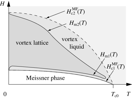
Figure 1: Schematic illustration of the phase diagram of type-II superconductors in the $(T,H)$ plane. In mean-field theory, vortices form the Abrikosov vortex lattice between the critical fields $H_{\rm c1}^{\rm MF}$ and $H_{\rm c2}^{\rm MF}$. Due to thermal fluctuations the vortex lattice is solid only between the melting fields $H_{\rm m1}$ and $H_{\rm m2}$ (dark shaded area) along which it melts into a vortex liquid.

Alternatively, one could start directly from the GL-Hamiltonian and study the fluctuation corrections in the vicinity of $H_{\rm c2}^{\rm MF}$ (see, e.g., [Lee and Shenoy 1972] (?), [Bray 1974] (?), [Thouless 1975] (?), [Ruggeri and Thouless 1976] (?), [Ruggeri 1979] (?), [Brézin et al. 1985] (?), [Affleck and Brézin 1985] (?), [Brézin et al. 1990a] (?), [Radzihovsky 1995b] (?)). As first observed by [Lee and Shenoy 1972] (?), the fluctuations in a $d$-dimensional superconductor in an external field are like those of a $(d-2)$-dimensional system in zero field, suggesting that the mean-field phase transition to an Abrikosov phase with ODLRO is destroyed by fluctuations in dimensions $d<d_{\rm cl}^{\rm ODLRO}=4$ (the upper critical dimension of the system is now $d_{\rm cu}^{\rm ODLRO}=6$). This somewhat surprising conclusion is in agreement with calculations of Moore (?, ?) and others ([Glazman and Koshelev 1991a] (?, ?), [Ikeda et al. 1992] (?)), who found the destruction of ODLRO by strong phase fluctuations below a lower critical dimension, $d\leq d_{\rm cl}^{\rm ODLRO}$, starting from the existence of a periodic solution, i.e. of a vortex lattice within the GL-theory.

Detailed considerations show that the lower critical dimension $d_{\rm cl}^{\rm ODLRO}=4$ for systems with screening and $d_{\rm cl}^{\rm ODLRO}=3$ for systems without screening (Moore ?, ?). Since the aforementioned calculations on fluctuation effects close to $H_{\rm c2}^{\rm MF}$ use the LLL approximation which usually neglects screening, it is clear that a simple dimensionality shift by 2 does not work here. Qualitatively, it is plausible that screening as an additional source of fluctuations increases $d_{\rm cl}^{\rm ODLRO}$. A similar effect is also observed for gauge glasses (see section 2.4). Quantitatively, the shift of $d_{\rm cl}^{\rm ODLRO}$ can be traced back to the strong dispersion of the tilt modulus for $k>\lambda^{-1}$ [Moore 1992]. (Note that the compression modulus does not affect the formation of ODLRO.) Breakdown of dimensionality reduction by 2 was also shown by [Radzihovsky and Balents 1996] (?) in a layered superconductor in a parallel field, where $d_{\rm cl}^{\rm ODLRO}=2.5$ but the upper critical dimension $d_{\rm cu}^{\rm ODLRO}=5$, and the vortex lattice is still stable in $d\geq 2$ dimensions.

ODLRO is conventionally defined by a non-vanishing limit of the gauge invariant pair correlation function

$$C_{2}({\bf r}_{1},{\bf r}_{2};\Gamma)=\langle\Psi({\bf r}_{1})\Psi^{*}({\bf r}_{2})e^{i(2\pi/\Phi_{0})\int_{\Gamma}d{\bf r}\cdot{\bf A}}\rangle$$ (2.24)

for $|{\bf r}_{1}-{\bf r}_{2}|\to\infty$. ($\langle\cdot\rangle$ denotes the average over thermal fluctuations.) Note that $C_{2}({\bf r}_{1},{\bf r}_{2};\Gamma)$ itself depends on the path $\Gamma$ between ${\bf r}_{1}$ and ${\bf r}_{2}$ along which the vector potential is integrated. The proposal of [Moore 1992] (?) to keep only the longitudinal component of ${\bf A}$ to make $C_{2}$ path independent but preserve its gauge invariance corresponds in the London gauge to the complete neglection of the phase factor $e^{i(2\pi/\Phi_{0})\int_{\Gamma}d{\bf r}\cdot{\bf A}}$ in equation (2.24).

In fact, a non-vanishing asymptotic expression for $C_{2}({\bf r}_{1},{\bf r}_{2};\Gamma)$ if $|{\bf r}_{1}-{\bf r}_{2}|\to\infty$ may not be the appropriate definition for the existence of long-range order in cases in which topological defects are forced into the system by external boundary conditions or (as in type-II superconductors) external fields. The most simple counter example is an Ising magnet below $T_{c}$ with anti-periodic boundary conditions, which force a domain wall into the system. Wall fluctuations will then suppress magnetic correlations. The loss of ODLRO due to thermal fluctuations in type-II superconductors – if concluded from the asymptotic behaviour of $C_{2}$ – is related to the fact that phase fluctuations $\delta\phi({\bf r})$ of the order parameter are related to (shear) distortions ${\bf u}({\bf r})$ of the vortex-line lattice via [Moore 1992, Ikeda et al. 1992, O’Neill and Moore 1993, Baym 1995]

$$\delta\phi({\bf k})=\frac{2\pi i}{a^{2}}\frac{k_{x}u_{y}({\bf k})-k_{y}u_{x}({\bf k})}{k^{2}}.$$ (2.25)

Here we used the Fourier transforms $\delta\phi({\bf k})$ and ${\bf u}({\bf k})$ of the fields $\delta\phi({\bf r})=\phi({\bf r})-\phi_{0}({\bf r})$ and ${\bf u}({\bf r})$ and ${\bf k}=(k_{x},k_{y},{\bf k}_{\parallel})$. $\phi_{0}({\bf r})$ denotes the phase in the ground state. Note that equation (2.25) is not in contradiction to equation (2.10) since ${\mbox{\boldmath${{\nabla}}$}}^{2}\phi_{\rm v}({\bf r})\neq 0$ only at the vortex sites. Equation (2.25) implies that on large length scales phase fluctuations are amplified displacement fluctuations of the vortex-line lattice. Destruction of ODLRO below $d=4$ dimensions does not mean however – this is the point of view we will take here – the absence of any ordered phase. This can be concluded from the London approximation (2.15): Expressing ${\bf B}({\bf r})$ with the help of (2.14) in terms of the vortex degrees of freedom, the only phase fluctuations left are spin-wave like which lead to a destruction of conventional long-range order only in $d\leq 2$ dimensions. The energy of the vortex lattice can be approximated at low $T$ by an elastic Hamiltonian (2.16) which may be supplemented by a contribution from dislocations. For $d\geq 3$ such a system shows a phase with translational long-range order (TLRO) for $H_{\rm m1}(T)<H<H_{\rm m2}(T)$. (In $d=2$ dimensions, elastic fluctuations reduce the order to quasi-TLRO characterized by a power-law decay of correlations.) In the elastic description, which we will use in most parts of this review, the appropriate order parameter for TLRO is

$$\psi_{{\bf Q}}({\bf r})=e^{i{\bf Q}\cdot{\bf u}({\bf r})}$$ (2.26)

with $\langle\psi_{{\bf Q}}({\bf r})\rangle\not=0$ in the Abrikosov phase. ${\bf Q}$ denotes a reciprocal lattice vector of the Abrikosov lattice. From this point of view the loss of ODLRO has no physical significance. $C_{2}$ is therefore not the appropriate quantity to define order. This conclusion is in agreement with a number of numerical investigations in which a clear indication for a transition to an ordered phase was seen in two and three dimensions. [Hu and MacDonald 1993] (?) and [Kato and Nagaosa 1993a] (?) have considered the pair correlation function of the superfluid density

$$C_{4}({\bf r}_{1},{\bf r}_{2})=\langle|\Psi({\bf r}_{1})|^{2}|\Psi({\bf r}_{2})|^{2}\rangle.$$ (2.27)

Using the LLL approximation both groups found a clear indication for a first order melting transition in $d=2$. Their work was extended by [Šašik and Stroud 1993] (?, ?) to three-dimensional systems. They considered the helicity modulus

$$\gamma_{\alpha\beta}({\bf r},{\bf r}^{\prime})=\left.\frac{\partial\langle j_{\alpha}({\bf r})\rangle}{\partial A^{\prime}_{\beta}({\bf r}^{\prime})}\right|_{{\bf A}^{\prime}={\bf 0}}=\frac{c}{4\pi\lambda^{2}}\delta({\bf r}-{\bf r}^{\prime})\delta_{\alpha\beta}-\frac{1}{cT}\langle j_{\alpha}({\bf r})j_{\beta}({\bf r}^{\prime})\rangle_{c},$$ (2.28)

where ${\bf A}^{\prime}$ is an additional vector potential and ${\bf j}$ the current density. In the LLL (where $\lambda\to\infty$) they found a rapid increase of $\gamma_{zz}$ at the freezing temperature, indicating the formation of a vortex-line lattice. [Šašik et al. 1995] (?) have subsequently shown that the vortex liquid-to-solid transition is not accompanied by a divergence of the correlation length for phase coherence. In their simulation $C_{2}$ decays exponentially even in the solid phase in agreement with the predictions of [Moore 1992] (?), [Ikeda et al. 1992] (?), and [Baym 1995] (?).

It has to be mentioned, however, that the point of view we adopt in this article – namely that the loss of ODLRO does not rule out the existence of a vortex lattice – is not shared by all authors. In particular Moore (?, ?, ?) argues that there is no mixed phase in type-II superconductors at finite temperatures. The observed effects in the behaviour of resistance and magnetization are explained as cross-over phenomena which would disappear in the thermodynamic limit. Moreover, the vortex lattices found in the Monte-Carlo simulations mentioned before is considered to be an artifact produced by the quasi-periodic boundary conditions used in these simulations. Moore and co-workers [O’Neill and Moore 1992, O’Neill and Moore 1993, Lee and Moore 1994, Dodgson and Moore 1997, Kienappel and Moore 1999, Moore and Pérez-Garrido 1999] have tried in their own Monte-Carlo simulations to avoid these effects (which they consider to be crucial) by placing the two-dimensional superconductor on the surface of a sphere. In their studies no freezing transition to a vortex-lattice state was observed. It should however be mentioned that zero-energy modes connected with the rigid rotations of the film on the sphere and disclinations arising from topological constraints for a triangular lattice on the sphere may obscure the transition.

To conclude: Although the absence of ODLRO at finite temperatures in the mixed phase of type-II superconductors (see, e.g., [Houghton et al. 1990]) and its consequences for the existence of a vortex lattice are still under debate, the most simple scenario is the existence of a vortex lattice in the absence of ODLRO below $d=4$ dimensions. The continuous translational invariance of the system is reduced to finite translations by lattice vectors ${\bf X}$ of the Abrikosov lattice. In contrast to ODLRO, the lower critical dimension for TLRO in pure systems is $d_{\rm cl}^{\rm TLRO}=2$.

Since the critical regime is enlarged in a non-zero external field (in $d=3$) to [Ikeda et al. 1989]

$$\frac{T_{\rm c}(H)-T}{T_{\rm c}(H)}\lesssim{\rm Gi}^{1/3}\left(\frac{H_{\rm c2}^{\rm MF}(T)}{H_{\rm c2}^{\rm MF}(0)}\right)^{2/3}$$ (2.29)

with respect to the zero-field critical region, but is still too small to describe the difference between ${H_{\rm c2}^{\rm MF}(T)}$ and the melting line, [Feigelman et al. 1993] (?) have argued that between the Abrikosov lattice and the normal phase there may be an intermediate liquid phase which still shows longitudinal superconductivity. We will not follow this idea here since more recent extensive simulations show only a single transition between the Abrikosov and the normal phase [Hu et al. 1997, Hu et al. 1998, Nguyen and Sudbø 1998, Nordborg and Blatter 1997, Nordborg and Blatter 1998, Olsson and Teitel 1999], although further proposals for an intermediate phase were made recently [Tešanović 1999, Nguyen and Sudbø 1999].

In the rest of this article we will ignore the existence of these exotic phases in pure superconductors (although their existence cannot be ruled out completely), but concentrate instead on the influence of randomly distributed frozen impurities on the vortex-line lattice phase. The impurities will be assumed to be completely uncorrelated as already mentioned in the introduction. Columnar or planar defects lead to very different physics (for a recent review on the so-called Bose glass, see [Täuber and Nelson 1997] (?) and references therein) and will not be discussed in this paper.

2.4 The influence of disorder

Disorder can be introduced in the Ginzburg-Landau model (2.1) by assuming small random contributions to all parameters which characterize the system, i.e. $\alpha,\;\beta,\;m$ and ${\bf H}$. We will restrict ourselves here to the case of systems with random mean-field transition temperature $T_{\rm c0}$, i.e. we substitute

$$T_{\rm c0}\to T_{\rm c0}+\delta T_{\rm c0}({\bf r})$$ (2.30)

with

$$\overline{\delta T_{\rm c0}({\bf r})\,\delta T_{\rm c0}({\bf r}^{\prime})}=\xi^{2}\,\delta_{\xi}({\bf r}-{\bf r}^{\prime})\,\delta T_{\rm c0}^{2}$$ (2.31)

where the overbar denotes the disorder average and $\delta_{\xi}({\bf r})$ is a $\delta$-function of widths $\xi$.

In mean-field theory, a randomness in $T_{\rm c0}$ would correspond to a smearing out of the transition. However, as first shown by [Khmelnitskii 1975] (?), thermal fluctuations permit the occurrence of a sharp phase transition. According to the so-called Harris criterion [Harris 1974] weak randomness does not change the critical behaviour if the exponent of the specific heat of the pure system $\alpha_{\rm pure}$ is negative, or, equivalently, if the correlation length exponent $\nu_{\rm pure}$ obeys $\nu>2/d$. Since for the $XY$-model in three dimensions $\alpha$ is negative [Lipa et al. 1996], the zero-field critical behaviour for type-II superconductors should be unchanged in the outer critical region. This would also apply in case that behaviour of the pure system in the inner critical region is also of (inverted) $XY$-type. On the contrary, for type-I superconductors it was shown by [Boyanovsky and Cardy 1982] (?) that a sufficiently large amount of disorder may convert the first order transition into a second order one.

If an external field is applied, the situation is quite different. Because of the problems connected with ODLRO even in pure systems, which were discussed in the previous chapter, it seems to be expedient to first consider the influence of disorder on the structural properties of the mixed phase.

Inside the Abrikosov phase, disorder leads to a destruction of translational long-range order as first shown by [Larkin 1970] (?). This follows from the fact that a randomness in the local value of $T_{c}({\bf r})$ leads to a random potential acting on the vortices. The specific form of the resulting coupling of the disorder to the vortex displacements will be given in the following chapters. The disorder averaged order parameter $\overline{\langle e^{i{\bf Q}\cdot{\bf u}}\rangle}$ for TLRO vanishes since disorder leads to diverging displacement ${\bf u}$ in the limit of large system sizes. However, it will be shown below that the correlation function

$$S({\bf Q},{\bf r})=\overline{\langle e^{i{\bf Q}\cdot[{\bf u}({\bf r})-{\bf u}(\bf 0)]}\rangle}$$ (2.32)

may still obey an algebraic decay, which shows up in Bragg peaks in the structure factor (Giamarchi and Le Doussal ?, ?, [Emig et al. 1999]). Moreover, in analogy with spin glass theory (see [Binder and Young 1986] (?)) one may consider the positional glass correlation function

$$S_{\rm PG}({\bf Q},{\bf r})=\overline{\Big{|}\langle e^{i{\bf Q}\cdot[{\bf u}({\bf r})-{\bf u}(\bf 0)]}\rangle\Big{|}^{2}}$$ (2.33)

as another signature of the existence of some residual, ‘glassy’ order of the Abrikosov lattice. Below we will call a system a positional vortex glass if $S_{\rm PG}({\bf Q},{\bf r})$ decays not faster than a power law for $|{\bf r}|\to\infty$. For $T\to 0$, $S_{\rm PG}({\bf Q},{\bf r})$ approaches one. At non-zero temperature, (2.33) measures the strength of thermal fluctuations of the vortex lines around the ground state. Two limiting cases seem to be conceivable: If the disorder acts effectively as a random force on the vortex lines, then the thermal fluctuations around the disordered ground state are identical to those of the pure system. In this case (2.33) is non-zero above $d=2$ dimensions. In the opposite case of very strong pinning the vortex lines can be considered to fluctuate thermally in a kind of narrow parabolic potential and (2.33) may be finite even in $d<2$. The relevance of these structural correlation functions for the glassy behaviour of the mixed phase will be further discussed in the following chapters.

A complementary discussion of the glassy behaviour was proposed by M. P. A. Fisher (?) and [Fisher et al. 1991a] (?). These authors use the correlation function for ODLRO as the starting point. Clearly, because of the relation (2.25), $\overline{\langle\Psi({\bf r})\Psi^{\ast}({\bf 0})\rangle}$ will vanish for $r\to\infty$ in $d<4$ dimensions. In analogy to spin glasses they therefore introduce the correlation function for phase-coherent vortex-glass order (using the London gauge ${\mbox{\boldmath${{\nabla}}$}}\cdot{\bf A}=0$):

$$C_{\rm VG}({\bf r})=\overline{\big{|}\big{<}\Psi^{\ast}({\bf r})\Psi({\bf 0})\big{>}\big{|}^{2}}\,.$$ (2.34)

It is instructive to consider (2.34) in the London limit where $C_{\rm VG}({\bf r})\approx|\Psi_{0}|^{2}\overline{|\langle e^{i[\delta\phi({\bf r})-\delta\phi({\bf 0})]}\rangle|^{2}}$. $\delta\phi({\bf r})$ describes the fluctuations around the ground state pattern $\phi_{0}({\bf r})$. If the disorder is of random-force type, according to (2.25) thermal fluctuations should destroy $C_{\rm VG}({\bf r})$ below $d=4$. On the other hand for thermal fluctuations in a parabolic potential around the ground state, $C_{\rm VG}({\bf r})$ should be finite.

[Dorsey et al. 1992] (?) and Ikeda (?, ?) have calculated the vortex glass susceptibility $\chi_{\rm VG}=\int d^{d}r\ C_{\rm VG}({\bf r})$ for a GL-Model with random transition temperature in the LLL approximation. [Dorsey et al. 1992] (?) found in a mean-field calculation a second-order transition with a diverging vortex-glass susceptibility by approaching the vortex-glass transition temperature $T_{\rm g}(H)$, which is slightly below $T_{\rm c2}(H)$. In mean-field theory, the vortex-glass correlation length $\xi_{\rm VG}$ diverges with a mean-field exponent $\nu^{\rm MF}_{\rm VG}=1/2$. From this one can expect the existence of a non-zero limit of $C_{\rm VG}({\bf r})$ for $|{\bf r}|\to\infty$ below $T_{\rm g}(H)$. Taking critical fluctuations into account, which can be done within a $d=6-\epsilon$ expansion, the model is found to be in the some universality class as the Ising spin glass. In particular, the dynamical critical exponent is found to be $z=2(2-\eta)$, where $\eta\simeq-\epsilon/6$. It should be observed that a similarity between the Ising spin glass and vortex glasses was also mentioned for so-called gauge-glass models (see [Huse and Seung 1990] (?)). On the other hand, the results of [Dorsey et al. 1992] (?) and Ikeda (?, ?) – if applied to $d=3$ dimensions – cannot be so easily reconciled with the findings from the elastic description of a vortex lattice in a random potential. As we will discuss in chapter 6, the vortex lattice exhibits indeed a glassy phase (the Bragg glass) for $2<d\leq 4$, in which the correlation function $C_{\rm VG}({\bf r})$, if calculated to lowest order in $\epsilon=4-d$, vanishes for large $|{\bf r}|$ exponentially. The reason for this decay consists in the strong thermal fluctuations of the phases around the (distorted) ground state. To order $\epsilon$, these phase fluctuations are only weakly suppressed by disorder and hence $C_{\rm VG}({\bf r})$ decays exponentially. However, higher order terms in $\epsilon$ may still change this result. In principle, there could be two glassy phases, which show a non-vanishing $S_{\rm PG}({\bf Q},{\bf r})$ and $C_{\rm VG}$, respectively. For the moment we consider it to be more likely that there is only one glassy phase and the discrepancy between the results follows from the use of different approximations valid in $d=6-\epsilon$ and $d=4-\epsilon$ dimensions, respectively.

So far we assumed that the disorder is weak. On the other hand gauge-glass like models were proposed for the description of granular superconductors or systems with strong disorder [Ebner and Stroud 1985, John and Lubensky 1986]. Each superconducting grain of centre position ${\bf r}_{i}$ is described by the phase $\phi_{i}$ of the order parameter which is assumed to be constant within a grain. The Hamiltonian then reads (see e.g. [Wengel and Young 1996] (?))

$${\cal H}=-J\sum\limits_{<ij>}\cos{(\phi_{i}-\phi_{j}-A_{ij}-\lambda_{0}^{-1}a_{ij})}+\frac{1}{2}\sum\limits_{\Box}({\mbox{\boldmath${{\nabla}}$}}\wedge{\bf a})^{2}\,,$$ (2.35)

where $a_{ij}=\int\limits_{{\bf r}_{j}}^{{\bf r}_{i}}{\bf a}({\bf r})\,d{\bf r}$. $\sum\limits_{<ij>}$ is the sum of all nearest neighbors of a cubic lattice and $\sum\limits_{\Box}$ is the sum over all plaquettes. ${\bf a}$ denotes the fluctuations of the vector potential which are limited by the bare screening length $\lambda_{0}$. The influence of the external field as well as the contribution from randomness are assumed to be included in the $A_{ij}$ which are taken to be independent random variables with a distribution between 0 and $2\pi$. A detailed discussion of the relation between the vortex glass (the expression is here understood in the sense that it describes the glassy phase of an impure type-II superconductor in an external field) and gauge glasses is given in [Blatter et al. 1994] (?). The model (2.35) is in particular isotropic in contrast to the GL-Hamiltonian which shows a pronounced anisotropy due to the presence of the external field ${\bf H}$. In addition, the disorder of the gauge glass has a nature which is completely different from the one in equation (2.30). The first one couples to the vortices via the phase of the order parameter, while the latter one couples only via the amplitude. As a consequence, the gauge-glass disorder distorts the vortices much more than local variations of $T_{\rm c0}$.

For $\lambda_{0}\to\infty$, i.e. in the absence of screening, the gauge glass was investigated numerically by a number of authors (see [Fisher et al. 1991b] (?), [Gingras 1992] (?), [Cieplak et al. 1991] (?), [Reger et al. 1991] (?), [Cieplak et al. 1992] (?), [Hyman et al. 1995] (?), [Maucourt and Grempel 1998] (?), [Kosterlitz and Akino 1998] (?), [Olson and Young 1999] (?)). While in two dimensions a transition to a glass phase is found to be only at $T=0$, this transition takes place at finite temperatures in three dimensions. [Huse and Seung 1990] (?) found at the transition a diverging gauge-glass susceptibility

$$\chi_{\rm GG}=\sum\limits_{j}C_{\rm GG}({\bf r}_{i}-{\bf r}_{j})\,,$$ (2.36)

where $C_{\rm GG}$, in analogy with (2.34), denotes the gauge glass correlation function

$$C_{\rm GG}({\bf r}_{i}-{\bf r}_{j})=\overline{\big{|}\langle e^{i(\phi_{i}-\phi_{j})}\rangle\big{|}^{2}}\,.$$ (2.37)

The divergence of $\chi_{\rm GG}$ may signal the transition to a phase with non-zero limit of $C_{\rm GG}({\bf r})$ for $|{\bf r}|\to\infty$. If one assumes (2.34) as the definition of vortex glass order, then the gauge glass would be a vortex glass.

More recently, the case of a finite $\lambda_{0}$ was considered [Bokil and Young 1995, Wengel and Young 1996, Wengel and Young 1997, Kisker and Rieger 1998]. It turns out that screening seems to destroy the gauge glass transition in three dimensions. More recently [Kawamura 1999] (?) and [Pfeiffer and Rieger 1999] (?) have attempted to include the effect of anisotropy into the gauge glass model by assuming an extra contribution to $A_{ij}$ arising from the external field. However, also in this case no finite temperature glass transition was found.

3 Directed elastic manifolds in a random potential

In the course of this article we will restrict our consideration of fluctuations to vortices and we will ignore other independent fluctuations such as those of the condensate amplitude or of the magnetic field. Vortices will be treated within the London picture, where vortex lines are represented as string-like objects. For low temperatures and weak disorder the vortex lines will fluctuate only weakly around the ground state of the vortex-line lattice (VLL), the Abrikosov lattice, where all lines are directed along the magnetic field.

Before we analyze the VLL as an ensemble of vortex lines in its full complexity it is instructive to study a single vortex line. In general, a vortex can be characterized by two dimensions which depend on the physical realization under consideration: the ‘internal’ dimension $D$ of the vortex considered as a ‘directed manifold’, and the number $N$ of its displacement components. For example, a vortex line in a bulk superconductor has $(D,N)=(1,2)$, a single vortex line in a superconducting film has $(D,N)=(1,1)$, and a point vortex in a film corresponds to $(D,N)=(0,2)$. This concept of elastic manifolds also applies to other physical systems such as interfaces between magnetic domains, for which $(D,N)=(2,1)$. In all these examples the spatial dimension of the system is $d=D+N$, since displacements are possible only in directions orthogonal to the ${\bf z}$ direction(s) along which the manifold is spanned.

It is worthwhile to mention at this point that the analysis of random manifolds applies not only to single vortex lines, but to a certain extent (i.e., within a regime of length scales) also to vortex line lattices. For example, the VLL in a weakly disordered bulk superconductor resembles over a large range of length scales an elastic manifold with $(D,N)=(3,2)$. In this case, where the elastic manifold is spanned in all spatial dimensions including the displacement directions, $d=D$. Nevertheless, there is a fundamental difference between manifolds and VLLs, which is crucial for the physics on large scales: VLLs have a periodic structure in contrast to manifolds.

To parameterize vortex conformations, we use the $D$-dimensional coordinate ${\bf z}$ along the direction of the magnetic field and a $N$-dimensional coordinate ${\bf x}\equiv{\bf x}({\bf z})$ in transverse directions, see figure 2.

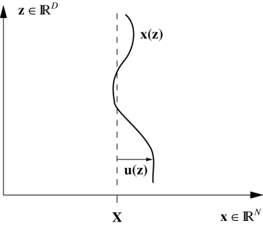
Figure 2: Illustration of the manifold coordinate system. The manifold conformation (solid line) is described by the $N$-component vector ${\bf x}$ as a function of the $D$-dimensional coordinate ${\bf z}$. The displacement ${\bf u}({\bf z})\equiv{\bf x}({\bf z})-{\bf X}$ is defined with respect to a flat reference position ${\bf X}$ (dashed line).

In this chapter we are mainly interested in qualitative aspects of vortex fluctuations in the presence of disorder. To this end we describe the elastic energy of a vortex line, which arises from the kinetic energy of the supercurrents and the magnetic field energy, in a harmonic approximation (i.e., we keep only terms of second order in the displacement) and we ignore non-localities or possible anisotropies in the elastic stiffness constant $\varepsilon_{\parallel}$. Then the elastic energy can be written as

$${\cal H}_{\rm el} = \int d^{D}z\ \frac{\varepsilon_{\parallel}}{2}({\mbox{\boldmath${{\nabla}}$}}_{\parallel}{\bf x})^{2}.$$ (3.1)

Therein the gradient ${\mbox{\boldmath${{\nabla}}$}}_{\parallel}\equiv(\frac{\partial}{\partial z_{1}},\dots,\frac{\partial}{\partial z_{D}})$ acts along the longitudinal ${\bf z}$ directions.

Pinning of vortex lines due to the presence of impurities, grain boundaries etc. can be described by a potential $V({\bf x},{\bf z})$ which is ‘quenched’, i.e., frozen on the relevant time scale for vortex fluctuations. It yields a contribution

$${\cal H}_{\rm pin} = \int d^{D}z\ V({\bf x}({\bf z}),{\bf z})$$ (3.2)

to the total energy ${\cal H}={\cal H}_{\rm el}+{\cal H}_{\rm pin}$ of a vortex line. For simplicity, we will discuss here only point-like disorder. We will assume that this potential is Gaussian distributed with zero average and variance

$$\overline{V({\bf x},{\bf z})V({\bf x}^{\prime},{\bf z}^{\prime})} = \Delta({\bf x}-{\bf x}^{\prime})\delta({\bf z}-{\bf z}^{\prime}).$$ (3.3)

For simplicity we will restrict ourselves to disorder with short-ranged and isotropic correlations. Then the correlator $\Delta({\bf x})=\Delta(|{\bf x}|)$ can be characterized by its integral

$$\Delta_{0} \equiv \widehat{\Delta}({\bf 0})=\int d^{N}x\ \Delta({\bf x})$$ (3.4)

and a correlation length. Such a pinning potential can arise from point-like impurities that locally suppress the density of the superconducting condensate. The correlation length of the disorder then also coincides with the superconducting coherence length $\xi$. In principle, one can retain a finite correlation length in the ${\bf x}$ and ${\bf z}$ directions. However, it turns out a posteriori that – as long as the correlation length does not exceed the smallest scale of vortex conformations, which also is $\xi$ – correlations in ${\bf z}$ direction are irrelevant. Subsequently, we will often write $\Delta({\bf x})=\Delta_{0}\delta_{\xi}({\bf x})$, where $\delta_{\xi}$ denotes a Dirac delta-function smeared out on a scale $\xi$. For semi-quantitative purposes we occasionally use $\delta_{\xi}({\bf x})=(2\pi\xi^{2})^{-N/2}\exp(-{\bf x}^{2}/2\xi^{2})$. If we denote the pinning force of an individual impurity by $f_{\rm pin}$, then

$$\Delta_{0}\approx f_{\rm pin}^{2}n_{\rm i}^{(d)}\xi^{2N+2},$$ (3.5)

where $n_{\rm i}^{(d)}$ denotes the concentration of the impurities in the $d$ dimensional space.

Directed manifolds in disorder represent a paradigm for systems which are dominated by disorder. Since disorder leads to a frustrating competition between elastic and pinning energies, the structural order can be reduced substantially. In addition, the dynamics of the system can get extremely slow due to the quenched nature of disorder. Therefore such a system can be called a ‘glass’. Because of the simplicity of the manifold model, it plays a paradigmatic role for glassy systems and it allows the identification and the understanding of many characteristic features of a more complicated ‘vortex glass’.

3.1 Equilibrium properties

As we have seen, vortices in impure superconductors are a realization of ‘elastic manifolds’ in ‘random media’ which are paradigms for disordered systems. We now proceed to summarize briefly some key properties of the latter model system. For more detailed presentations about these random manifolds the reader is referred to review articles [Kardar 1994, Halpin-Healy and Zhang 1995, Lässig 1998a], in particular to [Blatter et al. 1994] (?) for a discussion in the context of vortex systems, as well as to [Nattermann and Rujan 1989] (?), [Belanger and Young 1991] (?) and [Young 1998] (?) in the context of disordered magnets. Subsequently we will focus our attention on the question, in what physical quantities ‘glassiness’ appears in these systems.

From a principal point of view, it is important to note that disorder breaks symmetries of the Hamiltonian of the pure system: translation invariance ${\bf x}({\bf z})\to{\bf x}({\bf z})+{\bf x}_{0}$ for a constant shift ${\bf x}_{0}$ of vortex lines, as well as an analogous rotation symmetry ${\bf x}({\bf z})\to{\mbox{\boldmath${{\cal R}}$}}\cdot{\bf x}({\bf z})$, for a rotation matrix ${{\cal R}}$. Therefore it is interesting to examine to what extent the physical state of the manifold in disorder actually reflects these broken symmetries, or whether these symmetries are restored due to thermal fluctuations.

3.1.1 Structure

One quantity of primary interest is the structure of the manifold in disorder which can be described in terms of displacement correlations. In the absence of disorder the vortex line has a flat ground state, ${\bf x}({\bf z})\equiv{\bf X}$ for all ${\bf z}$. Introducing the displacement ${\bf u}({\bf z})\equiv{\bf x}({\bf z})-{\bf X}$, shape fluctuations can be described by the relative displacement at points separated by a distance ${\bf z}-{\bf z}^{\prime}$ parallel to the magnetic field:

$$W({\bf z}-{\bf z}^{\prime}) \equiv \overline{\langle[{\bf u}({\bf z})-{\bf u}({\bf z}^{\prime})]^{2}\rangle}\sim|{\bf z}-{\bf z}^{\prime}|^{2\zeta}.$$ (3.6)

As already introduced above, $\langle\dots\rangle$ and $\overline{\dots\rule{0.0pt}{5.0pt}}$ denote the thermal and disorder average respectively. For large distances this quantity typically follows a power law with the roughness exponent $\zeta=\zeta(D,N)$. The manifold is called flat, if $W$ is finite for $|{\bf z}-{\bf z}^{\prime}|\to\infty$ (then the convergence of $W$ to its asymptotic value can be described by an exponent $\zeta<0$), whereas it is called rough if $W$ diverges (i.e., $\zeta\geq 0$, where $\zeta=0$ typically corresponds to $W({\bf z})\sim\ln^{\alpha}z$ with some power $\alpha$).

In the absence of disorder thermal fluctuations are described by an exponent

$$\zeta_{\rm th}=\frac{2-D}{2}.$$ (3.7)

The presence of disorder may increase the roughness and lead to a larger exponent $\zeta>\zeta_{\rm th}$. In particular, disorder always induces roughness in dimensions $2<D\leq 4$, as we will discuss in more detail below.

For $D<2N/(2+N)$ disorder is irrelevant at sufficiently high temperatures. There is a phase transition (see e.g. [Imbrie and Spencer 1988] (?) for the case $D=1$) between a low-temperature phase, where the manifold is disorder dominated and essentially shows the structure of the ground state, and a high-temperature phase, where the manifold is entropically driven out of the ground state and shows a structure as in the absence of disorder.

Actually, the physical situation can be more complicated if an upper critical dimension $N_{\rm cu}$ exists, above which the low-temperature phase is governed by the Gaussian exponents. The existence of an upper critical dimension is still controversial. [Moore et al. 1995] (?) argue for $N_{\rm cu}=4$ and [Lässig and Kinzelbach 1997] (?, ?) argue for $N_{\rm cu}\leq 4$ in $D=1$. We will not further discuss this possible complication here, assuming $N_{\rm cu}$ to be large enough such that the vortex systems of physical interest are not concerned.

For $D\geq 2N/(2+N)$ one can think of the manifold as having a unique disorder-dominated ground state. For all temperatures entropic effects are too weak to detach the manifold from its ground state.

3.1.1a Structural order parameter

In order to have a tool to quantify the structural order of the manifold, we introduce

$$\psi_{\bf k}({\bf z}) \equiv e^{i{\bf k}\cdot{\bf u}({\bf z})}$$ (3.8)

as order parameter. If the manifold performs only weak thermal fluctuations around its ground state, $\langle\psi_{\bf k}({\bf z})\rangle\neq 0$ and disorder actually breaks the translation symmetry of the manifold. Otherwise, if thermal fluctuations detach the manifold from its ground state, $\langle\psi_{\bf k}({\bf z})\rangle=0$. The correlation function of this order parameter,

$$S({\bf k},{\bf z}-{\bf z}^{\prime})\equiv\overline{\langle\psi_{\bf k}^{*}({\bf z})\psi_{\bf k}({\bf z}^{\prime})\rangle}\approx\exp\left(-\frac{1}{2}{\bf k}\cdot{\bf W}({\bf z}-{\bf z}^{\prime})\cdot{\bf k}\right),$$ (3.9)

is related to the displacement correlation

$$W_{\alpha\beta}({\bf z}-{\bf z}^{\prime}) \equiv \overline{\langle[u_{\alpha}({\bf z})-u_{\alpha}({\bf z}^{\prime})][u_{\beta}({\bf z})-u_{\beta}({\bf z}^{\prime})]\rangle}.$$ (3.10)

The function $W$, previously introduced in (3.6), is simply the trace of the matrix $W_{\alpha\beta}$. The approximate relation in (3.9) neglects higher cumulants of the displacement distribution and holds in general only for small displacement fluctuations. It even holds for large displacement fluctuations and actually is an identity, if the fluctuations of ${\bf u}$ have Gaussian distribution.

3.1.1b Perturbative analysis

A first qualitative insight into the relevance of disorder can be obtained from an elementary perturbative analysis. Such an analysis was performed originally by [Larkin 1970] (?) for vortex lattices and by [Efetov and Larkin 1977] (?) for the closely related charge-density waves.

In this approach the manifold (at $T=0$) is considered in an absolutely flat reference state ${\bf x}({\bf z})={\bf X}$, for which the pinning force ${\bf F}^{\rm pin}({\bf z})\equiv-{\mbox{\boldmath${{\nabla}}$}}_{\perp}V({\bf x}({\bf z}),{\bf z})$ is calculated. We denote by ${\mbox{\boldmath${{\nabla}}$}}_{\perp}\equiv(\frac{\partial}{\partial x_{1}},\dots,\frac{\partial}{\partial x_{N}})$ gradients in ${\bf x}$ directions in contrast to ${\mbox{\boldmath${{\nabla}}$}}_{\parallel}$ for ${\bf z}$ directions. From this force the disorder induced manifold displacement is obtained in linear response theory as $u_{\alpha}({\bf q})\equiv\int d^{D}z\ e^{-i{\bf q}\cdot{\bf z}}u_{\alpha}({\bf z})=G_{\alpha\beta}({\bf q})F^{\rm pin}_{\beta}({\bf q})$ using the response function

$$G_{\alpha\beta}({\bf z}-{\bf z}^{\prime})\equiv\frac{\delta u_{\alpha}({\bf z})}{\delta F^{\rm pin}_{\beta}({\bf z}^{\prime})},\quad\quad G_{\alpha\beta}({\bf q})=\frac{1}{\varepsilon_{\parallel}q^{2}}\delta_{\alpha\beta}$$ (3.11)

of the free manifold. Thus the displacement correlations are given in linear response by

$$\overline{\langle u_{\alpha}({\bf q})u_{\beta}(-{\bf q})\rangle}=G_{\alpha\gamma}({\bf q})\ \overline{F^{\rm pin}_{\gamma}({\bf q})F^{\rm pin}_{\delta}(-{\bf q})}\ G_{\beta\delta}(-{\bf q})=\frac{\Delta^{(2)}}{\varepsilon_{\parallel}^{2}q^{4}}\delta_{\alpha\beta},$$ (3.12)

where we introduced the variance of the pinning force $\Delta^{(2)}$ via

$$\Delta^{(2)}\delta_{\alpha\beta}\equiv-\partial_{\alpha}\partial_{\beta}\left.\Delta({\bf x})\right|_{{\bf x}={\bf 0}}.$$ (3.13)

Its value is related to the variance and correlation length of the pinning potential approximately through

$$\Delta^{(2)}=\frac{\Delta_{0}}{(2\pi)^{N/2}\xi^{2+N}}.$$ (3.14)

Here we have assumed a Gaussian form for $\Delta({\bf x})$.

The perturbative correlation function (3.12) is characterized by a roughness exponent

$$\zeta_{\rm rf}=\frac{4-D}{2},$$ (3.15)

which we refer to as the ‘random force’ value. This exponent characterizes the actual correlation function only on sufficiently small scales $|{\bf z}|\lesssim L_{\xi}$ below the Larkin length $L_{\xi}$ [Larkin 1970], since the perturbative treatment is justified only as long as $W({\bf z})\lesssim\xi^{2}$. The Larkin length can be estimated by equating the elastic energy $E_{\rm el}\approx\varepsilon_{\parallel}L_{\xi}^{D-2}\xi^{2}$ with the pinning energy in the random-force approximation $E_{\rm pin}\approx(L^{D}\xi^{2}\Delta^{(2)})^{1/2}$ as [Larkin 1970, Bruinsma and Aeppli 1984]

$$L_{\xi}\approx[\varepsilon_{\parallel}^{2}\xi^{2}/\Delta^{(2)}]^{1/\epsilon},$$ (3.16)

where $\epsilon\equiv 4-D$ (to be distinguished from $\varepsilon_{\parallel}$). From this rough analysis the manifold is found to be flat in $D>4$ (since $\zeta_{\rm rf}<0$), logarithmically rough in $D=4$ (with $\zeta_{\rm rf}=0$), and rough with an exponent $\zeta_{\rm rf}>0$ in $D<4$. Although the perturbative analysis can provide a good approximation only on small length scales $|{\bf z}|\lesssim L_{\xi}$ (however, in certain cases intermittency can be relevant on small scales [Bouchaud et al. 1995]), the roughness of the manifold in $D\leq 4$ persists in more sophisticated approaches (such as a self-consistent or renormalization-group analysis), which go beyond a perturbative approach.

Thus, a single vortex line ($D=1$) in a bulk superconductor ($d=3$), which is roughened by pure thermal fluctuations (cf. equation (3.7)), is also roughened by disorder at $T=0$. In contrast, a VLL in a bulk superconductor, which can be considered as a manifold with $D=d$, is not roughened by pure thermal fluctuations but by pinning.

3.1.1c Flory analysis

As already mentioned, the above perturbative analysis breaks down on length scales $|{\bf z}|\gtrsim L_{\xi}$ because perturbation theory does not adequately treat a system with many minima in the potential energy (for a pedagogical example see [Villain and Séméria 1983] (?)). Although perturbation theory could be continued to higher orders, it will never be able to describe the displacements on largest scales $|{\bf z}|\to\infty$, where the multi-stability (existence of many local minima) of the potential energy landscape is crucial.

For the further analysis it is convenient to start from the replica Hamiltonian [Edwards and Anderson 1975]

$${\cal H}_{n} = {\cal H}_{{\rm el},n}+{\cal H}_{{\rm pin},n}$$ (3.17)

$$= \sum_{a,b=1}^{n}\int d^{D}z\ \left\{\frac{\varepsilon_{\parallel}}{2}\delta^{ab}({\mbox{\boldmath${{\nabla}}$}}_{\bf z}{\bf u}^{a})^{2}-\frac{1}{2T}\Delta({\bf u}^{a}({\bf z})-{\bf u}^{b}({\bf z}))\right\},$$

which is obtained from replicating the original system $n$ times and performing a disorder average. Note that Greek lower indices denote transverse spatial components, whereas Roman upper indices denote replicas. The analysis of this Hamiltonian is highly non-trivial, since the displacement enters the argument of the disorder correlator $\Delta$. A dimensional analysis shows that $\Delta$ has to be retained in its full functional form and may not be represented by a truncated Taylor expansion in $D\leq 4$ [Balents and Fisher 1993].

Physically, the structure on large scales is determined by a competition between elastic and pinning energies. The Flory argument [Imry and Ma 1975, Kardar 1987, Nattermann 1987] allows one to obtain an improved value for the roughness exponent $\zeta$ by requiring both energy contributions to scale with the same exponent on large scales $|{\bf z}|$. To be more precise, we rescale ${\bf z}=L{\bf z}^{\prime}$ and ${\bf u}({\bf z})=L^{\zeta}{\bf u}^{\prime}({\bf z}^{\prime})$, where $L$ denotes the (variable) length scale on which we consider the system. Then ${\cal H}_{{\rm el},n}\sim L^{\theta}$ with an energy scaling exponent

$$\theta=2\zeta+D-2.$$ (3.18)

The fluctuations of ${\bf u}^{\prime}$ are determined by an effective temperature $T^{\prime}$, which has to be rescaled like the Hamiltonian,

$$T=T^{\prime}L^{\theta},$$ (3.19)

in order to keep the Boltzmann factor $e^{-{\cal H}/T}$ scale invariant.

In pure systems it is possible to achieve scale invariance not only of the Boltzmann factor $e^{-{\cal H}_{\rm el}/T}$ but of both $cH_{\rm el}$ and $T$ by the choice $\zeta=\zeta_{\rm th}\equiv\frac{2-D}{2}$ and $\theta_{\rm th}=0$.

At zero temperature, weak disorder is a relevant perturbation in $D\leq 4$. Since a short-ranged disorder correlator should essentially scale like an $N$-dimensional $\delta$-function, the replicated pinning energy scales as ${\cal H}_{\rm pin}/T\sim L^{D-N\zeta-2\theta}/{T^{\prime}}^{2}$. The exponent of the Boltzmann factor includes now two terms, which after rescaling behave as ${\cal H}_{\rm el}/T\sim{\cal H}_{\rm el}^{\prime}/T^{\prime}=O(1)$ and ${\cal H}_{\rm pin}/T=O(L^{D-N\zeta-2\theta})$. In the limit of vanishing temperatures, a finite width of the distribution of $\{{\bf u}^{\prime}\}$ is only possible if $L^{D-N\zeta-2\theta}=O(1)$, i.e., if

$$\zeta=\zeta_{\rm F}\equiv\frac{4-D}{4+N},$$ (3.20)

which implies $\theta=2\zeta+D-2=\frac{2+N}{4+N}(D-D_{N})$, where $D_{N}\equiv\frac{2N}{2+N}$. Although $\zeta_{\rm F}$ is an improvement over $\zeta_{\rm rf}$, this result is (in general) not exact, since the scaling behaviour of ${\cal H}_{\rm pin}$ was over-simplified.

On the other hand, at finite temperatures $e^{-{\cal H}_{{\rm pin},n}/T}$ is a relevant perturbation to the Boltzmann factor $e^{-{\cal H}_{\rm el}/T}$ if $D-N\zeta_{\rm th}-2\theta_{\rm th}>0$, i.e., for

$$D>D_{N}\equiv\frac{2N}{2+N},$$ (3.21)

which is equivalent to $\zeta_{\rm F}>\zeta_{\rm th}$. Note that $D_{N}<2$ for $N<\infty$ and $D_{\infty}=2$. From this observation we conclude that for $D<D_{N}$ weak disorder is irrelevant. Since on the other hand disorder will certainly become relevant if it is sufficiently strong, $\Delta>\Delta_{c}(T)$, one expects in this case a transition from an unpinned phase for weak disorder to a pinned phase at strong disorder (which is equivalent to a thermal depinning transition for increasing temperatures). Contrary to the result for $\zeta_{\rm F}$, which is an approximate expression for the true roughness exponent $\zeta$, the result for $D_{N}$ is exact.

3.1.1d Renormalization group analysis

The algebraic roughness (3.6) of the manifold means that it is scale invariant on large length scales. Hence it does not have a finite correlation length and the manifold can be considered as being in a critical state with $\zeta$ corresponding to a critical exponent. In analogy to ordinary critical phenomena, a renormalization group (RG) analysis is suitable to describe the large-scale features of the system going beyond perturbation theory and self-consistency arguments.

In $D\leq 4$ it is not possible to describe pinning by a finite set of parameters since $\zeta>0$ and a Taylor expansion of $\Delta({\bf u})$ would yield terms the relevance of which increases with increasing order of the expansion. Therefore one has to use a functional renormalization group analysis for the present problem, which was established by [Fisher 1986a] (?, ?) and [Balents and Fisher 1993] (?) to first order in $\epsilon\equiv 4-D$. On increasing length scales $L\propto e^{l}$ the system can be described by a renormalized temperature and disorder correlator, which flow according to [Fisher 1986a, Balents and Fisher 1993]:

$$\partial_{l}T = -\theta T,$$ (3.22a)

$$\partial_{l}\Delta({\bf u}) = (\epsilon-4\zeta)\Delta({\bf u})+\zeta u_{\alpha}\partial_{\alpha}\Delta({\bf u})$$ (3.22b)

$$+\frac{1}{2}\partial_{\alpha}\partial_{\beta}\Delta({\bf u})\partial_{\alpha}\partial_{\beta}\Delta({\bf u})-\partial_{\alpha}\partial_{\beta}\Delta({\bf u})\partial_{\alpha}\partial_{\beta}\Delta({\bf 0}).$$

Here we introduced a rescaled correlator $\Delta/c_{\Delta}\to\Delta$ with some non-universal constant $c_{\Delta}$ that depends on the short-scale cutoff and the stiffness constant $\varepsilon_{\parallel}$.

We will see that $\theta=D-2+2\zeta>0$ such that equation (3.22a) implies that the effective temperature vanishes on large scales. The system is therefore described asymptotically by a ‘zero temperature’ fixed point. The fixed-point correlator and exponent have to be determined numerically from equation (3.22b).

The actual value of the roughness exponent (‘random manifold’ value) can be represented introducing a correction factor $\nu(D,N)$ in the Flory expression (3.20),

$$\zeta_{\rm rm}=\frac{4-D}{4+\nu(D,N)N}.$$ (3.23)

In all known cases this correction factor lies in the range $0\leq\nu(D,N)\leq 1$. The findings of the functional RG analysis to order $\epsilon=4-D$ [Fisher 1986a, Balents and Fisher 1993] are equivalent to $\nu(4,1)\approx 0.800(3)$. It is interesting to note that the roughness can be determined exactly for special dimensions: $\nu(D,\infty)=1$, i.e., the Flory exponent becomes exact for an infinite number of displacement components [Mézard and Parisi 1990, Mézard and Parisi 1991], and $\nu(1,1)=0.5$ corresponding to $\zeta=\frac{2}{3}$ [Huse et al. 1985]. From a more involved field-theoretical self-consistency argument [Lässig 1998b] (?) obtains $\nu(1,2)=\frac{2}{5}$ corresponding to $\zeta=\frac{5}{8}$ and $\nu(1,3)=\frac{8}{21}$ corresponding to $\zeta=\frac{7}{12}$.

Remarkably, there is no renormalization of the elastic constant $\varepsilon_{\parallel}$ in the Hamiltonian. The renormalized elastic constant of the manifold can be determined from its response to tilt field $\mu^{*}_{i\alpha}$, which is coupled to the displacements through

$${\cal H}_{\mu}=-\int d^{D}z\ \mu^{*}_{i\alpha}\partial_{i}u_{\alpha}({\bf z}).$$ (3.24)

In the absence of a pinning potential a constant tilt field leads to a manifold displacement $u^{*}_{\alpha}({\bf z})=\mu^{*}_{i\alpha}z_{i}/\varepsilon_{\parallel}$ and to a change of the free energy by an amount

$$\overline{{\cal F}[{\mbox{\boldmath${{\mu^{*}}}$}}]}-\overline{{\cal F}[0]}=-\int d^{D}z\ \frac{1}{2\varepsilon_{\parallel}}{\mu^{*}_{i\alpha}}^{2}.$$ (3.25)

Even in the presence of the pinning potential with a stochastic translation symmetry, this identity holds exactly. This is due to a ‘statistical symmetry’ of the pinning energy under a transformation ${\bf u}({\bf z})\to{\bf u}^{\prime}({\bf z})={\bf u}({\bf z})+{\delta{\bf u}}({\bf z})$ for an arbitrary function ${\delta{\bf u}}({\bf z})$ [Goldschmidt and Schaub 1985, Schulz et al. 1988, Balents and Fisher 1993], provided disorder has a vanishing correlation length in ${\bf z}$ directions, as assumed in equation (3.3). In particular, the choice $\delta u_{\alpha}({\bf z})=\mu^{*}_{i\alpha}z_{i}/\varepsilon_{\parallel}$ transforms the pinning potential $V({\bf X}+{\bf u}({\bf z}),{\bf z})\to V({\bf X}+{\bf u}({\bf z})+\delta{\bf u}({\bf z}),{\bf z})=V^{\prime}({\bf X}+{\bf u}({\bf z}),{\bf z})$, which has the same statistical properties as the original potential. This stochastic symmetry is reflected most obviously by ${\cal H}_{{\rm pin},n}$ in equation (3.17), which is invariant under the transformation ${\bf u}^{a}({\bf z})\to{\bf u}^{a}({\bf z})+{\delta{\bf u}}({\bf z})$ that is identical in all replicas. The non-renormalization of $\varepsilon_{\parallel}$ follows directly from (3.25), since renormalized elastic constants are defined by

$$\frac{1}{\varepsilon_{\parallel}^{\rm eff}}=\frac{1}{ND}\frac{\partial}{\partial\mu^{*}_{i\alpha}}\overline{\langle\partial_{i}u_{\alpha}\rangle}=-\frac{1}{NDL^{D}}\frac{\partial^{2}}{\partial{\mu^{*}_{i\alpha}}^{2}}\overline{{\cal F}[{\mbox{\boldmath${{\mu^{*}}}$}}]},$$ (3.26)

the change of the free energy and the dependence of $\overline{{\cal F}}$ on $\mu$ is independent of disorder. Here $L^{D}=\int d^{D}z1$ is the system size.

If one starts from a disorder with a finite correlation length also in ${\bf z}$ direction, there will be a finite renormalization of the elastic constants due to fluctuations on these small length scales. Beyond this scale, the manifold behaves as for vanishing correlation length. Therefore the asymptotic behaviour on large scales (and in particular the roughness exponent) will not be affected by such correlations.

The roughness exponent is, however, sensitive to the behaviour of $\Delta({\bf x})$ on large scales, if this correlator is long ranged. Although this scenario is not of immediate interest for the present consideration of pinning by point like defects, it is realized, for example, for pinning of vortex lines by columnar defects or for magnetic domain walls with random fields. In this case (where $N=1$), $\Delta(x)-\Delta(0)\propto|x|$ and the roughness exponent has the ‘random-field’ value [Villain 1984, Grinstein and Fernandez 1984, Bruinsma and Aeppli 1984]

$$\zeta_{\rm rfi}=\frac{4-D}{3}.$$ (3.27)

Surprisingly, this exponent characterizes the manifold in the presence of a driving force at the depinning threshold, as we will discuss below.

3.1.1e Pinning vs. thermal fluctuations

In section 3.1.1d, we have described the structure in the disorder-dominated regime, for the ‘zero-temperature’ fixed point. Now we reconsider the effect of thermal fluctuations in the presence of disorder. For this purpose [Fisher and Huse 1991] (?) separated the displacement correlation function (3.6) into two contributions, the first one due to disorder

$$W_{\rm pin}({\bf z}-{\bf z}^{\prime})\equiv\overline{\langle{\bf u}({\bf z})-{\bf u}({\bf z}^{\prime})\rangle^{2}},$$ (3.28)

and a second one

$$W_{\rm th}({\bf z}-{\bf z}^{\prime}) \equiv W({\bf z}-{\bf z}^{\prime})-W_{\rm pin}({\bf z}-{\bf z}^{\prime})$$ (3.29)

$$= \overline{\langle[{\bf u}({\bf z})-{\bf u}({\bf z}^{\prime})-\langle{\bf u}({\bf z})-{\bf u}({\bf z}^{\prime})\rangle]^{2}\rangle}$$

$$\sim \frac{T}{\varepsilon_{\parallel}}|{\bf z}-{\bf z}^{\prime}|^{2-D}$$

describing thermal fluctuations. In the absence of disorder, $W_{\rm pin}({\bf z}-{\bf z}^{\prime})=0$.

In particular $W_{\rm th}$ is found to be independent of disorder due to the statistical symmetry [Schulz et al. 1988, Fisher and Huse 1991] already mentioned above. Thus $W_{\rm th}({\bf z})\sim|{\bf z}|^{2\zeta_{\rm th}}$ with the exponent (3.7). Consequently, $W_{\rm pin}({\bf z})\sim|{\bf z}|^{2\zeta_{\rm rm}}$ in the low-temperature phase, where $\zeta_{\rm rm}>\zeta_{\rm th}$.

It was argued [Fisher and Huse 1991, Hwa and Fisher 1994a, Kinzelbach and Lässig 1995] that the manifold would have (with probability 1) a unique ground state. Then $W_{\rm pin}$ essentially characterizes the ground state of the manifold [Nattermann 1985a, Huse and Henley 1985] and $\zeta_{\rm rm}$ would be the roughness exponent thereof. However, a small fraction of samples (or, small areas within a sample) will have nearly degenerate excited states with large displacements relative to the ground state. Although such excitations are rare, due to the large displacements they can dominate several disorder-averaged thermodynamic quantities [Nattermann 1988, Hwa and Fisher 1994a]. In particular, these rare fluctuations are responsible for the growth of the thermal width $W_{\rm th}$ in $D\leq 2$. Although $W_{\rm th}$ shows exactly the same behaviour as in the absence of disorder, it is important to emphasize that the distribution of thermal fluctuations is highly non-Gaussian [Fisher and Huse 1991, Hwa and Fisher 1994a].

For $D>2$ thermal fluctuations have only a finite width and the equilibrium state of the manifold globally reflects the ground state. The broken translation of the Hamiltonian are reflected by the equilibrium state of the manifold.

In summary, the structure of elastic manifolds in weak disorder strongly depends on its dimensionalities and shows the following behaviour (see also figure 3):

• For $D>4$ the manifold is flat ($\zeta<0$) at all temperatures provided disorder is weak. Sufficiently strong disorder will always induce roughness.

• For $2<D\leq 4$ disorder roughens the manifold ($\zeta=\zeta_{\rm rm}$) at all temperatures. The manifold stays close to its ground state; the second moment of thermal displacements is finite.

• For $2\geq D\geq D_{N}=2N/(2+N)$ disorder still roughens the manifold ($\zeta=\zeta_{\rm rm}$) at all temperatures. Now also the second moment of thermal displacements is infinite.

• For $D<D_{N}$ and sufficiently high temperatures, the manifold is entropically driven out of the ground state and shows a structure similar to that in the absence of disorder ($\zeta=\zeta_{\rm th}$). However, there is also a low-temperature phase where disorder is relevant [Cook and Derrida 1989]. In other terms, the manifold shows a temperature-driven depinning transition at a finite temperature.

For more details, the interested reader is referred to [Halpin-Healy and Zhang 1995] (?) and [Lässig 1998a] (?).

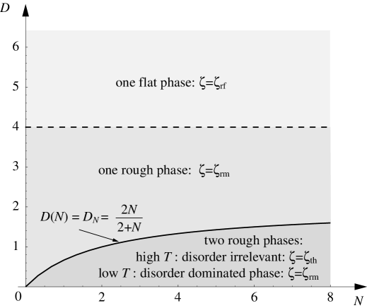
Figure 3: Illustration of the relevance of disorder for the roughness of the manifold in the $(D,N)$-plane (as described in the text).

3.1.2 Thermodynamics

So far we have described the relevance of disorder for the structure of the manifold. In particular, the roughness is qualitatively increased in the disorder dominated phases. Could such an increased roughness be taken as an unambiguous sign for glassiness of the state? To understand this problem better, we study the possibility of anomalous scaling properties of thermodynamic quantities such as energy, entropy, and free energy.

Since the elastic energy and the pinning energy are local quantities, energy, entropy, and free energy scale extensively with the system size $L$:

$$\overline{\cal E}\sim L^{D},\quad\overline{\cal S}\sim L^{D},\quad\overline{\cal F}\sim L^{D}.$$ (3.30)

Due to the randomness of pinning there are important sample-to-sample fluctuations with a scaling (for $T>0$)

$$\overline{(\Delta{\cal E})^{2}}\sim L^{D},\quad\overline{(\Delta{\cal S})^{2}}\sim L^{D},\quad\overline{(\Delta{\cal F})^{2}}\sim L^{2\theta},\quad$$ (3.31)

which has been confirmed numerically [Fisher and Huse 1991]. Here $\theta$ is again the energy scaling exponent (3.18). The fluctuations of $\Delta{\cal E}\equiv{\cal E}-\overline{\cal E}$ and $\Delta{\cal S}\equiv{\cal S}-\overline{\cal S}$ are normal and dominated by fluctuations on small scales: each sub-volume of the size $L_{\xi}^{D}$ contributes independently. However, the fluctuations of $\Delta{\cal F}\equiv{\cal F}-\overline{\cal F}$ are anomalous and governed by large-scale contributions. Clearly, for $T\to 0$ there exists a diverging length scale below which the fluctuations of $\Delta{\cal E}$ scale as those of $\Delta{\cal F}$.

In thermodynamic equilibrium the manifold minimizes its free energy. Therefore energy and entropy are not minimized independently, their leading order cancels (at $T>0$), and the free energy fluctuations can be smaller than those of the energy. One expects $\theta\leq\frac{D}{2}$ in all dimensions, which corresponds to $\zeta\leq\frac{4-D}{4}$ i.e., $\nu(D,N)\geq 0$ in equation (3.23). Indeed, the exponent $\zeta_{\rm IM}=(4-d)/4$ follows from an Imry-Ma type argument [Nattermann 1985a] and is considered to be an upper bound for $\zeta_{\rm rm}$ in random-bond systems [Fisher 1993]. At strictly zero temperature ${\cal E}={\cal F}$ and both quantities must scale in the same way, $\Delta{\cal E}=\Delta{\cal F}\sim L^{\theta}$. Therefore temperature plays a crucial role, although it seems to be irrelevant in the flow equation (3.22a). This is because temperature is a dangerously irrelevant variable [Fisher 1986b]. In very rare samples there are excited states which are nearly degenerate with the ground state but which deviate from it by large displacements. Such rare but large fluctuations still give dominant contributions to many thermodynamic disorder-averaged thermodynamic properties, for a more detailed discussion see [Fisher and Huse 1991] (?) and [Hwa and Fisher 1994a] (?).

3.1.3 Susceptibility

In order to find an unambiguous signature of glassy phases, [Hwa and Fisher 1994b] (?) proposed to examine the susceptibility of the system with respect to a tilt field. Although in this section we are dealing with directed manifolds, we establish the analogous susceptibility for these simpler systems and show how it is related to the displacement correlation functions discussed above.

For simplicity we restrict the discussion of susceptibilities to $N=1$; the general case $N>1$ follows from a straightforward generalization. We couple the manifold to an inhomogeneous tilt field ${\mbox{\boldmath${{\mu}}$}({\bf z})}$ via an additional energy contribution as in (3.24),

$${\cal H}_{\mu}=-\int d^{D}z\ [{\mbox{\boldmath${{\mu^{*}}}$}}+{\mbox{\boldmath${{\mu}}$}}({\bf z})]\cdot{\mbox{\boldmath${{\nabla}}$}}_{\parallel}u({\bf z}).$$ (3.32)

As in section 3.1.1d, ${{\mu^{*}}}$ is a constant field applied to measure the tilt response of the system.

The system

$${\cal H}^{\prime} = {\cal H}_{\rm el}+{\cal H}_{\mu}$$ (3.33)

$$= \int d^{D}z\left\{\frac{\varepsilon_{\parallel}}{2}\left({\mbox{\boldmath${{\nabla}}$}}_{\parallel}u-\frac{1}{\varepsilon_{\parallel}}[{\mbox{\boldmath${{\mu^{*}}}$}}+{\mbox{\boldmath${{\mu}}$}}]\right)^{2}-\frac{1}{2\varepsilon_{\parallel}}{[{\mbox{\boldmath${{\mu^{*}}}$}}+{\mbox{\boldmath${{\mu}}$}}]^{2}}\right\},$$

without random potential $V$ but with a random tilt ${\mbox{\boldmath${{\mu}}$}}({\bf z})$, has a ground state $u^{*}({\bf z})$ which couples only to the longitudinal part ${\mbox{\boldmath${{\mu}}$}}_{L}$ of the tilt field and which is determined by ${\mbox{\boldmath${{\mu^{*}}}$}}+{\mbox{\boldmath${{\mu}}$}}({\bf z})=\varepsilon_{\parallel}{\mbox{\boldmath${{\nabla}}$}}_{\parallel}u^{*}({\bf z})$. For a random tilt with zero average and long-ranged correlations

$$\overline{\mu_{i}({\bf z})\mu_{j}({\bf z}^{\prime})}\sim|{\bf z}-{\bf z}^{\prime}|^{-\alpha},\quad\alpha<D,$$ (3.34)

the manifold has in its ground state an exponent $\zeta=\frac{1}{2}(2-\alpha)$ and will thus be rough if $\alpha<2$. Nevertheless, since this toy model is harmonic and trivial (it is bilinear in $u$, and ${\cal H}^{\prime}$ is even translation invariant), it cannot be considered as glass, which motivated [Hwa and Fisher 1994b] (?) to search for unambiguous signatures of glassiness.

They proposed to examine the sample-to-sample fluctuations of the linear response susceptibility $\chi_{\alpha\beta}$ of the system for spatially constant tilt ${{\mu^{*}}}$, which can be obtained from the free energy of a particular sample by

$$\chi\equiv\left.-\frac{1}{DL^{D}}\frac{\partial^{2}{\cal F}[{\mbox{\boldmath${{\mu^{*}}}$}}]}{\partial\mu^{*}_{\alpha}\partial\mu^{*}_{\alpha}}\right|_{{\mbox{\boldmath${{\mu^{*}}}$}}=0}.$$ (3.35)

Then it is interesting to consider its sample-to-sample fluctuations

$$\overline{(\Delta\chi)^{2}}\equiv{\overline{\chi^{2}}}-{{\overline{\chi}}^{2}}.$$ (3.36)

The toy model ${\cal H}^{\prime}={\cal H}_{\rm el}+{\cal H}_{\mu}$ that has only random tilt ${{\mu}}$ but no random potential, has $\chi=1/\varepsilon_{\parallel}$ for all realizations of the random tilt because of the statistical symmetry discussed after equation (3.25). Hence the vanishing of $\overline{(\Delta\chi)^{2}}=0$ reflects its trivial nature, i.e., that random tilt fields only deform the ground state, and thermal fluctuations around the ground state are similar to those in the absence of disorder.

Now we come back to the manifold model in a random potential (we drop the random tilt but we still assume $N=1$ for simplicity) to demonstrate that $\overline{(\Delta\chi)^{2}}>0$, i.e., that susceptibility fluctuations are a less ambiguous signature of glassiness than mere roughness. Due to the statistical symmetry, $\overline{{\cal F}[{\mbox{\boldmath${{\mu^{*}}}$}}]}-\overline{{\cal F}[0]}=-L^{D}\frac{1}{2\varepsilon_{\parallel}}({\mbox{\boldmath${{\mu^{*}}}$}})^{2}$ and ${\overline{\chi}}=1/\varepsilon_{\parallel}$ exactly. We can calculate its susceptibility fluctuations perturbatively from the free energy fluctuations at $T=0$,

$$\overline{\Delta{\cal F}[{\mbox{\boldmath${{\mu^{*}}}$}}]\Delta{\cal F}[{\mbox{\boldmath${{\mu^{*}}}$}}^{\prime}]}=\int d^{D}z\ \Delta\left(\frac{1}{\varepsilon_{\parallel}}({\mbox{\boldmath${{\mu^{*}}}$}}-{\mbox{\boldmath${{\mu^{*}}}$}}^{\prime})\cdot{\bf z}\right),$$ (3.37)

involving the potential correlator $\Delta({\bf x})$ evaluated for the tilted manifold in the absence of pinning. This results in

$$\overline{(\Delta\chi)^{2}}\propto L^{4-D}\frac{\Delta^{(4)}(0)}{\varepsilon_{\parallel}^{4}},$$ (3.38)

where we have dropped numerical factors and $\Delta^{(4)}(0)=\left.\partial_{u}^{4}\Delta(u)\right|_{u=0}$. The dependence of this result on the system size $L$ shows again that $\overline{(\Delta\chi)^{2}}\neq 0$ in $D\leq 4$. Certainly, we cannot expect this perturbative result to be quantitatively correct for large $L$, but qualitatively it reflects the relevance of disorder and the glassiness of the manifold. In $D\leq 4$ one expects $\overline{(\Delta\chi)^{2}}$ to be finite. Its correct value has to be calculated within the RG scheme (see [Hwa and Fisher 1994b] (?)).

We will not further pursue an accurate calculation of the susceptibility fluctuations here. Instead we establish its connection to the displacement fluctuations. To this end we introduce the response of the local tilt $\partial_{\alpha}u({\bf z})$ to the field $\mu_{\beta}({\bf z}^{\prime})$ (which is now considered as an external control parameter rather than a form of disorder)

$$\chi_{\alpha\beta}({\bf z},{\bf z}^{\prime}) \equiv \frac{\delta\langle\partial_{\alpha}u({\bf z})\rangle}{\delta\mu_{\beta}({\bf z}^{\prime})}=-\frac{\delta^{2}}{\delta\mu_{\beta}({\bf z}^{\prime})\delta\mu_{\alpha}({\bf z})}{\cal F}[{\mbox{\boldmath${{\mu}}$}}]$$ (3.39)

$$= \frac{1}{T}[\langle\partial_{\alpha}u({\bf z})\partial_{\beta}u({\bf z}^{\prime})\rangle-\langle\partial_{\alpha}u({\bf z})\rangle\langle\partial_{\beta}u({\bf z}^{\prime})\rangle],$$

which is now explicitly expressed as a displacement correlation function and can be related to correlations of the order parameter $\psi$ exploiting

$$\partial_{\alpha}u({\bf z})=\left.-i\partial_{\alpha}\frac{\partial\psi_{k}({\bf z})}{\partial k}\right|_{k=0}.$$ (3.40)

The total susceptibility (3.35) discussed above can be obtained as integral of the local susceptibility (3.39),

$$\chi=\frac{1}{L^{D}}\int d^{D}z\ d^{D}z^{\prime}\ \chi_{\alpha\alpha}({\bf z},{\bf z}^{\prime}).$$ (3.41)

(Note that here is no factor $1/D$ in contrast to (3.35) since the displacement responds not only to the longitudinal component of ${\mbox{\boldmath${{\mu}}$}}({\bf z})$ but to the entire ${{\mu^{*}}}$.) For a particular sample the local susceptibility explicitly depends on two space coordinates ${\bf z}$ and ${\bf z}^{\prime}$. We introduce a susceptibility $\chi_{\alpha\beta}({\bf z}-{\bf z}^{\prime})\equiv L^{-D}\int d^{D}z_{0}\ \chi_{\alpha\beta}({\bf z}+{\bf z}_{0},{\bf z}^{\prime}+{\bf z}_{0})$ averaged over the volume ${\bf z}_{0}\in L^{D}$, which now depends only on the coordinate difference ${\bf z}-{\bf z}^{\prime}$. Then $\chi$ is conveniently related to the Fourier transform of $\chi({\bf z})$ through

$$\chi=\left.\chi_{\alpha\alpha}({\bf k})\right|_{{\bf k}=0}.$$ (3.42)

(For example, the toy model has $\chi_{\alpha\beta}({\bf k})=(1/\varepsilon_{\parallel})P^{L}_{\alpha\beta}({\bf k})$ with the longitudinal projector $P^{L}_{\alpha\beta}({\bf k})\equiv k_{\alpha}k_{\beta}/k^{2}$ and hence $\chi=1/\varepsilon_{\parallel}$.)

The fact that $\chi$ has sample-to-sample fluctuations in a glassy phase, $\lim_{L\to\infty}\overline{(\Delta\chi)^{2}}/{{\overline{\chi}}^{2}}\not\to 0$, means that the susceptibility is not self-averaging [Aharony and Harris 1996]. Since $\chi$ is obtained from a volume average sample-to-sample fluctuations also mean that the translational average is not equivalent to the average over many samples.

From the expression for the susceptibility in terms of the displacement field, equation (3.39), one recognizes that the susceptibility essentially measures fluctuations around the ground state of the system. More precisely, one can relate the susceptibility to the thermal displacement correlation (3.29) by

$$\partial_{\alpha}\partial_{\beta}^{\prime}W_{\rm th}({\bf z}-{\bf z}^{\prime})=-2T\ \overline{\chi_{\alpha\beta}({\bf z}-{\bf z}^{\prime})}.$$ (3.43)

Thus the disorder-averaged susceptibility is related to $W_{\rm th}$. The fact that $\overline{\chi}$ is independent of disorder is related to the disorder independence of $W_{\rm th}$ discussed in section 3.1.1e. A signature of glassiness can therefore appear only in the sample-to-sample fluctuations of $\chi$.

To conclude the discussion of susceptibility fluctuations as characteristic for glassiness, we wish to point out that they cannot be taken as sufficient criterion for glassiness. This can be demonstrated by a counterexample with a ‘pinning’ energy

$${\cal H}_{\rm pin}=\int d^{D}z\ \frac{1}{2}[{\mbox{\boldmath${{\nu}}$}}\cdot{\mbox{\boldmath${{\nabla}}$}}_{\parallel}u({\bf z})]^{2},$$ (3.44)

where ${{\nu}}$ is a vector of fixed length $|{\mbox{\boldmath${{\nu}}$}}|$ but with random orientation. This type of disorder actually represents randomness in the elastic constants and the model is not a glass since it is Gaussian in the displacement. Nevertheless, it has sample-to-sample fluctuations

$$\overline{(\Delta\chi)^{2}}=[(1+{\mbox{\boldmath${{\nu}}$}}^{2}/\varepsilon_{\parallel})^{1/2}-1]\ {\overline{\chi}^{2}}$$ (3.45)

that are finite for ${\mbox{\boldmath${{\nu}}$}}^{2}>0$.

3.1.4 Barriers

The glassy nature of a system is generally related to an extremely slow dynamics that is dominated by thermally activated processes in a complex energy landscape with many meta-stable states. Glassy systems have not only a disorder-dominated ground state, but also a huge number of meta-stable states. This section is devoted to the description of the energy landscape.

The dynamical behaviour is determined by ‘neighbouring’ meta-stable states, which are related to each other by the slip of a restricted part of the manifold over a certain barrier. The part of the manifold is assumed to have a certain length $L_{z}$ in $z$-directions, the displacement in this region is of a magnitude $L_{x}$ and the barrier height is denoted by $U$, see figure 4.

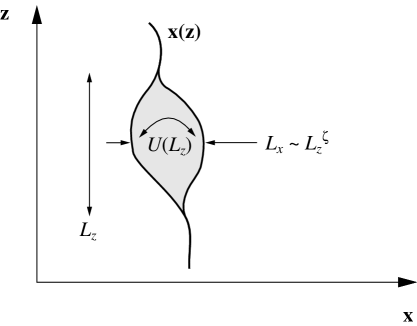
Figure 4: Illustration of two meta-stable configurations of the manifold (solid lines) that are separated by a barrier (shaded area). The characteristic length scales of the barrier are $L_{z}$ in longitudinal direction and $L_{x}$ in transverse direction. The height of the barrier is $U$.

A rigorous characterization of the statistics of barriers is very intricate. Therefore, a scaling picture [Villain 1984, Nattermann 1985b, Huse and Henley 1985, Ioffe and Vinokur 1987] has been put forward, where it is assumed that the statistics of barriers is essentially identical to the statistics of the free energy fluctuations. Therefore the barrier height should scale with the barrier length like

$$U(L_{z})\approx U_{\xi}\left(\frac{L_{z}}{L_{\xi}}\right)^{\psi},$$ (3.46)

where $U_{\xi}\equiv U(L_{\xi})\approx\varepsilon_{\parallel}\xi^{2}L_{\xi}^{D-2}$ is the typical height of the smallest possible barrier of the size of the Larkin length. The scaling exponent for the barrier height $\psi$ is assumed to coincide with the exponent $\theta$ from equation (3.31) that describes the free energy fluctuations:

$$\psi=\theta=2\zeta+D-2.$$ (3.47)

This exponent is related through equation (3.18) to the roughness exponent $\zeta$ of the manifold, which describes the scaling relation

$$L_{x}\approx\xi\left(\frac{L_{z}}{L_{\xi}}\right)^{\zeta}$$ (3.48)

between the lateral and transverse sizes of the barrier region.

The basic assumption $\psi=\theta$ has been confirmed by analytic arguments combined with numerical simulations [Mikheev et al. 1995, Drossel and Kardar 1995, Drossel 1996]. However, the statistics of barriers and free energy fluctuations have turned out to possibly be not strictly identical: $U(L_{z})$ and $\{\overline{[\Delta{\cal F}(L_{z})]^{2}}\}^{1/2}$ can differ by factors that are powers of $\ln L_{z}$ which do not modify the exponent relation (3.47).

It is clear that not all barriers of a given size $L_{z}$ have strictly the same height but that they are distributed according to a certain distribution ${\cal P}_{L_{z}}(U)$. The above scaling relations are valid for the ‘optimal’ (dynamically relevant) barrier height, which is the average barrier obtained from ${\cal P}_{L_{z}}(U)$ with an additional weighting factor for the density of barriers of the size considered [Vinokur et al. 1996]. In particular in low dimensions the dynamics of the manifold is not necessarily dominated by the average barrier height, but by the largest barriers. Therefore it is also of fundamental interest to characterize the distribution ${\cal P}_{L_{z}}(U)$ for large $U$.

For a string, i.e. $(D,N)=(1,1)$, [Vinokur et al. 1996] (?) found

$${\cal P}_{L_{z}}(U)\approx\frac{1}{U_{\xi}}\frac{L_{z}}{L_{\xi}}e^{-U/U_{\xi}}\exp[{-(L_{z}/L_{\xi})e^{-U/U_{\xi}}}]$$ (3.49)

from a combination of extreme value statistics [Gumbel 1958, Galambos 1978] and a coarse graining approach. Large barriers are exponentially rare since ${\cal P}_{L_{z}}(U)\sim\frac{1}{U_{\xi}}\frac{L_{z}}{L_{\xi}}e^{-U/U_{\xi}}$ for $U\to\infty$. [Gorokhov and Blatter 1999] (?) found that the free-energy distribution obeys a similar exponential decay at large negative values of the free energies ${\cal F}$. The free-energy distribution decays much faster at large positive ${\cal F}$ than at large negative ${\cal F}$, [Gorokhov and Blatter 1999], which one can expect because the manifold minimizes the free energy in equilibrium.

3.2 Transport properties

The glassy nature of systems does not manifest itself only in equilibrium properties but, maybe even more unambiguously, in its dynamic behaviour. The existence of many meta-stable states and the thermally activated nature of transitions between these states makes the dynamics of the glass extremely slow. We describe now the transport properties of manifolds in a stationary driven state, leaving aside interesting topics such as relaxational dynamics.

Vortices move dissipatively in the superconducting condensate. For small velocities the friction force is proportional to the velocity with a constant viscous drag coefficient $\eta_{0}$. For a single vortex line in a bulk superconductor [Bardeen and Stephen 1965]

$$\eta_{0}\approx\frac{\Phi_{0}H_{\rm c2}}{\rho_{\rm n}c^{2}},$$ (3.50)

where $\rho_{\rm n}$ is the normal state resistivity and $c$ the velocity of light. On large time scales inertial forces can be neglected in comparison to the friction force.

The equation of motion is then obtained from balancing the friction force (more precisely: the force density in a $D$-dimensional space; for brevity forces and force densities are not strictly distinguished) with the forces arising from the interaction with other vortices, the pinning force, the driving force ${\bf F}$ and a thermal noise ${{\zeta}}$,

$$\eta_{0}\dot{\bf x}=-\frac{\delta{\cal H}[{\bf x}]}{\delta{\bf x}}+{\bf F}+{\mbox{\boldmath${{\zeta}}$}}.$$ (3.51)

The noise is taken as Gaussian distributed with zero average and variance

$$\langle\zeta_{\alpha}({\bf z},t)\zeta_{\beta}({\bf z}^{\prime},t^{\prime})\rangle=2\eta_{0}T\delta_{\alpha\beta}\delta({\bf z}-{\bf z}^{\prime})\delta(t-t^{\prime})$$ (3.52)

such that the equation of motion properly describes thermodynamic equilibrium according to the fluctuation-dissipation theorem in the absence of the driving force.

At finite temperatures the manifold will respond to the driving force with an average velocity ${\bf v}\equiv\overline{\langle\dot{\bf x}\rangle}$. For calculational simplicity it is advantageous to consider ${\bf v}$ as prescribed and to calculate the driving force ${\bf F}={\bf F}({\bf v})$ required to maintain this velocity. In the driven case we define the displacement ${\bf u}({\bf z})\equiv{\bf x}({\bf z})-{\bf X}-{\bf v}t$ such that $\langle{\bf u}\rangle=0$. This displacement follows the equation of motion

$$\eta_{0}\dot{\bf u} = -\frac{\delta{\cal H}[{\bf X}+{\bf v}t+{\bf u}]}{\delta{\bf u}}+{\bf F}-\eta_{0}{\bf v}+{\mbox{\boldmath${{\zeta}}$}}$$ (3.53)

$$= \varepsilon_{\parallel}{\mbox{\boldmath${{\nabla}}$}}_{\parallel}^{2}{\bf u}-{\mbox{\boldmath${{\nabla}}$}}_{\perp}V({\bf X}+{\bf v}t+{\bf u},{\bf z})+{\bf F}-\eta_{0}{\bf v}+{\mbox{\boldmath${{\zeta}}$}},$$

which serves as basis for the following analysis [recall that ${\mbox{\boldmath${{\nabla}}$}}_{\parallel}\equiv(\frac{\partial}{\partial z_{1}},\dots,\frac{\partial}{\partial z_{D}})$ and ${\mbox{\boldmath${{\nabla}}$}}_{\perp}\equiv(\frac{\partial}{\partial u_{1}},\dots,\frac{\partial}{\partial u_{N}})$].

3.2.1 Friction

In the absence of pinning, $V=0$, the manifold moves with constant velocity ${\bf v}={\bf F}/\eta_{0}$. Pinning tends to slow down the motion of the system, because the manifold has to overcome barriers and it loses more time by sliding uphill than it wins by sliding downhill. Thus, to establish a certain velocity ${\bf v}$ in the presence of pinning, one has to apply a force ${\bf F}({\bf v})$ which is larger than in the absence of pinning. In general, the velocity-force characteristic will be non-linear but one can define an effective zero-velocity friction coefficient by

$$\eta_{\alpha\beta}\equiv\left.\frac{dF_{\alpha}({\bf v})}{dv_{\beta}}\right|_{\bf v=0}.$$ (3.54)

We now show that this ‘renormalized’ friction coefficient can diverge due to the presence of disorder, which is another signature of glassiness.

The divergence of the effective friction coefficient is examined by treating disorder perturbatively. We make use of the linear response function of the disorder-free system

$$G_{\alpha\beta}({\bf z},t) \equiv \frac{\delta\langle u_{\alpha}({\bf z},t)\rangle}{\delta F_{\beta}({\bf 0},0)}=\frac{1}{\eta_{0}}\left(\frac{\eta_{0}}{4\pi\varepsilon_{\parallel}t}\right)^{D/2}e^{-\eta_{0}z^{2}/2\varepsilon_{\parallel}t}\ \Theta(t)\delta_{\alpha\beta},$$ (3.55)

which describes the reaction of the displacement to a locally perturbating force.

By iterating the equation of motion (3.53) up to $O(V^{2})$, the condition $\overline{{\bf u}}=0$ yields the velocity-force characteristic and the effective friction coefficient

$$\eta_{\alpha\beta} = \eta_{0}\delta_{\alpha\beta}+\int dt\ t\ G_{\gamma\delta}({\bf z}=0,t)\partial_{\alpha}\partial_{\beta}\partial_{\gamma}\partial_{\delta}\Delta({\bf 0}).$$ (3.56)

Inspecting the large-time behaviour of the response function (3.55) for ${\bf z}={\bf 0}$, this coefficient diverges in $D\leq 4$ as long as $\partial_{\alpha}\partial_{\beta}\partial_{\gamma}\partial_{\delta}\Delta({\bf 0})\neq 0$ for certain indices. The divergence of $\eta_{\alpha\beta}$ resembles that of the susceptibility fluctuations (3.38): both couple to the fourth derivative of $\Delta({\bf u})$. This divergence actually does not mean that a stationary state with non-vanishing velocity could be established only by an infinite driving force; it means that at small velocities ${\bf v}({\bf F})$ is no longer linear (Ohmic) but sub-linear.

The qualitative change of the transport characteristic in $D\leq 4$ is consistent with roughening as a qualitative structural change. This consistency is not just a fortunate coincidence. One can actually show the relation between dynamic and static features using a fluctuation-dissipation relation between the correlation and response function of the free system [Scheidl and Vinokur 1998b]. Nevertheless, the toy model studied in Sec 3.1.3 has a strictly linear transport characteristic (the same as in the absence of disorder) despite its roughness. The transport characteristic is not at all affected by random bonds coupling to the displacement as in equation (3.32) because the translation symmetry ${\bf u}\to{\bf u}+{\bf x}_{0}$ is not broken. Thus the qualitative sensitivity of the transport characteristic to the nature of disorder suggests its use as a supplementary indicator for glassiness.

If the dynamics of the system is glassy, the transport characteristic shows several characteristic features, cf. figure 5. For small driving forces it is important to distinguish between the cases of zero and finite temperature. At $T=0$ the driving force has to exceed a threshold value $F_{c}$ to set the manifold in motion with a finite average velocity, since the driving force has to overcome the average pinning force. (Strictly speaking, this is true only in the absence of quantum fluctuations, which can lead to quantum creep at $T=0$ and $F\leq F_{c}$, see [Blatter et al. 1994] (?) and references therein.) This threshold phenomenon is called depinning. For $T>0$ a finite velocity is found even for $|{\bf F}|<F_{c}$ due to thermal activation, and the transport characteristic will be sub-linear (creep regime). At large driving forces $|{\bf F}|\gg F_{c}$ the effect of pinning diminishes and the free differential mobility is reached asymptotically, $dF_{\alpha}({\bf v})/dv_{\beta}\to\delta_{\alpha\beta}\eta_{0}$. This latter regime is called the flow regime.

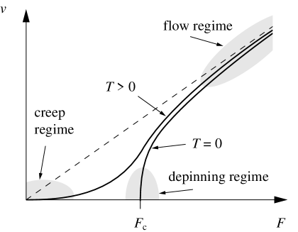
Figure 5: Illustration of the dynamic regimes (shaded areas) in the transport characteristic $v(F)$ of a manifold driven in disorder. In the absence of disorder the characteristic is linear (dashed line). In the presence of disorder it is non-linear (solid lines). At $T=0$ the manifold depins as a critical force $F_{c}$. At $T>0$ thermally activated creep occurs already for $F\ll F_{c}$. For $F\gg F_{c}$ the manifold flows essentially as in the absence of disorder.

The divergence of $\eta_{\alpha\beta}$ implies the break-down of perturbation theory for a calculation of the transport characteristic. Although it is difficult to calculate the global form of the characteristic, it is possible to achieve an analytic description for small and large velocity.

3.2.2 Depinning

The value of the critical force $F_{c}$ where motion sets in at $T=0$ can be estimated as follows: On length scales below the Larkin length $L_{\xi}$ the manifold performs only displacements smaller than $\xi$, such that the dependence of the pinning force on the displacement can be neglected. In such a volume the local pinning forces add up to ${\bf f}_{\xi}=\int_{|z|<L_{\xi}}d^{D}z\ [-{\mbox{\boldmath${{\nabla}}$}}_{\perp}V({\bf X},{\bf z})]$. The forces from different volumes are essentially uncorrelated. Thus depinning, where the driving force is balanced by pinning force, is found at [Feigel man 1983, Bruinsma and Aeppli 1984]

$$F_{c}\simeq L_{\xi}^{-D}\ {(\overline{{\bf f}_{\xi}^{2}})}^{1/2}\simeq(\Delta^{(2)})^{1/2}L_{\xi}^{-D/2}\simeq\varepsilon_{\parallel}\xi L_{\xi}^{-2}\sim(\Delta^{(2)})^{2/\epsilon},$$ (3.57)

where again $\epsilon\equiv 4-D$ and the pinning force variance $\Delta^{(2)}$ was given in equation (3.14). For fixed but weak strength of $\Delta^{(2)}$ the critical force $F_{c}$ vanishes as $D\nearrow 4$ and it is zero for $D>4$.

Thus for weak disorder (de)pinning occurs in $D\leq 4$ dimensions only, to which we restrict our analysis. The velocity is expected to increase continuously when the driving force exceeds the threshold value. This observation was made originally by [Middleton 1992a] (?) in the context of charge-density waves. Thus it should be possible to consider depinning as a continuous transition, at which the manifold exhibits critical fluctuations [Nattermann et al. 1992]. The depinning transition was studied theoretically for directed manifolds [Nattermann et al. 1992, Narayan and Fisher 1993, Ertaş and Kardar 1996, Leschhorn et al. 1997] and for the closely related charge-density waves [Fisher 1985b, Narayan and Fisher 1992a] within a renormalization group approach. [Kardar 1998] (?) and [Fisher 1998] (?) review depinning and its relevance in a much wider variety of phenomena.

The phenomenology of the transition is described qualitatively by the following scenario: as long as the manifold is pinned, it will be in a rough state because of competition between elastic forces, pinning forces, and the driving force. In the absence of the driving force, the roughness is described by the exponent $\zeta_{\rm rm}=\zeta_{\rm rm}(0)$ of manifolds in a random potential at equilibrium, which was described in equation (3.23). A driving force polarizes the state of the manifold and turns the situation into a non-equilibrium one, where the exponent is modified to $\zeta_{\rm rm}(F)$. Preliminary numerical simulations [Leaf et al. 1999] indicate that for forces $|{\bf F}|\leq F_{c}$ below the depinning transition, $\zeta_{\rm rm}(F)$ continuously increases with the driving force, until it reaches the value $\zeta_{\rm rm}(F_{c})=\zeta_{\rm rfi}$ of manifolds in a random force field at equilibrium, which was described in equation (3.27). This means that the effective force acting on the manifold has qualitatively changed its character. Above depinning, where the manifold moves with a finite velocity, the force acts on large scales like an effective thermal noise (although we consider the situation at $T=0$, without thermal noise $\zeta$ in the equation of motion). Accordingly, the manifold will be flat on large scales, as long as $D>2$.

For small velocities, the saturation of the displacement correlation function occurs on a large length scale $\ell_{z}$, which acts as a dynamical correlation length that diverges at the transition as [Middleton 1992a, Nattermann et al. 1992, Narayan and Fisher 1993]

$$\ell_{z}\sim(F-F_{c})^{-\nu}$$ (3.58)

with a certain exponent $\nu$. For this zero-temperature non-equilibrium transition, the force acts as a control parameter that plays the role of temperature in a usual finite-temperature equilibrium transition. Associated with the longitudinal scale $\ell_{z}$ there is a transverse scale

$$\ell_{x}\sim\ell_{z}^{\zeta}$$ (3.59)

with $\zeta$ being the roughness exponent at depinning. As the transition is approached from above, $F\searrow F_{c}$, there is also a diverging time scale $t_{v}$, the correlation time of the pinning force acting on the manifold,

$$t_{v}\approx\frac{\ell_{x}}{v}.$$ (3.60)

The dynamical exponent $z$ then can be defined from the scaling relation between $\ell_{z}$ and $t_{v}$,

$$t_{v}\sim\ell_{z}^{z}.$$ (3.61)

A further scaling relation describes the continuous onset of motion,

$$v\sim(F-F_{c})^{\beta}.$$ (3.62)

From a balance of the elastic and driving force in the equation of motion (making use of the non-renormalization of the elastic constant) one derives [Nattermann et al. 1992, Narayan and Fisher 1993]

$$\nu=\frac{1}{2-\zeta}.$$ (3.63)

The consistency of equations (3.60), (3.61) and (3.62) requires the scaling relation

$$\beta=(z-\zeta)\nu.$$ (3.64)

In the general case with more than one displacement component (for $N>1$), the velocity selects one particular direction out of the $N$-dimensional space and we may choose the coordinates such that ${\bf v}=v\delta_{\alpha,1}$. Due to this selection of a direction by velocity one has to expect the displacement correlations to be uniaxially anisotropic. We subsequently distinguish $W_{\alpha}({\bf z},t)=\overline{\langle[u_{\alpha}({\bf z},t)-u_{\alpha}({\bf 0},0)]^{2}\rangle}$, where $\alpha=1$ for the parallel component and $\alpha=2,\dots,N$ for the perpendicular component. The anisotropy is not a minor quantitative effect, it concerns the scaling exponents as shown by [Ertaş and Kardar 1996] (?). The anisotropic scaling laws for the displacement components are

$$W_{\alpha}({\bf z},t) = |{\bf z}|^{2\zeta_{\alpha}}g_{\alpha}(t/|{\bf z}|^{z_{\alpha}}),$$ (3.65)

with $g_{\alpha}(0)$ finite and $g_{\alpha}(y)\sim y^{2\zeta_{\alpha}/z_{\alpha}}$ for large arguments $y$. The above scaling relations (3.63) and (3.64) then hold with the identification

$$\zeta\equiv\zeta_{1},\quad z\equiv z_{1}.$$ (3.66)

The values of the exponents which can be calculated analytically within a renormalization group approach, using an expansion in small $\epsilon=4-D$ [Nattermann et al. 1992, Ertaş and Kardar 1996] are:

$$\zeta_{1} = \frac{\epsilon}{3}$$ (3.67a)

$$z_{1} = 2-\frac{2\epsilon}{9}+O(\epsilon^{2})$$ (3.67b)

$$\zeta_{\alpha} = \zeta_{1}-\frac{D}{2}=-2+\frac{5\epsilon}{6}$$ (3.67c)

$$z_{\alpha} = z_{1}+\frac{1}{\nu}=4-\frac{5\epsilon}{9}+O(\epsilon^{2})$$ (3.67d)

and all directions $\alpha\geq 2$ scale identically. Equation (3.67a) means that the manifold in a random potential at depinning has the roughness of a manifold in random force field in equilibrium, cf. equation (3.27). [Narayan and Fisher 1993] (?) proved that equation (3.67a) is correct to all orders in $\epsilon$.

For the depinning of periodic media such as charge-density waves the same scenario holds as for directed manifolds. However, they belong to a different universality class with different values of the exponents [Middleton 1992a, Narayan and Fisher 1992b, Narayan and Fisher 1992a].

So far, we have discussed depinning as a phenomenon at $T=0$. The effect of finite temperature is that potential barriers can be overcome by thermal activation. Therefore a finite velocity is expected for every finite driving force. Fixing the force at the $T=0$ threshold value $F=F_{c}$, velocity increases with temperature according to a power law

$$v\sim T^{\beta/\tau}.$$ (3.68)

The exponent $\tau$ depends on the type of the pinning potential in a non-universal way [Fisher 1985b, Middleton 1992b]. For the ‘ratcheted kick model’ [Middleton 1992b] (?) argued for $\tau=2$ in $D=2,3$. The actual value of $\tau$ is still controversial and subject to investigations [Nowak and Usadel 1998, Roters et al. 1999].

3.2.3 Creep

Below the depinning threshold, for $|{\bf F}|\leq F_{c}$, the dynamics of the manifold is in the creep regime, where motion is possible only through thermal activation. At $|{\bf F}|=F_{c}$, barriers of all sizes are equally relevant and it is precisely for this reason that depinning appears as a critical phenomenon. Below depinning, barriers of a typical size are prevalent and dominate the thermally activated dynamics. In the presence of a driving force the manifold experiences an effective potential $V_{\rm eff}({\bf x},{\bf z})\equiv V({\bf x},{\bf z})-{\bf x}\cdot{\bf F}$. For weak forces the manifold still has meta-stable states in this effective potential, which are separated by barriers that also depend on the driving force.

We now focus on the creep regime of very small forces $|{\bf F}|\ll F_{c}$, where the barriers are nearly identical to those in equilibrium and where a scaling picture for the typical, dynamically relevant barrier has been developed. The starting point of this picture is the assumption that barriers of a length $L_{z}$ and free energy fluctuations of a system of size $L_{z}$ have identical scaling as described in equation (3.46). The typical lengths $L_{z}$ and $L_{x}\sim L_{z}^{\zeta}$ are related by equation (3.48). When the manifold overcomes such a barrier, it gains an energy

$$E_{F}\approx FL_{x}L_{z}^{D}\approx F\xi L_{\xi}^{D}\left(\frac{L_{z}}{L_{\xi}}\right)^{D+\zeta}$$ (3.69)

in the field of the driving force. Therefore, in the effective potential $V_{\rm eff}$ only those barriers are still effective for which $U\lesssim E_{F}$. From $U(L_{F})=E_{F}$ follows [Ioffe and Vinokur 1987, Nattermann 1987, Feigelman and Vinokur 1988, Feigel’man et al. 1989, Nattermann 1990] the size of the largest effective barrier

$$L_{F} \equiv L_{z}(F)\approx L_{\xi}\left(\frac{F}{F_{\xi}}\right)^{-1/(D+\zeta-\theta)}\sim F^{-1/(D+\zeta-\theta)}$$ (3.70a)

$$U(F) \equiv U(L_{F})\approx U_{\xi}\left(\frac{F}{F_{\xi}}\right)^{-\mu}\sim F^{-\mu}$$ (3.70b)

with the creep exponent

$$\mu\equiv\frac{\theta}{D+\zeta-\theta}=\frac{2\zeta+D-2}{2-\zeta}.$$ (3.71)

We have used the abbreviation $F_{\xi}\equiv U_{\xi}L_{\xi}^{-D}\xi^{-1}$ and the identity (3.18). The effectiveness of barriers of a given size $L_{z}$ is illustrated in figure 6. If one denotes by $F_{\rm B}(L_{z})\equiv U(L_{z})/(L_{x}L_{z}^{D})\sim L_{z}^{\zeta-2}$ the threshold force density which is required to overcome barriers of size $L_{z}$, the size of the largest effective barrier is determined alternatively by $F=F_{\rm B}(L_{F})$.

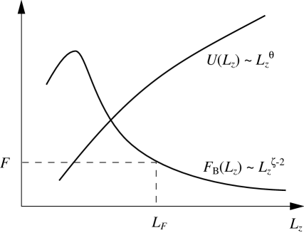
Figure 6: The height of barriers scales like $U\sim L_{z}^{\theta}$ with the barrier size $L_{z}$ (in general, $\theta>0$ at a zero-temperature fixed point). The effective pinning force of these barriers scales like $F_{B}\sim L_{z}^{\zeta-2}$ (the manifold model is valid only as long as $\zeta<1$). In the presence of a driving force $F$ only barriers of a size $L_{z}<L_{F}$ are still effective.

Since the time $t$ to overcome a barrier by thermal activation increases exponentially with the height $U$,

$$t(U)\sim e^{U/T},$$ (3.72)

it is the largest effective barrier that dominates the dynamics and determines the creep velocity

$$v(F)\sim(F/\eta_{0})e^{-U(F)/T}\sim(F/\eta_{0})e^{-(U_{\xi}/T)(F/F_{\xi})^{-\mu}}.$$ (3.73)

The pre-exponential factor has been inserted by hand for dimensional reasons and to match the flow regime. However, in the creep regime this factor may be of more complicated form (corresponding to a logarithmic contribution to $U(F)$) which is not captured by this scaling argument.

From equation (3.73) we see that the dynamic response will be exponentially small below depinning, since a disorder-dominated roughness with exponent $\zeta>\zeta_{\rm th}=(2-D)/2$ implies $\mu>0$. The characteristic dynamic exponent $\mu$ depends only on the dimension and the static roughness exponent of the system.

In order to provide a deeper understanding of these scaling relations several authors [Radzihovsky 1998, Balents et al. 1998b, Chauve et al. 1998] have recently developed a renormalization group analysis for the whole range of velocities. For $T=0$ their approach correctly reproduces the properties of the depinning transition and for $T>0$ they obtain a more precise characteristic $v(F)$, which confirms the exponential dependence of the characteristic (3.73) to leading order for small forces but contains also subleading orders.

Experimental observations on magnetic domain walls, charge-density waves, and VLL are widely consistent with this scaling picture of barriers. The most explicit measurement of the roughness and creep exponent examining magnetic domain wall creep [Lemerle et al. 1998] was made only recently and is in good agreement with the theoretical results.

3.2.4 Flow

The flow regime at large driving force $|{\bf F}|\gg F_{c}$ does not usually receive much attention since it is considered trivial and is expected to be captured within perturbation theory. However, recently the flow regime has attracted some attention for driven VLL, where it turned out to be quite non-trivial and inaccessible to a perturbative analysis (see section 7) due to an intricate interplay of pinning forces and driving force. Therefore we will briefly sketch this regime also for the manifolds.

Let us consider again zero temperature. There the displacements are expected to be very small for large driving forces: the manifold can respond to the pinning force only with certain (scale-dependent) relaxation times and the pinning force changes rapidly in time for large $F$. Therefore the effect of pinning effectively gets averaged out for $F\to\infty$.

Since the disorder induced displacements are small at large $F$, one may again perform a perturbative analysis as a first step. According to the equation of motion (3.53) the effect of disorder is given to lowest order by a pinning force

$${\bf F}^{\rm pin}({\bf z},t)=-{\mbox{\boldmath${{\nabla}}$}}_{\perp}V({\bf X}+{\bf v}t,{\bf z}),$$ (3.74)

which shakes the manifold as it moves over the pinning potential. Its average is zero and its variance is

$$\overline{F^{\rm pin}_{\alpha}({\bf z},t)F^{\rm pin}_{\beta}({\bf 0},0)}=-\partial_{\alpha}\partial_{\beta}\Delta({\bf v}t)\delta({\bf z}).$$ (3.75)

For qualitative purposes this shaking force might be compared to an effective thermal noise. Because the velocity selects a particular space direction this noise in no longer isotropic. Effective shaking temperatures (which were introduced by [Koshelev and Vinokur 1994] (?) for vortex lattices) for the directions parallel and perpendicular to ${\bf v}\equiv(v,{\bf 0})$ can be identified from

$$T^{\rm sh}_{\alpha} = \frac{1}{2\eta_{0}}\int dtd^{D}z\ \overline{F^{\rm pin}_{\alpha}({\bf z},t)F^{\rm pin}_{\alpha}({\bf 0},0)}$$ (3.76a)

$$T^{\rm sh}_{1} = 0,$$ (3.76b)

$$T^{\rm sh}_{\alpha} \sim \frac{\Delta_{0}}{2\eta_{0}v\xi^{D+1}},\quad(\alpha\geq 2).$$ (3.76c)

These shaking temperatures are to be added to the physical temperature to give the total effective temperature, which is finite. Thus, for $D>2$ the manifold should be flat with exponent $\zeta=\zeta_{\rm th}=\frac{2-D}{2}$ as in the absence of disorder. This flatness is expected to persist at any finite velocity, i.e., for all forces above $F_{c}$. However, it is interesting to observe that in the flow regime the manifold has a larger width in the direction perpendicular to ${\bf v}$ since $T^{\rm sh}_{\alpha}>T^{\rm sh}_{1}$ (with $\alpha\geq 2$). On the contrary, at depinning the manifold has a larger width in the direction parallel to ${\bf v}$ since $\zeta_{\alpha}<\zeta_{1}$, see equation (LABEL:dep.exp). This means that at a certain velocity the manifold has to reverse the aspect ratio of its widths. Apart from this interesting observation, perturbation theory gives no hints of qualitative changes of the state with changing velocity such as dynamic phase transitions. However, such transitions exist in periodic structures such as VLL (section 7).

3.3 Summary

In this chapter we have reviewed various properties of manifolds in order as to identify a glassy state of the system. Of course, disorder always quantitatively modifies the state on small length scales. Some large-scale properties of the system can be modified qualitatively by disorder and are hence suitable for the characterization of glassiness:

• Disorder reduces the positional order and it increases the roughness. Typically, $\zeta>\zeta_{\rm th}$ but such an increase is also possible for $\zeta=\zeta_{\rm th}$ if $W$ is increased only by logarithmic factors.

• Disorder leads to large sample-to-sample fluctuations, which can be described by susceptibilities.

• In a renormalization-group description of the large-scale physics, there is a disorder-dominated fixed point. Typically, this is a zero-temperature fixed point. In low dimensions ($D\leq 2$), this may also be a finite-temperature fixed point.

• Disorder induces thermally activated sub-linear response to a driving force.

We consider all these features as generic to identify the glassy nature of a system. The insufficiency of individual features can be shown by examples: An increased roughness alone is not significant as emphasized by [Hwa and Fisher 1994b] (?) using the bond-disorder model, which has no broken translation symmetry. Sub-linear response is a signature of broken translation symmetry but can also be achieved by ‘ordered’ potentials. Similarly, a zero-temperature fixed point can, in general, represent a low-temperature ordered phase which is not necessarily a glass. The sine-Gordon model provides an example for the last two statements.

4 Superconducting film in a parallel field

In treating a many-vortex system we begin with the technically most simple problem of a superconducting film in a magnetic field parallel to the film plane. The mean-field phase diagram of this problem was considered by [Abrikosov 1964] (?), who found for $H_{\rm c1}<H<H_{\rm c2}$ a solution with an equidistant vortex lattice of spacing $a$. Here $H_{\rm c1}=\frac{2}{\pi}\frac{\Phi_{0}}{s^{2}}\ln\frac{s}{\xi}$ and $H_{\rm c2}=\frac{\sqrt{3}}{\pi}\frac{\Phi_{0}}{\xi s}$, where $s$ is the thickness of the film and we assume $\lambda>s/\pi\gtrsim\xi$ (see [Sonin 1992] (?) for films described by the Lawrence-Doniach model). Such a geometry can be realized experimentally and the vortex physics was observed recently on mesoscopic scales [Bolle et al. 1999].

In such a planar geometry vortices are not strictly confined within the film. In principle they may leave and enter the film on a side. However, such events, as well as a crossing of vortex lines within the film, always cost energy. In our theoretical analysis we will neglect such events. Then, by construction, vortex lines leave the superconducting plane only at its boundary, the vortex lattice does not exhibit topological defects like dislocations and, hence, it cannot melt unless we reach $T_{\rm c}$. Thermal fluctuations lead therefore to a quasi-long-range ordered lattice as in other 2D crystals [Mermin and Wagner 1966] which persists roughly up to the mean-field transition temperature $T_{\rm c0}$. In the following we consider the influence of frozen-in disorder on this system. It turns out that the problem can be mapped onto a magnetic model, the $XY$ model in a random field, for which many results are known. In addition to the phase with quasi-long-range order there is a low-temperature glassy phase, which is the result of the balance between thermal and disorder fluctuations (in this sense, the situation is different from that for bulk materials, where thermal fluctuations have a much weaker effect on the formation of the glassy state). Drift of the vortices due to an external current (perpendicular to the film plane) leads in the glassy phase to a vanishing linear resistivity.

4.1 Mapping on the $XY$ model in a random field

The mapping of this model onto a two-dimensional $XY$ model in a random field was first considered by [Fisher 1989] (?) in his seminal paper on vortex glasses. Here we will follow a slightly different derivation.

To formulate the model, we assume that the superconducting film is in the $(x,z)$ plane and that the vortex lines are directed along the $z$ axis with an average line spacing $a$. The position of the $n$th vortex line is denoted by $x_{n}(z)=X_{n}+u_{n}(z)$, where $X_{n}=na$ and $u_{n}(z)\equiv u(X_{n},z)$ are the rest position and the displacement, respectively. The Hamiltonian can then be written in the form ${\cal H}={\cal H}_{\rm el}+{\cal H}_{\rm pin}$, where

$${\cal H}_{\rm el} = \int d^{2}r\left\{\frac{c_{11}}{2}(\partial_{x}u)^{2}+\frac{c_{44}}{2}(\partial_{z}u)^{2}\right\},$$ (4.1a)

$${\cal H}_{\rm pin} = \int d^{2}r\ \rho_{u}({\bf r})V({\bf r}).$$ (4.1b)

Here ${\bf r}\equiv(x,z)$, $c_{11}$ and $c_{44}$ are the compression and tilt elastic constant, $\rho_{u}({\bf r})$ the vortex line density and $V({\bf r})$ the random pinning potential. For the latter we assume for simplicity

$$\overline{V({\bf r})} = 0,$$ (4.2a)

$$\overline{V({\bf r})V({\bf r}^{\prime})} = \Delta(x-x^{\prime})\delta(z-z^{\prime})$$ (4.2b)

and, as before, $\Delta(x)\approx\Delta_{0}/(\sqrt{2\pi}\xi)e^{-x^{2}/2\xi^{2}}$, but $\Delta_{0}\approx n_{\rm i}^{(2)}f_{\rm pin}^{2}\xi^{3}s$, where $n_{\rm i}^{(2)}$ and $f_{\rm pin}$ denote the impurity density per unit area and the individual force of a single impurity on the vortex line, respectively [Blatter et al. 1994].

In general, the elastic Hamiltonian will be non-local, reflecting the dispersion of the elastic constants for wave vectors $|{\bf k}|>\lambda^{-1}$. Since we, however, are interested in the disordered case, which is dominated by large scale fluctuations, we ignore this fact here. This approximation is justified in particular for weak disorder, a case in which all relevant length scales are much larger than $\lambda$. Thermal and disorder fluctuations will considerably renormalize $c_{11}$ and $c_{44}$ with respect to their mean-field values.

If one starts with isolated vortex lines of displacements $u_{n}$ which have a stiffness constant $\varepsilon_{\parallel}$ and a mutual short-ranged interaction energy $U(a+u_{n+1}-u_{n})$, then

$$c_{11}=aU^{\prime\prime}(a),\quad c_{44}=\varepsilon_{\parallel}/a.$$ (4.3)

On scales $a\gg\lambda$ mean-field theory yields $U(a)=U_{\rm MF}(a)\sim e^{-a/\lambda}$.

Thermal fluctuations on scales $|\Delta x|\leq a$ lead to a steric repulsion [Pokrovsky and Talapov 1979] between the vortex lines, which reads for $\lambda\to 0$

$$U_{\rm th}(a)=\frac{T^{2}}{\varepsilon_{\parallel}a^{2}}\frac{\pi^{2}}{6},$$ (4.4)

such that $(c_{11}c_{44})^{1/2}/T=\pi/a^{2}$ becomes independent of temperature. As we will see below [cf. (4.25)], this relation is exactly the condition for the glass transition temperature $T_{\rm g}=(c_{11}c_{44})^{1/2}a^{2}/\pi$. In other words, the relation (4.4) maps the system at all temperatures to the glass transition temperature $T_{\rm g}$. However, in deriving (4.4) only a hard-core repulsive interaction between vortex lines was assumed (indeed, [Pokrovsky and Talapov 1979] (?) mapped their problem onto non-interacting fermions). If we include an additional interaction energy of the order of $U_{c}$ per contact point of two fluctuating vortex lines, we get

$$c_{11}^{\rm th}(a)\approx\frac{T^{2}}{\varepsilon_{\parallel}a^{3}}\left({\pi^{2}}+\frac{U_{c}}{T}\right).$$ (4.5)

This leads to $T_{\rm g}\equiv(c_{11}c_{44})^{1/2}a^{2}/\pi=T(1+U_{c}/\pi^{2}T)^{1/2}$, which corresponds to $T\gtrless T_{\rm g}$ for $U_{c}\lessgtr 0$.

Disorder leads also to a steric repulsion [Kardar and Nelson 1985, Nattermann and Lipowsky 1988] of the form (we drop here coefficients of order unity because they cannot be determined very accurately)

$$U_{\rm pin}(a)\approx\frac{\Delta_{0}}{T+T_{\Delta}}\frac{1}{a},$$ (4.6)

where $T_{\Delta}\approx(\varepsilon_{\parallel}\xi\Delta_{0})^{1/3}$ [Nattermann and Renz 1988]. This gives

$$\frac{T_{\rm g}}{T}=\frac{a^{2}}{\pi T}\sqrt{c_{11}c_{44}}\approx\frac{T_{\Delta}}{T}\left(\frac{a}{\xi}\frac{T_{\Delta}}{T+T_{\Delta}}\right)^{1/2}\approx\sqrt{\frac{a}{a_{c}}}.$$ (4.7)

The vortex-line distance

$$a_{c}\approx\xi\frac{T^{2}(T+T_{\Delta})}{T_{\Delta}^{3}}$$ (4.8)

denotes a cross-over length scale from a thermal steric repulsion (for $a\lesssim a_{c}$) to a disorder dominated steric repulsion (for $a\gtrsim a_{c}$). The formulas for $U_{\rm pin}$ and $a_{c}$ are not exact but represent crude interpolation formulas between the limiting cases $T\ll T_{\Delta}$ and $T\gg T_{\Delta}$.

Finally, a contact interaction can also be included in $U_{\rm pin}(a)$ such that

$$c_{11}^{\rm pin}(a)\approx\frac{T^{2}}{\varepsilon_{\parallel}a^{2}a_{c}}\left(1+\frac{U_{c}}{T}\sqrt{\frac{a_{c}}{a}}\right).$$ (4.9)

Here we have written $c_{11}^{\rm pin}(a)$ in a form similar to $c_{11}^{\rm th}(a)$. Comparing these two quantities, it is easy to see that $c_{11}^{\rm pin}(a)>c_{11}^{\rm th}(a)$ in the region $a>a_{c}$, and hence we are below $T_{\rm g}$ (provided $U_{c}>0$).

One should, however, take into account that all these expressions were derived under the assumption that the bare interaction between vortex lines is short ranged, i.e., for the case $\lambda\ll a$. In the opposite case the calculation is more involved and will not be considered here further.

Next we consider the pinning energy (4.1b). Using the Poisson-summation formula, we may rewrite the density $\rho_{u}({\bf r})$ as ([Nattermann 1990, Nattermann et al. 1991]; see also appendix A)

$$\rho_{u}({\bf r}) = \sum_{n=-\infty}^{\infty}\delta(x-X_{n}-u_{n}(z))$$ (4.10)

$$= \sum_{n=-\infty}^{\infty}\int_{-\infty}^{\infty}dX\ \delta(X-X_{n})\delta(x-X-u_{n}(z))$$

$$= \frac{1}{a}\sum_{m=-\infty}^{\infty}\int_{-\infty}^{\infty}dX\ e^{iQ_{m}X}\delta(x-X-u(X,z))$$

$$= \frac{1}{a}\int_{-\infty}^{\infty}dX\ (1+2\sum_{m\geq 1}\cos(Q_{m}X))\delta(x-X-u(X,z))$$

$$\approx \frac{1}{a}\bigg{\{}1-\partial_{x}u({\bf r})+2\sum_{m\geq 1}\cos(Q_{m}[x-u({\bf r})])\bigg{\}}.$$

$Q_{m}\equiv 2\pi m/a$ is a reciprocal lattice vectors of the 2D line array. The pinning energy (4.1b) can hence be written as

$${\cal H}_{\rm pin} = \int d^{2}r\ \bigg{\{}-\frac{1}{2\pi}\partial_{x}\varphi({\bf r})V({\bf r})$$ (4.11a)

$$+\sum_{m\geq 1}[h_{1m}({\bf r})\cos(m\varphi({\bf r}))+h_{2m}({\bf r})\sin(m\varphi({\bf r}))]\bigg{\}},$$

$$h_{1m}({\bf r}) \equiv \frac{2}{a}V({\bf r})\cos(Q_{m}x),\quad\quad h_{2m}({\bf r})\equiv\frac{2}{a}V({\bf r})\sin(Q_{m}x),$$ (4.11b)

where we introduced the phase field $\varphi\equiv 2\pi u/a$ [which should not be confused with the phase $\phi$ of the superconducting order parameter; see equation (4.38) below]. The disorder fields $h_{\alpha m}$ ($\alpha,\beta=1,2$) are Gaussian distributed with

$$\overline{h_{\alpha m}({\bf r})} = 0,$$ (4.12a)

$$\overline{h_{\alpha m}({\bf r})h_{\beta n}({\bf r}^{\prime})} \approx 2\frac{\Delta_{0}}{a^{2}}f_{\alpha m,\beta n}(Q_{m}x,Q_{n}x^{\prime})\delta_{\xi}({\bf r}-{\bf r}^{\prime}).$$ (4.12b)

On scales $\Delta x\gg a$, $f_{\alpha m,\beta n}(Q_{m}x,Q_{n}x^{\prime})\approx\delta_{\alpha\beta}\delta_{mn}$ since the rapidly fluctuating contributions with $m\neq n$ or $\alpha\neq\beta$ average to zero. On these scales, ${\cal H}_{\rm pin}$ can also be written in the form

$${\cal H}_{\rm pin}\approx\int d^{2}r\ \bigg{\{}-\frac{1}{2\pi}\partial_{x}\varphi({\bf r})V({\bf r})+\sum_{m\geq 1}\frac{2}{a}\Delta_{0}^{1/2}\cos(m\varphi({\bf r})-\alpha_{m}({\bf r}))\bigg{\}}.$$ (4.13)

The random phases $\alpha_{m}({\bf r})$ obey

$$\overline{e^{i\alpha_{m}({\bf r})}} = 0,$$ (4.14a)

$$\overline{e^{i[\alpha_{m}({\bf r})-\alpha_{n}({\bf r}^{\prime})]}} = \delta_{mn}\delta_{\xi}({\bf r}-{\bf r}^{\prime}).$$ (4.14b)

The effect of fluctuations of individual vortex lines on scales $\Delta x\lesssim a$ was discussed briefly in the first part of this section. Since we study the film in a parallel field mainly because of the possibility of obtaining explicit results for the vortex-glass state in a case which we understand to a large extent (and not so much because of its experimental relevance), we will ignore collective fluctuation effects on small and intermediate scales but concentrate directly on the large-scale behaviour where typical phase fluctuations are of the order $2\pi$. On these scales terms with $m>1$ in (4.13) can be ignored since they are less relevant than that with $m=1$.

It is convenient to rewrite (4.1a) as

$${\cal H}_{\rm el} = \frac{J}{2}\int d^{2}r\ ({\mbox{\boldmath${{\nabla}}$}}\varphi)^{2}$$ (4.15)

by rescaling the $z$ coordinate and introducing the stiffness constant $J$ according to

$$\widetilde{z} \equiv \left(\frac{c_{11}}{c_{44}}\right)^{1/2}z,$$ (4.16a)

$$J \equiv \left(\frac{a}{2\pi}\right)^{2}\sqrt{{c_{11}}{c_{44}}}.$$ (4.16b)

This rescaling leaves ${\cal H}_{\rm pin}$ form-invariant apart from a multiplication with a factor $(c_{44}/c_{11})^{1/4}$. Thus ${\cal H}_{\rm el}+{\cal H}_{\rm pin}$ now equals the Hamiltonian of a random-field (RF) $XY$ model without vortices, which was considered in the context of magnetic models by a number of authors [Cardy and Ostlund 1982, Goldschmidt and Houghton 1982, Goldschmidt and Schaub 1984, Villain and Fernandez 1984].

After rescaling (4.16a), ${\cal H}_{\rm pin}$ can be written as

$${\cal H}_{\rm pin}=\int d^{2}r\ \left\{\widetilde{V}(\varphi({\bf r}),{\bf r})-{\mbox{\boldmath${{\mu}}$}}({\bf r})\cdot{\mbox{\boldmath${{\nabla}}$}}\varphi({\bf r})\right\}$$ (4.17)

with

$$\overline{{\mbox{\boldmath${{\mu}}$}}} = \overline{\widetilde{V}}=0,$$ (4.18a)

$$\overline{\mu_{i}({\bf r})\mu_{j}({\bf r}^{\prime})} = J^{2}\sigma\delta_{ij}\delta_{\xi}({\bf r}-{\bf r}^{\prime}),$$ (4.18b)

$$\overline{\widetilde{V}(\varphi,{\bf r})\widetilde{V}(\varphi^{\prime},{\bf r}^{\prime})} = h^{2}\cos(\varphi-\varphi^{\prime})\delta_{\xi}({\bf r}-{\bf r}^{\prime}),$$ (4.18c)

where we introduced the variances $\sigma$ and $h^{2}$. Their bare (unrenormalized) values are given by

$$h_{0}^{2} \equiv 2\frac{\Delta_{0}}{a^{2}}\left(\frac{c_{44}}{c_{11}}\right)^{1/2},$$ (4.19a)

$$\sigma_{0} \equiv \frac{h_{0}^{2}a^{2}}{8\pi J^{2}}.$$ (4.19b)

This relation between $\sigma$ and $h^{2}$ in (LABEL:def.h.sig) holds only for the unrenormalized quantities. However, under renormalization these quantities flow independently. Although (4.13) originally contained only a linear gradient term in the $x$ direction, we rewrote it here in an isotropic form, anticipating the generation of $\partial_{z}\varphi$ terms under the renormalization-group transformation.

Before we come to the renormalization-group calculation for the model (4.17), we will apply a Flory-type analysis to it. To be more general, we will present this analysis in $d$ dimensions. One complication with respect to the problem considered in section 3.1.1c is the fact that the correlator of the pinning Hamiltonian now contains the oscillatory term (4.18c). For weak disorder $ha\ll J$, a given configuration of the random phase $\alpha_{1}({\bf r})\equiv\alpha({\bf r})$ implies a certain ground-state configuration $\varphi_{0}({\bf r})=\varphi_{0}({\bf r},\{\alpha\})$ which depends on the value of the random phase everywhere in the system. Going through the different configurations of $\{\alpha\}$ will generate a distribution of ground state configurations $\{\varphi_{0}\}$ which we assume to be Gaussian distributed. Since $ha\ll J$, the correlation of the value of $\alpha({\bf r})$ and $\varphi_{0}({\bf r})$ at the same position ${\bf r}$ will be weak. In averaging over the distribution of $\alpha({\bf r})$ we can therefore neglect the local correlations between $\alpha({\bf r})$ and $\varphi_{0}({\bf r})$ in a first approximation. The typical energy gain from the pinning term then becomes

$$E_{\rm pin}\approx-\max\left\{J\sqrt{\sigma}L^{(d-2)/2}({\overline{\varphi^{2}}})^{1/2},hL^{d/2}e^{-{\overline{\varphi^{2}}}/2}\right\}.$$ (4.20)

Depending on the dimension $d$, the leading contribution to $E_{\rm pin}$ can be the random-tilt or the random-field contribution. The dependence of $\overline{\varphi^{2}}$ on the system size $L$ follows from equating the absolute value of $E_{\rm pin}$ to the averaged elastic energy

$$E_{\rm el}\approx JL^{d-2}\overline{\varphi^{2}}.$$ (4.21)

For $2<d<4$ one finds that the random-field contribution dominates in $E_{\rm pin}$, which results in

$$\overline{\varphi^{2}}\approx(4-d)\ln\frac{L}{L_{\xi}}-2\ln[\overline{\varphi^{2}}],$$ (4.22)

where we introduced the Larkin length $L_{\xi}\approx(J/h)^{2/(4-d)}$. Thus, the Flory argument gives at $T=0$ a logarithmic increase of $\overline{\varphi^{2}}$ in all $2<d<4$. We will see in section 6 that a renormalization-group calculation confirms essentially this result, apart from a (small) modification of the coefficient of the logarithm. For $d<2$ on the other hand, $E_{\rm pin}$ is dominated by the random-tilt contribution and the balance of $E_{\rm pin}$ and $E_{\rm el}$ at $T=0$ results in $\overline{\varphi^{2}}\approx\sigma L^{2-d}$ in agreement with renormalization-group calculations [Villain and Fernandez 1984]. We will show below that in $d=2$ dimensions $\sigma$ is renormalized to large values such that $E_{\rm pin}$ and $\overline{\varphi^{2}}$ are dominated by the random-tilt contribution.

4.2 Renormalization

After replication, we get from (4.17) and (LABEL:mu.corr)

$${\cal H}_{n}=\sum_{ab}\int d^{2}r\ \left\{\frac{1}{2}J(\delta^{ab}-\frac{J\sigma}{T}){\mbox{\boldmath${{\nabla}}$}}\varphi^{a}\cdot{\mbox{\boldmath${{\nabla}}$}}\varphi^{b}-\frac{h^{2}}{2T}\cos(\varphi^{a}-\varphi^{b})\right\}.$$ (4.23)

The RG flow equations of this model, first found by [Cardy and Ostlund 1982] (?), are then

$$\frac{dJ}{dl} = 0,$$ (4.24a)

$$\frac{d\sigma}{dl} = c_{1}\frac{h^{4}}{T^{2}J^{2}},$$ (4.24b)

$$\frac{dh}{dl} = \left(1-\frac{T}{T_{\rm g}}\right)h-c_{2}\frac{h^{3}}{T^{2}},$$ (4.24c)

with the glass transition temperature

$$T_{\rm g}=4\pi J.$$ (4.25)

The integration of (4.24c) yields

$$h^{2}(L)=h_{0}^{2}\left(\frac{L}{a}\right)^{2\tau_{\rm g}}\left\{1+\frac{h_{0}^{2}}{{h^{*}}^{2}}\left[\left(\frac{L}{a}\right)^{2\tau_{\rm g}}-1\right]\right\}^{-1}$$ (4.26)

with $l=\ln(L/a)$, the fixed-point value ${h^{*}}^{2}=T^{2}\tau_{\rm g}/c_{2}$ and the reduced temperature

$$\tau_{\rm g}\equiv 1-\frac{T}{T_{\rm g}}.$$ (4.27)

It can be shown quite generally that the flow of $\sigma$ does not feed back into that of $h$ [Hwa and Fisher 1994b]. The constants $c_{1}$ and $c_{2}$ are cut-off dependent, but their ratio

$$\frac{c_{1}}{c_{2}^{2}}=\frac{1}{4\pi}+O(\tau_{\rm g})$$ (4.28)

is universal. The whole calculation is valid only for $\tau_{\rm g}\ll 1$. Considering equivalent models, equivalent RG equations were found by [Goldschmidt and Houghton 1982] (?), [Rubinstein et al. 1983] (?), [Goldschmidt and Schaub 1984] (?), and [Paczuski and Kardar 1991] (?). The parameter flow is shown schematically in figure 7.

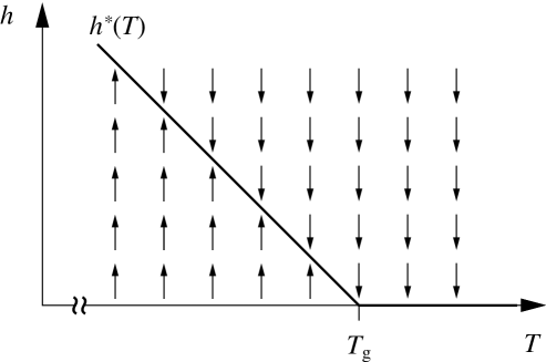
Figure 7: RG flow in the $(h,T)$-plane. The random-field amplitude $h$ flows to $h^{*}=0$ above the glass transition temperature ($T>T_{\rm g}$) whereas it flows to $h^{*}\propto(T_{\rm g}-T)$ below ($T<T_{\rm g}$).

The quantity $h^{2}$ approaches a fixed point ${h^{*}}^{2}\approx{T_{\rm g}^{2}\tau_{\rm g}}/{c_{2}}$. Integrating (4.24b) for $h\approx h^{*}$, we find on the length scale $L=ae^{l}$

$$\sigma(L)\approx 4\pi\tau_{\rm g}^{2}\ln(L/a).$$ (4.29)

If we go back to the renormalized but unrescaled quantities – these are the physical quantities we would measure in an experiment on this scale – we obtain for the effective parameters on scale $L$

$$h_{\rm eff} \approx h(L)\frac{a}{L},$$ (4.30a)

$$\sigma_{\rm eff} = \sigma(L).$$ (4.30b)

Thus, while the effective random-field strength vanishes as $L^{-1}$, the variance of the coefficient of the linear gradient term grows logarithmically with length scale $L$. As a side remark we mention here that the effective value of the coefficient of the non-linear term in ${\cal H}_{n}$ scales as $L^{-2}$ in agreement with the general result for $\Delta_{\rm eff}\sim h_{\rm eff}^{2}\sim L^{d-4}$, cf. equation (6.28) below.

It is interesting that [Villain and Fernandez 1984] (?) considered this problem at $T=0$ in a complementary study and found the following set of RG flow equations (we rewrite here their discrete recursion relations in a differential form):

$$\frac{dJ}{dl} = 0,$$ (4.31a)

$$\frac{d\sigma}{dl} = \widetilde{c}_{1}\frac{h^{2}}{J^{2}+\widetilde{c}_{2}h^{2}},$$ (4.31b)

$$\frac{dh}{dl} = \frac{hJ^{2}}{J^{2}+\widetilde{c}_{2}h^{2}},$$ (4.31c)

with some numerical constants $\widetilde{c}_{1}$, $\widetilde{c}_{2}$. $h$ flows now to infinity, $h(L)\approx\sqrt{2/\widetilde{c}_{2}}J\ln L$, such that ${d\sigma}/{dl}\approx{\widetilde{c}_{1}}/{\widetilde{c}_{2}}$. Thus both calculations, for $T\lesssim T_{\rm g}$ and for $T=0$, give a logarithmic increase of $\sigma_{\rm eff}(L)$ and a vanishing $h_{\rm eff}(L)$ for $L\to\infty$. This gives further credibility to the existence of a unique low-temperature phase.

A central role for the characterization of this phase plays the displacement correlation function [Goldschmidt and Houghton 1982]

$$W({\bf r})\equiv\overline{\langle[\varphi({\bf r})-\varphi({\bf 0})]^{2}\rangle}=\frac{T}{\pi J}\ln\frac{r}{a}+2\tau_{\rm g}^{2}\ln^{2}\frac{r}{a}.$$ (4.32)

Qualitatively, the same result was found by [Villain and Fernandez 1984] (?) at $T=0$. From (4.32) it is possible to calculate the correlation function of the order parameter for translational order $\psi_{k}({\bf r})=e^{iku({\bf r})}$ [cf. equation (3.8)]. For $k=Q_{m}=2\pi m/a$ one has $ku=m\varphi$ and hence [Goldschmidt and Houghton 1982]

$$S(Q_{m},{\bf r}) = \overline{\langle e^{iQ_{m}[u({\bf r})-u({\bf 0})]}\rangle}=\overline{\langle e^{im[\varphi({\bf r})-\varphi({\bf 0})]}\rangle}$$ (4.33)

$$\approx e^{-\frac{m^{2}}{2}\overline{\langle[\varphi({\bf r})-\varphi({\bf 0})]^{2}\rangle}}\sim r^{-m^{2}\eta(r)},$$

where

$$\eta(r)=\frac{T}{2\pi J}+2\tau_{\rm g}^{2}\ln\frac{r}{a},\quad T<T_{\rm g}.$$ (4.34)

Thus, in the glassy phase, at $T<T_{\rm g}$, the correlation function $S(Q,{\bf r})$ decays slightly faster than with a power law. However, the $\ln^{2}r$-behaviour dominates $W({\bf r})$ only on scales $|{\bf r}|\gg L_{\tau_{\rm g}}\approx ae^{2/\tau_{\rm g}^{2}}$ which is large within the range of validity $\tau_{\rm g}\ll 1$ of the RG equations (LABEL:CO.flow). The structure factor

$$\widehat{S}(Q+q_{x},q_{z})\approx\frac{1}{a}\int d^{2}r\ e^{i(q_{x}x+q_{z}z)}\ S(Q,{\bf r})$$ (4.35)

behaves for small ${\bf q}=(q_{x},\sqrt{c_{44}/c_{11}}q_{z})$ near the first reciprocal lattice vector $Q=\pm 2\pi/a$, therefore, as

$$\widehat{S}(Q+q_{x},q_{z})\sim q^{-2\tau_{\rm g}[1-\tau_{\rm g}\ln(aq)]}.$$ (4.36)

Contrary to the pure system, where quasi-long-range order is accompanied by algebraic Bragg peaks, these are smeared out here for $q\lesssim L_{\tau_{\rm g}}^{-1}$. For $T>T_{\rm g}$, the term $\propto\ln r$ in (4.34) is absent and the power law decay of correlations is regained.

For completeness, and since the pair correlation function $S(Q,{\bf r})$ vanishes faster than a power law, we also consider the positional glass correlation function $S_{\rm PG}(Q,{\bf r})$. cf. equation (2.33). This was also calculated already by [Goldschmidt and Houghton 1982] (?), who found

$$S_{\rm PG}(Q,{\bf r})\sim|{\bf r}|^{-4T/T_{\rm g}}$$ (4.37)

for $|\tau_{\rm g}|\ll 1$ on both sides of the transition. Note that to the given accuracy of order $\tau_{\rm g}$ this glass correlation function decays as a power law in both phases. In the high-temperature phase, where disorder is essentially irrelevant, the lack of a mechanism for melting in the model – in particular the absence of dislocations – prevents $S_{\rm PG}$ from vanishing. In the low-temperature glassy phase, on the other hand, thermal fluctuations are still too strong to allow for true long-range order of the glass correlation function in this two-dimensional system. Note, however, that the relative magnitude of the correlation functions is qualitatively different in both phases, since $S_{\rm PG}/S^{2}\to const.$ for $T>T_{\rm g}$ but $S_{\rm PG}/S^{2}\to\infty$ for $T<T_{\rm g}$ and $|{\bf r}|\to\infty$.

We finally remark here that for this simple model, which has no shear modes, also the phase-coherent vortex glass correlation $C_{\rm VG}({\bf r})$ (2.34) shows an algebraic decay. Indeed, since in this layered geometry the phase $\phi$ of the superconducting order parameter changes by $\pi$ at a vortex line, the latter is related to the displacement by

$$\phi(x,z)\approx\frac{\pi}{a}\Big{(}x-u(x,z)\Big{)}=\frac{\pi x}{a}-\frac{1}{2}\varphi(x,z).$$ (4.38)

With (2.34) and (4.37) we find therefore

$$C_{\rm VG}({\bf r})\sim|{\bf r}|^{-{T}/{T_{\rm g}}}\,,$$ (4.39)

i.e., the system shows quasi-long-range vortex-glass order.

Our result (4.32) for the glassy phase is in contradiction with a number of results by other authors using Bethe Ansatz [Tsvelik 1992, Balents and Kardar 1993], a variational treatment with one-step replica-symmetry breaking [Korshunov 1993, Giamarchi and Le Doussal 1994], and variational methods without replicas [Orland and Shapir 1995]. In these studies $W({\bf r})\propto\ln r$ was also found for the low-temperature phase, but with a temperature independent coefficient for low $T$. We believe that these results are incorrect and in particular that they demonstrate the flaws of the Gaussian variational method, which gives only Flory-like results for the correlation function. Indeed, [Bauer and Bernard 1996] (?) showed for an $N$-component version of our model (4.23), that the coefficient of the $\ln^{2}r$-term in $W({\bf r})$ vanishes as $1/N^{3}$ for large $N$. This explains the absence of the $\ln^{2}r$-term in the variational calculations which give exact results only in the limit $N\to\infty$.

Numerical studies give a controversial picture: while in the investigations of [Batrouni and Hwa 1994] (?) and [Cule and Shapir 1995] (?) only a $\ln r$-behaviour of $W({\bf r})$ was found, later studies [Lancaster and Ruiz-Lorenzo 1995, Marinari et al. 1995, Zeng et al. 1996, Rieger and Blasum 1997] were able to detect a $\ln^{2}r$-behaviour. However, the coefficient of the $\ln^{2}r$ term found in the finite-temperature simulations is much smaller than the RG prediction (4.32), even if one takes into account that the true coefficient $2\tau_{\rm g}^{2}$ is smaller by a factor $\frac{1}{4}$ than assumed originally. The difficulty in observing the latter behaviour may partially be explained by a large crossover length. More recently, [Zeng et al. 1999b] (?) were able to confirm in their simulation both the $\ln^{2}r$ dependence and the $\tau_{\rm g}^{2}$ prefactor of the correlation $W({\bf r})$.

The faster decay of correlations of the order parameter for translational order in the low-temperature phase clearly indicates the influence of disorder. However, the resulting phase is not necessarily a glassy phase. Indeed, as was remarked by [Hwa and Fisher 1994b] (?) and mentioned in connection with our discussion of manifolds, a harmonic toy model (4.15), (4.17) with $\widetilde{V}(\varphi,{\bf r})\equiv 0$ but [compare (3.34)]

$$\overline{\mu_{i}({\bf r})\mu_{j}({\bf r}^{\prime})}=\delta_{ij}J^{2}\sigma f({\bf r}-{\bf r}^{\prime}),\quad f({\bf r})\sim|{\bf r}|^{-\alpha},\quad\alpha<d$$ (4.40)

already results in

$$W({\bf r})=\overline{\langle[\varphi({\bf r})-\varphi({\bf 0})]^{2}\rangle}\sim\sigma|{\bf r}|^{2-\alpha}.$$ (4.41)

Although the roughness exponent $\zeta=\frac{1}{2}(2-\alpha)$ can be larger than zero in $d=2$ dimensions, and hence $S(Q,{\bf r})$ would decay like a stretched exponential function, the system is certainly not glassy since it has indeed a continuum of ground states which differ by the value of a constant $\varphi_{1}$ but have the same energy. Thus, there is no pinning of the vortex-line lattice in this toy model.

We conclude from this exercise that a stronger decay of the correlation function $S(Q,{\bf r})$ than that resulting from thermal fluctuations is a necessary but not sufficient requirement for the existence of a glassy phase. It is clear that the existence of many meta-stable states and, hence, the anharmonicity of the model is decisive.

4.3 Susceptibility

As a better signature of glassiness [Hwa and Fisher 1994b] (?) proposed to look at the response to a change $\delta{\bf H}=(\delta H_{x},\delta H_{z})$ in the applied field. This change leads to a new term $-(\Phi_{0}/8\pi^{2})\int d^{2}r\ \delta{\bf H}\cdot{\mbox{\boldmath${{\nabla}}$}}\varphi$ in the Hamiltonian. One can now consider the susceptibility

$$\chi_{ij}\equiv\frac{\partial}{\partial h_{j}}\langle\partial_{i}\varphi\rangle.$$ (4.42)

In isotropic systems $\chi_{ij}=\chi\delta_{ij}$ and the magnetic permeability is found as

$$\mu_{\rm mag}=\chi\Phi_{0}^{2}/(16\pi^{3}).$$ (4.43)

It was then shown that the sample-to-sample fluctuations of $\chi$ or $\mu_{\rm mag}$ in the low-temperature phase fulfill the relation

$$\overline{(\Delta\chi)^{2}}\equiv\overline{(\chi-\overline{\chi})^{2}}=C\tau_{\rm g}{\overline{\chi}}^{2},\quad(T<T_{\rm g}),$$ (4.44)

where $\overline{\chi}=1/J$ is independent of the disorder as a result of an underlying statistical tilt symmetry [Schulz et al. 1988]. $C$ is a universal boundary- and geometry-dependent coefficient and $\tau_{\rm g}\approx c_{2}(h^{*}/T_{\rm g})^{2}$ [cf. equation (4.27)] is a measure of the effective non-linearity of the model on large length scales. On the contrary, $\overline{(\Delta\chi)^{2}}\to 0$ for $T>T_{\rm g}$ and for large systems. The non-vanishing sample-to-sample fluctuations of the susceptibility for $T<T_{\rm g}$, which may be tested already at a simple sample by rotating the direction of the magnetic field, are therefore a better way to define glassiness. Although early numerical simulations by [Batrouni and Hwa 1994] (?) were not able to confirm prediction (4.44), more recent simulations by [Zeng et al. 1999b] (?) are in agreement with (4.44).

For completeness we mention in addition a study by [Sudbø 1993] (?), in which he considers the response $D\sim\chi_{xx}$ of the vortex-line array to a tilt of the magnetic field. By mapping the system of hard-core repelling vortex lines onto non-interacting 1D fermions in a time dependent random potential, he identifies a possible glassy phase of vortex lines with the localization of fermions. For electrons in a time independent random potential one expects a vanishing average charge stiffness $\overline{D}$ in the localized phase, in contrast to his Bethe-Ansatz calculation, which gives $\overline{D}\neq 0$. However, as mentioned before, $\overline{D}\neq 0$ is the consequence of an underlying statistical tilt symmetry (which exists only for a fermion potential which is random both in space and in time direction) and not a signature of the absence of a glassy phase [Hwa and Nattermann 1993].

4.4 Dynamics

The physically most convincing way to demonstrate glassy properties of a system is to consider the dynamics. Before we begin this topic, we will make a small digression to discuss the appearance of electrical resistivity from the motion of vortex lines. Under the influence of an external current density ${\bf j}$ a Lorentz force with density

$${\bf F}=\frac{1}{c}{\bf j}\wedge{\bf B}$$ (4.45)

acts on the vortex-line array. ${\bf B}$ denotes its magnetic induction and $c$ the velocity of light. The force density leads under dissipative conditions to a steady-state motion of vortex lines of velocity ${\bf v}={\bf v}({\bf F})$, which generates an electric field ${\bf E}={\bf B}\wedge{\bf v}/c$. If ${\bf v}$ and ${\bf F}$ are parallel to each other, ${\bf E}$ and ${\bf j}$ are as well. The resistivity of the vortex-line array follows, therefore, from

$$\rho(j)=\frac{dE}{dj}=\frac{B^{2}}{c^{2}}\ \frac{dv}{dF}.$$ (4.46)

A simple situation exists if the relation ${\bf v}({\bf F})={\bf F}/\eta$ is linear with a friction coefficient $\eta$, for which $\rho=B^{2}/(c^{2}\eta)$ holds. An example for a linear relation is the Bardeen-Stephen flux flow where $\eta=BH_{\rm c2}/(c^{2}\rho_{\rm n})$ with the normal resistivity $\rho_{\rm n}$ [Bardeen and Stephen 1965].

We consider now the influence of disorder in the 2D case with the magnetic field parallel to the film plane. The equation of motion of the vortex-line array under the influence of a driving force density $F$ in $x$ direction (the external current is assumed to be perpendicular to the film) reads

$$\eta_{0}\dot{\varphi} = -\frac{\delta{\cal H}}{\delta\varphi}+f+\zeta,$$ (4.47a)

$$\langle\zeta({\bf r},t)\zeta({\bf r}^{\prime},t^{\prime})\rangle = 2\eta_{0}T\delta({\bf r}-{\bf r}^{\prime})\delta(t-t^{\prime}),$$ (4.47b)

with $f\sim F$ and $\eta_{0}\sim BH_{\rm c2}/\rho_{\rm n}$.

From a dynamical RG one finds [Goldschmidt and Schaub 1985, Tsai and Shapir 1992, Tsai and Shapir 1994] a renormalization of the friction coefficient according to

$$\frac{d\eta}{dl}=4c_{2}\sqrt{c_{\rm g}}\frac{h^{2}}{T_{\rm g}^{2}}\eta,$$ (4.48)

where $c_{\rm g}\equiv e^{2{\gamma_{\rm Eu}}}/4$ and ${\gamma_{\rm Eu}}$ is Euler’s constant, i.e., $2\sqrt{c_{\rm g}}\approx 1.78$. $c_{2}$ was introduced in equation (LABEL:CO.flowc). The integration of (4.48) gives for the effective friction constant on the scale $L=ae^{l}$

$$\eta(L)\approx\eta_{0}\left[1+\frac{c_{2}}{\tau_{\rm g}}\left(\frac{h_{0}}{T_{\rm g}}\right)^{2}\left((L/a)^{2\tau_{\rm g}}-1\right)\right]^{2\sqrt{c_{\rm g}}}\sim L^{z-2}$$ (4.49)

for $T<T_{\rm g}$, where we used (LABEL:CO.flowc). Because of the absence of a trivial rescaling in (4.48), $\eta(L)$ coincides with the effective friction coefficient $\eta_{\rm eff}(L)$.

The relation $\eta(L)\sim L^{z-2}$ defines the dynamical critical exponent $z$ with

$$z=\left\{\begin{array}[]{ll}2+4\sqrt{c_{\rm g}}\tau_{\rm g}&\textrm{ for }T<T_{\rm g}\\ 2&\textrm{ for }T\geq T_{\rm g}.\end{array}\right.$$ (4.52)

from (4.49).

For $T>T_{\rm g}$, $\tau_{\rm g}<0$ and the asymptotic ($L\to\infty$) value $\eta_{\infty}$ of $\eta$ is

$$\eta_{\infty}(\tau_{\rm g})\approx\eta_{0}\left(1+c_{2}\frac{h_{0}^{2}}{T_{\rm g}^{2}}|\tau_{\rm g}|^{-1}\right)^{2\sqrt{c_{\rm g}}}\sim|\tau_{\rm g}|^{-2\sqrt{c_{\rm g}}}.$$ (4.53)

From this one finds for the linear resistivity close to $T_{\rm g}$

$$\rho_{\infty}\approx\rho_{\rm n}\frac{B}{H_{\rm c2}}\left(1+c_{2}\frac{h_{0}^{2}}{T_{\rm g}^{2}}|\tau_{\rm g}|^{-1}\right)^{-2\sqrt{c_{\rm g}}}\sim|\tau_{\rm g}|^{2\sqrt{c_{\rm g}}}.$$ (4.54)

In other words, we obtain for the depinned solid phase a linear (Ohmic) resistivity which vanishes at $T_{\rm g}$ as a power law in $|\tau_{\rm g}|$ with the exponent $2\sqrt{c_{\rm g}}$.

For $T<T_{\rm g}$, $\tau_{\rm g}>0$ and $\eta(L)$ increases with increasing length scale until $L\approx L_{\rm max}\approx a(J/F)^{1/2}$ is reached where the RG flow is stopped [Tsai and Shapir 1992]. The response is therefore non-linear with ($F\ll J$)

$$\eta_{\rm eff}(\tau_{\rm g}>0,F)\approx\eta_{0}\left[1+\frac{c_{2}}{\tau_{\rm g}}\left(\frac{h_{0}}{T_{\rm g}}\right)^{2}\left((J/F)^{\tau_{\rm g}}-1\right)\right]^{2\sqrt{c_{\rm g}}},$$ (4.55)

which gives a non-linear resistivity

$$\rho_{\rm eff}(j)\approx\rho_{n}\frac{B}{H_{\rm c2}}\left[1+\frac{c_{3}}{\tau_{\rm g}}\left(\left(\frac{j_{c}}{j}\right)^{\tau_{\rm g}}-1\right)\right]^{-2\sqrt{c_{\rm g}}}\sim j^{({z-2})/2},$$ (4.56)

where $j_{c}$ has the meaning of a zero-temperature critical current density, $c_{3}=O(1)$ is a constant and $j\ll j_{c}$. Apparently, the linear resistivity $\rho_{\rm eff}(j\to 0)$ vanishes, i.e., the system in the glassy phase is a true superconductor.

For $\tau_{\rm g}\searrow 0$ we obtain in particular at the vortex-glass transition

$$\rho_{\rm eff}(j)\sim\rho_{\rm n}\frac{B}{H_{\rm c2}}\left[\ln\frac{j_{c}}{j}\right]^{-2\sqrt{c_{\rm g}}},$$ (4.57)

i.e., the system is a true superconductor also at $T_{\rm g}$.

The transition to the high-temperature phase is therefore continuous at $T_{\rm g}$ where $\rho(0)=0$. The results of the RG calculation were derived under the assumption $|\tau_{\rm g}|\ll 1$ and no definite conclusions can be drawn for $T\ll T_{\rm g}$. However, it is very likely that the dynamical critical exponent $z$ diverges as $T$ goes to zero. The increase of $z$ with decreasing $T$ was confirmed numerically by [Lancaster and Ruiz-Lorenzo 1995] (?).

It is interesting to remark that one can obtain the current-voltage relation $\dot{\varphi}\sim E\sim j^{z/2}$ also from an argument which is a modification of a scaling argument first used by [Fisher et al. 1991a] (?). [Fisher et al. 1991a] (?) assume that the vortex-glass transition is continuous and characterized by the divergence of the characteristic length and time scales, $\xi_{\rm g}$ and $t_{\xi_{\rm g}}\sim\xi_{\rm g}^{z}$, respectively. Their original argument is as follows: We express $E$ as $-\dot{\bf A}/c$. Since in the GL-Hamiltonian ${\bf A}$ appears in the combination $({\mbox{\boldmath${{\nabla}}$}}-(e/c){\bf A})$, ${\bf A}$ should then scale at the glass transition as an inverse length $\xi_{\rm g}^{-1}$ and hence ${\bf E}$ as $\dot{\bf A}\sim\xi_{\rm g}^{-1}t_{\xi_{\rm g}}^{-1}\sim\xi_{\rm g}^{-1-z}$. If the critical properties are described by a finite-temperature fixed point, the free energy density ${\bf j}\cdot{\bf A}$ scales as $\xi_{\rm g}^{-d}$ and hence $j\sim\xi_{\rm g}^{-d+1}$. The current-voltage relation has, therefore, in the critical region the form

$$E\xi_{\rm g}^{1+z}=\Phi_{d}(j\xi_{\rm g}^{d-1}).$$ (4.58)

Since $\xi_{\rm g}$ has to drop out of this relation for $T\to T_{\rm g}$, we obtain $\Phi_{d}(u)\sim u^{(1+z)/(d-1)}$ and hence

$$E\sim j^{(1+z)/(d-1)}$$ (4.59)

at $T_{\rm g}$, which is the result of [Fisher et al. 1991a] (?).

In the present case of a two-dimensional system with ${\bf B}$ parallel to the plane this argument has to be modified. Since only the $z$ component $B_{z}=\partial_{x}A_{y}-\partial_{y}A_{x}$ of the magnetic field is non-zero and because of the absence of any $y$ dependence in this geometry, the relevant component of ${\bf A}$ is $A_{y}$. In particular, there is no $(\partial_{y}-\frac{e}{c}A_{y})$ term in ${\cal H}_{\rm GL}$ and hence we conclude $A_{y}\sim\xi_{\rm g}^{0}$, $E\sim\xi_{\rm g}^{-z}$, $j\sim\xi_{\rm g}^{-2}$ which results in

$$E\xi_{\rm g}^{z}=\Phi_{2}(j\xi_{\rm g}^{2}).$$ (4.60)

At the transition, this gives $E\sim j^{z/2}$, in agreement with the RG result $E\sim j$ (apart from a logarithmic correction) at the vortex glass transition temperature, where $z=2$.

In the high-temperature phase ($\tau_{\rm g}<0$) where $\Phi_{2}\sim j\xi_{\rm g}^{2}$ and $z=2$, we get $E\sim j$, such that the correlation length drops out of the result. The same is true for $T<T_{\rm g}$, where the RG result gives $E\sim j^{z/2}$. From this one has to conclude that both phases are critical such that the transition is not accompanied by a diverging correlation length.

For completeness, we remark here that [Toner 1991a] (?) and [Nattermann et al. 1991] (?) tried to calculate the current-voltage relation from an estimate of the energy barrier $E_{B}(j)$ between different meta-stable states. Both authors use the result from the statics for $\sigma(L)$, equation (4.29). While [Toner 1991a] (?) finds $E_{B}(j)\sim\tau_{\rm g}[\ln(j_{c}/j)]^{1/2}$, [Nattermann et al. 1991] (?) get $E_{B}(j)\sim\tau_{\rm g}^{2}\ln(j_{c}/j)$. Together with the general creep formula (3.73), the latter result gives a power law for the current-voltage relation, but with a wrong result for the exponent $z-2$, which is proportional to $\tau_{\rm g}$ and not to $\tau_{\rm g}^{2}$. This discrepancy is related to the fact that for $T\lesssim T_{\rm g}$ the physics is described by a finite-temperature fixed point at which energy barriers are not well defined.

We conclude from this section that below the temperature $T_{\rm g}$ the vortex-line array in an impure superconducting film in a parallel field exhibits a glassy phase with vanishing linear resistivity. This phase is the most accurately studied example of a vortex glass (although of mainly academic interest). The spatial correlations of the vortex-line array exhibit a decay slightly faster than algebraic. The vortex-glass transition is not accompanied by a diverging correlation length (as assumed in the scaling argument of [Fisher et al. 1991a] (?) and as seen in many experiments for bulk materials) since both phases are critical. Because of the absence of shear modes, below $T_{\rm g}$ the system is both a positional and a phase-coherent vortex glass (in the sense discussed in section 2.4).

5 Superconducting film in a perpendicular field

So far we examined in chapter 3 a single vortex as an example of a directed manifold and in chapter 4 a periodic array of vortex lines in a film. Both cases are simple in the sense that the vortex conformations can be described by a single-valued displacement field, or in other terms, that these systems are free of topological defects. The possible presence of such defects implies that the elastic approximation, which was the basis of our analysis in the previous chapters, may break down. We now turn to the simplest system that allows for topological defects: an array of point-vortices in a superconducting film induced by a perpendicular magnetic field.

We consider here only the case of a thin film, where the film thickness $s$ is much smaller than the bulk correlation length $\xi$. Then the condensate wave function can be considered as constant in the direction perpendicular to the film, i.e., it is a two-dimensional (2D) degree of freedom. Nevertheless, the screening mechanism remains three-dimensional, since the electromagnetic field still propagates into the third dimension.

5.1 Pure system

To set the stage for an analysis of pinning effects in this two-dimensional system, we briefly summarize important properties of the pure system (see in particular [Doniach and Hubermann 1979] (?), [Hubermann and Doniach 1979] (?), [Fisher 1980] (?)).

The structure and interaction of vortices in thin films were first studied by Pearl (?, ?). Several distinct features are to be mentioned. (i) Because of screening, the creation of a vortex costs a finite amount of energy. This is in contrast to vortices in 2D superfluids, the energy of which diverges logarithmically with the system size due to the absence of screening. (ii) Every vortex has a magnetic moment $M$ that diverges proportional to the system size $L$. Thus the lower critical field vanishes in infinite films, $H_{\rm c1}\propto 1/L$. (iii) The vortex pair interaction potential is

$$U({\bf x}) = 2s\varepsilon_{0}U^{(0)}(x/L_{\rm s})$$ (5.1a)

$$U^{(0)}(x) \sim \left\{\begin{array}[]{ll}-\ln x,&\quad x\ll 1\\ \frac{1}{x},&\quad x\gg 1\end{array}\right.$$ (5.1d)

where

$$s\varepsilon_{0}\equiv s\left(\frac{\Phi_{0}}{4\pi\lambda}\right)^{2}$$ (5.2)

is the energy scale and $\lambda$ is the bulk penetration length. A further important length scale is the screening length

$$L_{\rm s}\equiv 2\lambda^{2}/s,$$ (5.3)

which may be macroscopically large (in the range of millimeters). Screening sets in only on scales beyond $L_{\rm s}$, i.e., this scale is intimately related to the inhomogeneity of $B$.

The importance of the screening length becomes evident already at zero magnetic field ($H=0$). Only in the limiting case $L_{\rm s}\to\infty$ the vortex self energy diverges logarithmically with the system size and individual vortices cannot be created by thermal activation. Then vortex-antivortex pairs interact logarithmically on large scales and dissociate according to the entropy-driven Kosterlitz-Thouless (KT) mechanism [Kosterlitz and Thouless 1973] at a temperature

$$T_{\rm KT}\approx\frac{s\varepsilon_{0}}{2}=\frac{\Phi_{0}^{2}}{16\pi^{2}L_{\rm s}}.$$ (5.4)

In this expression we neglect renormalization effects which lead only to a quantitative reduction of the transition temperature. However, in the limit $L_{\rm s}\to\infty$ the transition temperature vanishes like $T_{\rm KT}\propto 1/L_{\rm s}$ and the system becomes critical only at zero temperature. At large but finite $L_{\rm s}$ a crossover in the vicinity of the small but finite $T_{\rm KT}$ survives.

The electric resistivity of the film can be understood in terms of vortex-antivortex pairs under the influence of a transport current which drives vortices and antivortices in opposite directions [Halperin and Nelson 1979]. For finite $L_{\rm s}$ and $T>0$ the film has Ohmic resistivity at sufficiently small current densities, since vortex-antivortex pairs have to overcome only a finite energy barrier to dissociate. Thermal activation therefore leads to a finite dissociation rate and a resistivity proportional to the driving current. At larger current densities, where the vortex interaction is probed on scales $r\ll L_{\rm s}$ (i.e., on this scale the attractive vortex interaction is balanced by the driving force), the logarithmic vortex interaction implies a power law for the current-voltage relation, which was predicted [Halperin and Nelson 1979] and observed experimentally [Epstein et al. 1981, Kadin et al. 1983] already long ago. More recent experimental [Repaci et al. 1996], numerical [Simkin and Kosterlitz 1997], and analytical [Pierson and Valls 1999] work was devoted to examining finite-size effects on the KT transition, which includes the case of a superconducting film regarding $L_{\rm s}$ as ‘intrinsic’ finite-size scale.

Although the case of zero field would be of interest on its own, we subsequently consider only finite fields, $H>0$, which induce a finite average vortex density. Then one can think of the vortex system as a superposition of a neutral subsystem composed of vortex dipoles and a subsystem of excess vortices oriented in the direction parallel to ${\bf H}$.

We now focus on the subsystem of excess vortices and assume that the effect of the dipole subsystem amounts to a screening of the interaction between the excess vortices. This interaction is expected to be purely repulsive even in the presence of screening by dipoles such that the ground state of the excess vortices should be a triangular lattice. Thermal fluctuations lead to the creation and annihilation of extra excess vortices and thereby create vacancies and interstitials in the lattice. Such fluctuations cost finite minimum energy in contrast to vortex displacements. Therefore we restrict the subsequent analysis to displacement fluctuations and examine their influence on the positional and orientational order of the lattice.

In the literature the vortex lattice is, in general, not examined on the basis of the physically given vortex interaction (LABEL:V.Pearl). Instead, simplified model interactions are used. Since certain physical features depend on the choice of the model interaction, we attempt to classify them by distinguishing the following cases according to the behaviour of the potential on large length scales:

‘Short-range’ case:

$U$ is short-ranged, such that $\int d^{2}x\ U({\bf x})<\infty$. Only in this case the interaction energy of the vortex lattice is extensive and all elastic constants are finite.

‘Long-range’ case:

The interaction $U$ decays on large length scales but it is long-ranged, such that $\int d^{2}x\ U({\bf x})=\infty$ and the interaction energy is not extensive. This case includes the Pearl interaction. The system is incompressible, i.e., it has a singular compression modulus.

‘Logarithmic’ case:

The interaction is logarithmic on large length scales, $U({\bf x})\propto\ln x$. This case, which also represents an incompressible system, includes the so-called two-dimensional Coulomb gas and the superconducting film in the limiting case when $L_{\rm s}$ is larger than the system size.

We now briefly summarize the elastic properties of the system and the presence of phase transitions in these cases.

Short-range case. Among these three cases, this one has been examined most since it can be represented by a well-defined elasticity theory with finite elastic constants. In general, the elastic Hamiltonian can be written in Fourier space as

$${\cal H}_{\rm el}[{\bf u}]=\frac{1}{2}\int_{BZ}\frac{d^{2}q}{(2\pi)^{2}}[c_{11}({\bf q})q^{2}|{\bf u}_{L}({\bf q})|^{2}+c_{66}({\bf q})q^{2}|{\bf u}_{T}({\bf q})|^{2}].$$ (5.5)

The displacement field is defined in position space only as a function of the discrete positions ${\bf X}$ of the undistorted lattice. In Fourier space it reads

$${\bf u}({\bf q}) = a^{2}\sum_{\bf X}e^{-i{\bf q}\cdot{\bf X}}\ {\bf u}({\bf X})$$ (5.6)

with the area $a^{2}=\Phi_{0}/B$ per vortex. The displacement can be decomposed into a longitudinal and a transverse component

$${\bf u}_{L}({\bf q})={\bf P}^{L}({\bf q})\cdot{\bf u}({\bf q}),\quad{\bf u}_{T}({\bf q})={\bf P}^{T}({\bf q})\cdot{\bf u}({\bf q})$$ (5.7)

by means of the projectors $P^{L}_{\alpha\beta}({\bf q})=q_{\alpha}q_{\beta}/q^{2}$ and $P^{T}_{\alpha\beta}({\bf q})=\delta_{\alpha\beta}-P^{L}_{\alpha\beta}({\bf q})$. The energy of longitudinal and transverse displacements is given by the compression modulus $c_{11}$ and the shear modulus $c_{66}$, respectively. In general both moduli depend on the wave vector ${\bf q}$ because of the non-locality of the interaction.

The elastic moduli are known explicitly for the special interaction $U^{(0)}(x)={\rm K}_{0}(x)$ with the Bessel function ${\rm K}_{0}$, which decays exponentially beyond the screening length. This is the interaction of straight vortex lines in a three-dimensional superconductor apart from a replacement of the screening length of the bulk material, $\lambda$, by the screening length of the film, $L_{\rm s}$. Thus one finds from the bulk moduli [Blatter et al. 1994] within the continuum isotropic approximation

$$c_{66}({\bf q}) = 2s\varepsilon_{0}\frac{B}{8\Phi_{0}},$$ (5.8a)

$$c_{11}({\bf q}) = 2s\varepsilon_{0}\frac{2\pi L_{\rm s}^{2}}{1+L_{\rm s}^{2}q^{2}}\frac{B^{2}}{\Phi_{0}^{2}}.$$ (5.8b)

In this chapter we use $B$ to parameterize the vortex density $B/\phi_{0}$ per unit area rather than as average magnetic induction.

In the case with finite elastic constants, the pure system can have two distinct phase transitions (for a review, see e.g. [Strandburg 1987] (?)): a melting transition between a solid and a hexatic liquid phase, and a transition between the hexatic and an isotropic liquid [Kosterlitz and Thouless 1973, Halperin and Nelson 1978, Nelson 1978, Young 1979, Nelson and Halperin 1979]. In this scenario, called the KTHNY scenario after the aforementioned authors, the solid has quasi-long-range positional order and long-range orientational order; the hexatic liquid has short-range positional order but still quasi-long-range orientational order, and finally in the isotropic liquid orientational order is also short-ranged. These transitions have been discussed in the particular context of superconducting films by [Doniach and Hubermann 1979] (?), [Hubermann and Doniach 1979] (?) and [Fisher 1980] (?).

The melting transition is driven by the entropic unbinding of dislocation pairs. In a triangular lattice, which is the type of lattice formed by vortices, dislocations have a pair interaction

$$U_{\rm disloc}(x)\simeq\frac{2}{\pi\sqrt{3}}\frac{c_{66}(c_{11}-c_{66})}{c_{11}}\ln(x/a)$$ (5.9)

[Young 1979, Fisher 1980], where $c_{ii}\equiv c_{ii}({\bf q}={\bf 0})$. The given expression represents only the leading term for large distances; at smaller distances additional terms are present. Thus, according to the Kosterlitz-Thouless scenario, dislocation pairs unbind at a temperature

$$T_{\rm m}\approx\frac{1}{2\pi\sqrt{3}}\frac{\Phi_{0}}{B}\frac{c_{66}(c_{11}-c_{66})}{c_{11}},$$ (5.10)

where we have ignored the renormalization of the elastic constants. The quantitatively correct value of $T_{\rm m}$ is hard to determine analytically, since it depends on the dislocation core energy, i.e. the discrete vortex structure of the core, which is difficult to include in analytic treatments.

It is interesting to note that the melting transition can be captured by a modified Lindemann criterion. The traditional Lindemann criterion $\langle{\bf u}^{2}({\bf X})\rangle\leq c_{\rm Li}^{2}a_{\triangle}^{2}$ for the stability of the lattice is not applicable, since in two dimensions $\langle{\bf u}^{2}({\bf X})\rangle=\infty$ at any finite temperature. However, considering the relative displacement of neighbouring vortices (separated by a basis vector ${\bf b}$ with $|{\bf b}|=a_{\triangle}$) instead of the absolute displacement, one obtains

$$c_{\rm Li}^{2}a_{\triangle}^{2} \leq \langle[{\bf u}({\bf X})-{\bf u}({\bf X}+{\bf b})]^{2}\rangle$$ (5.11)

$$\approx \frac{1}{2}\int_{\bf q}({\bf q}\cdot{\bf b})^{2}W_{\alpha\alpha}({\bf b})$$

$$\approx \frac{a_{\triangle}^{2}T}{4a^{2}c_{66}},$$

where we have assumed $c_{11}\gg c_{66}$ [Scheidl and Vinokur 1998a]. A comparison of (5.10) and (5.11) allows the determination of the Lindemann parameter

$$c_{\rm Li}\approx\left(\frac{1}{8\pi\sqrt{3}}\right)^{1/2}\approx 0.15\ .$$ (5.12)

This value may be a good reference value to estimate the stability of higher-dimensional systems with quasi-long-range positional order (such as the bulk vortex lattice with pinning) to the proliferation of topological defects.

The second transition from a hexatic liquid to an isotropic liquid is driven by the unbinding of disclination pairs. Such pairs also have a logarithmic interaction,

$$U_{\rm discl}(x)=\frac{\pi K_{A}}{18}\ln(x/a)$$ (5.13)

with the Frank constant $K_{A}$ [Nelson and Halperin 1979]. Thus disclination pairs unbind according to the KT mechanism at a temperature

$$T_{\rm h}\approx\frac{\pi K_{A}}{72}.$$ (5.14)

Again, the quantitative value of $T_{\rm h}$ is very difficult to determine analytically. Partially, the difficulty is due to the strong temperature dependence of $K_{A}=K_{A}(T)$, which diverges above the melting transition. However, this divergence ensures that $T_{\rm h}\geq T_{\rm m}$, i.e., that the lattice is more stable against disclinations than against dislocations. Thus, in order to study the stability of the elastic (solid) phase, it is sufficient to focus on the proliferation of dislocations.

Long-range case. The actual interaction (LABEL:V.Pearl) between vortices in a film is long-ranged. If we ignore the regime on length scales below $L_{\rm s}$ and take $U(x)=2s\varepsilon_{0}L_{\rm s}/x$, the interaction is the electrostatic one for a Wigner crystal. In this case the elastic moduli are [Bonsall and Maradudin 1977]

$$c_{66}({\bf q}) \approx 0.25\cdot 2s\varepsilon_{0}L_{\rm s}\left(\frac{B}{\Phi_{0}}\right)^{3/2},$$ (5.15a)

$$c_{11}({\bf q}) = 2s\varepsilon_{0}L_{\rm s}\frac{2\pi}{q}\left(\frac{B}{\Phi_{0}}\right)^{2}.$$ (5.15b)

As in the short-ranged case, the shear modulus is essentially local and, in particular, $c_{66}({\bf q}=0)$ is finite. However, $c_{11}({\bf q})\propto q^{-1}$, which means that the vortex lattice is incompressible. Thus conventional local elasticity theory does not apply. Nevertheless, by formally taking $c_{11}\to\infty$, most of the results obtained for the short-ranged case can be transferred to this long-ranged case. Since the dislocation interaction remains logarithmic on large scales one still expects a melting transition at a finite temperature according to equation (5.10).

Logarithmic case. Finally, the logarithmic case is of interest, since it describes the superconducting film in the limit $L_{\rm s}\to\infty$. In this limit, the elastic moduli can be obtained directly from equations (LABEL:2d.moduli),

$$c_{66}({\bf q}) = 2s\varepsilon_{0}\frac{B}{8\Phi_{0}},$$ (5.16a)

$$c_{11}({\bf q}) = 2s\varepsilon_{0}\frac{2\pi}{q^{2}}\frac{B^{2}}{\Phi_{0}^{2}}.$$ (5.16b)

Again, $c_{66}$ is finite on large scales, but the longer range of the interaction has even further increased the incompressibility. Nevertheless, a melting transition should be present according to the formal argument used already for the long-ranged case.

The analytical description of the two distinct transitions (solid-to-liquid and hexatic-to-isotropic) assumes that the topological defects are very dilute at the transition, i.e., that they have a sufficiently large core energy. However, for small core energies the KT transition – which is thermodynamically of infinite order – may become a first-order transition (FOT) [Minnhagen 1987, Thijssen and Knops 1988]. Thus it is not clear whether the 2D melting must have a unique nature or whether there can to be two separate transitions for the loss of positional and orientational order. There has been controversial evidence for both the KTHNY scenario and a FOT scenario. Whereas earlier simulations always seemed to support the FOT scenario, it is now believed that this might be an artifact for finite-size effects and more recent simulations [Bagchi et al. 1966, Pérez-Garrido and Moore 1998, Alonso and Fernandez 1999, Jaster 1999] provide evidence for the KTHNY scenario, which seems to be particularly well established for particles with short-ranged interactions (see, e.g., [Chaikin and Lubensky 1995] (?)).

For the long-ranged case and even more for the logarithmic case, the thermodynamic nature of the transition is not unambiguously understood. Conventional thermodynamics already runs into trouble since the energy of the system is no longer extensive. To close this section on the pure system, we quote some references to provide the reader with some references into the literature concerning the long-ranged systems rather than to give a comprehensive overview.

[Calliol et al. 1982] (?) examine the long-ranged case with $U(x)\propto 1/x$ and find crystallization at $T\approx\frac{1}{140}2s\varepsilon_{0}$ (without being able to resolve the question of whether it is a single transition or a sequence of two transitions). This value of $T_{\rm m}$ is smaller than the one given in equation (5.10) by a factor of approximately 5, which in principle can be ascribed to a renormalization of elastic constants that is not taken into account in equation (5.10).

Recent simulations [Moore and Pérez-Garrido 1999] of the logarithmic case suggest that the solid might be destroyed at any finite $T$. Many simulations have been performed on the model in the lowest Landau-level (LLL) approximation, which also results in a logarithmic vortex interaction due to the absence of screening. On the one hand there is evidence suggestive of a first-order melting [Hu and MacDonald 1993, Kato and Nagaosa 1993b, Šašik and Stroud 1994b] using the LLL approximation, but on the other hand there are also claims of the absence of the solid phase at finite temperatures ([O’Neill and Moore 1992] ?, ?, [Yeo and Moore 1996a] ?, ?, ?). [Moore and Pérez-Garrido 1999] (?) argue that in the logarithmic case dislocations screen the interaction of disclinations such that disclination pairs unbind and destroy crystalline order at any finite temperature. However, in the long-range case numerical simulations are likely to be affected by finite-size effects and the choice of boundary conditions even for very large system sizes.

On the experimental side there is evidence for the KTHNY scenario in superconducting films [Wördenweber et al. 1986, Berghuis et al. 1990, Theunissen et al. 1996]. In other systems experimental evidence supports the FOT scenario (see [Chaikin and Lubensky 1995] (?) and [Pérez-Garrido and Moore 1998] (?) for a summary), which partially may be ascribed to the presence of additional symmetry-breaking fields.

5.2 Disordered vortex lattice without dislocations

We now address the question again of how quenched impurities affect the solid vortex lattice. Hereby we focus on the case with short-ranged interactions. Then the vortex interactions can be represented by the elastic Hamiltonian (5.5), provided displacements are small (i.e., the phase is solid). Since we aim mainly at the properties of the system on length scales larger than $L_{\rm s}$, we may ignore the dispersion of the elastic constants, the value of which will be renormalized by fluctuations on small scales, as argued in section 4. Although the incompressible vortex lattice in a film does not strictly belong to the short-ranged case, it should be well captured by the formal limit $c_{11}\to\infty$.

The effect of disorder on the solid vortex lattice of the film in a perpendicular field turns out to be very similar to that of the film in a parallel field, as treated in the previous chapter. The main complication consists in the fact that the displacement field has two (instead of one) components and, consequently, the different elastic response of shear and compression modes. Our presentation of this generalization closely follows [Carpentier and Le Doussal 1997] (?) and [Carpentier 1999] (?).

According to the lines sketched in Appendix A the effective contribution of pinning to the Hamiltonian can be written in the form

$${\cal H}_{\rm pin} = \sum_{\bf X}V({\bf X}+{\bf u}({\bf X}))$$ (5.17)

$$= \int d^{2}x\left\{\widetilde{V}({\bf u}({\bf x}),{\bf x})-\frac{1}{2}\mu_{\alpha\beta}({\bf x})[\partial_{\alpha}u_{\beta}({\bf x})+\partial_{\beta}u_{\alpha}({\bf x})]\right\}$$

with an effective potential $\widetilde{V}({\bf u}({\bf x}),{\bf x})=\rho_{\bf u}({\bf x})V({\bf x})$ of zero average and

$$\overline{\widetilde{V}({\bf u},{\bf x})\widetilde{V}({\bf u}^{\prime},{\bf x}^{\prime})} \approx \widetilde{\Delta}({\bf u}-{\bf u}^{\prime})\delta({\bf x}-{\bf x}^{\prime}),$$ (5.18a)

$$\widetilde{\Delta}({\bf u}) = \rho_{0}\sum_{\bf X}\Delta({\bf X}+{\bf u}),$$ (5.18b)

where the effective correlator $\widetilde{\Delta}$ is periodic due to a sum over the undistorted lattice positions ${\bf X}$ and $\Delta({\bf x})=\overline{V({\bf x})V({\bf 0})}$ is the correlator of the original pinning potential.

From the correlator of $\widetilde{V}$ we have separated a random field ${{\mu}}$, the correlation of which can be written as

$$\overline{\mu_{\alpha\beta}({\bf x})\mu_{\gamma\delta}({\bf x}^{\prime})} = [(\sigma_{11}c_{11}^{2}-2\sigma_{66}c_{66}^{2})\delta_{\alpha\beta}\delta_{\gamma\delta}$$ (5.19)

$$+\sigma_{66}c_{66}^{2}(\delta_{\alpha\gamma}\delta_{\beta\delta}+\delta_{\alpha\delta}\delta_{\beta\gamma})]Q_{\triangle}^{-2}\delta({\bf x}-{\bf x}^{\prime}).$$

For the unrenormalized model $\sigma_{66}=0$ and $\sigma_{11}=Q_{\triangle}^{2}\rho_{0}^{2}\Delta_{0}/T^{2}$ arises from the coupling of the random potential $V$ to the divergence of the displacement field (cf. equation (A.4)). The length $Q_{\triangle}$ of the smallest non-vanishing reciprocal lattice vector (RLV) is related to the vortex spacing via $Q_{\triangle}^{2}=16\pi^{2}/3a_{\triangle}^{2}$. Equation (5.17) is the generalized analog of equation (4.17) for the film in a parallel field.

[Carpentier and Le Doussal 1997] (?) and [Carpentier 1999] (?) studied this model retaining only the contribution from the smallest non-vanishing RLV to the correlator, i.e., approximating $\widetilde{\Delta}({\bf u})\approx\rho_{0}^{2}\sum_{{\bf Q}:|{\bf Q}|=Q_{\triangle}}$ $\widehat{\Delta}({\bf Q})\cos[{\bf Q}\cdot{\bf u}]$. Then the Fourier coefficients $\widehat{\Delta}({\bf Q})$ act like a random-field amplitude, cf. equation (4.18c), for which we introduce an effective variance with bare value $g=\rho_{0}\widehat{\Delta}(Q_{\triangle})/T^{2}$.

Under renormalization, not only the field amplitude $g$ evolves, but the random potential induces also bond disorder, i.e., a flow of $\sigma_{11}$ and $\sigma_{66}$. [Carpentier and Le Doussal 1997] (?) and [Carpentier 1999] (?) found the flow equations

$$\partial_{l}c_{11} = 0,$$ (5.20a)

$$\partial_{l}c_{66} = 0,$$ (5.20b)

$$\partial_{l}\sigma_{11} = b_{11}(\alpha)g^{2},$$ (5.20c)

$$\partial_{l}\sigma_{66} = b_{66}(\alpha)g^{2},$$ (5.20d)

$$\partial_{l}g = 2\left(1-\frac{T}{T_{\rm g}}\right)g-b_{\rm g}(\alpha)g^{2},$$ (5.20e)

with the coefficients

$$b_{11}(\alpha) \equiv \frac{3\pi}{4}\frac{T^{2}Q_{\triangle}^{4}}{c_{11}^{2}}[2I_{0}(\alpha)+I_{1}(\alpha)],$$ (5.21a)

$$b_{66}(\alpha) \equiv \frac{3\pi}{4}\frac{T^{2}Q_{\triangle}^{4}}{c_{66}^{2}}[2I_{0}(\alpha)-I_{1}(\alpha)],$$ (5.21b)

$$b_{\rm g}(\alpha) \equiv {2\pi}[2I_{0}(\alpha/2)-I_{0}(\alpha)],$$ (5.21c)

that depend through the Bessel functions $I_{0,1}$ on the parameter

$$\alpha \equiv \frac{TQ_{\triangle}^{2}}{4\pi}\left(\frac{1}{c_{66}}-\frac{1}{c_{11}}\right),$$ (5.22)

which measures the difference between the lattice response to shear and compression. From the linear term in equation (5.20e) one recognizes that disorder is relevant only at temperatures below the glass transition temperature $T_{\rm g}$. Its value is given by

$$T_{\rm g} \equiv \frac{8\pi}{Q_{\triangle}^{2}}\frac{c_{11}c_{66}}{c_{11}+c_{66}}=\frac{\sqrt{3}}{\pi}\frac{\Phi_{0}}{B}\frac{c_{11}c_{66}}{c_{11}+c_{66}}$$ (5.23)

[Giamarchi and Le Doussal 1995].

In principle, there is a finite renormalization of the elastic constants on small length scales because of the finiteness of the disorder correlation length $\xi$. On large scales, where the pinning energy correlator effectively factorizes as in equation (5.2), the renormalization of the elastic constants is absent due to a statistical symmetry analogous to the tile symmetry discussed in section 3.1.1d. The short-scale renormalization is neglected here, since it does not influence the large-scale properties of the vortex lattice. However, to be accurate the transition temperature is given by equation (5.23) using the renormalized value of the elastic constants.

The fluctuations of the displacement field can be represented by the correlation function in the form

$$W_{\alpha\beta}({\bf x}) \equiv \overline{\langle[u_{\alpha}({\bf x})-u_{\alpha}({\bf 0})][u_{\beta}({\bf x})-u_{\beta}({\bf 0})]\rangle}$$ (5.24)

$$= W_{L}({\bf x})P^{L}_{\alpha\beta}({\bf x})+W_{T}({\bf x})P^{T}_{\alpha\beta}({\bf x})$$

with projectors $P^{L}_{\alpha\beta}({\bf x})\equiv x_{\alpha}x_{\beta}/{\bf x}^{2}$ and $P^{T}_{\alpha\beta}\equiv\delta_{\alpha\beta}-P^{L}_{\alpha\beta}$.

Above the glass transition, $T>T_{\rm g}$, the renormalization of the elastic constants and of the strengths $\sigma_{11}$ and $\sigma_{66}$ of the random ‘tilt’ fields are finite such that $W({\bf x})\sim\ln(x/a)$ and the correlation function $S({\bf Q},{\bf x}-{\bf x}^{\prime})$ decays algebraically,

$$S({\bf Q},{\bf x}-{\bf x}^{\prime}) = \overline{\langle e^{-i{\bf Q}\cdot[{\bf u}({\bf x})-{\bf u}({\bf x}^{\prime})]}\rangle}\sim\left(\frac{|{\bf x}-{\bf x}^{\prime}|}{a}\right)^{-\eta_{Q}},$$ (5.25a)

$$\eta_{Q} = \frac{Q^{2}}{2\pi Q_{\triangle}^{2}}\left(\frac{TQ_{\triangle}^{2}}{c_{11}}+\frac{TQ_{\triangle}^{2}}{c_{66}}+{\sigma_{11}}+{\sigma_{66}}\right).$$ (5.25b)

Thus there is quasi-long-range order as in the absence of disorder, and the effect of disorder (as seen in the static structure factor) amounts to an increased effective temperature.

Below the glass transition, $\tau_{\rm g}\equiv 1-T/T_{\rm g}>0$, $g$ flows to a certain finite fixed-point value and generates an unlimited increase $\sigma_{11}\propto\sigma_{66}\propto\ln(L/a)$ with increasing length scale $L\propto e^{l}$. Therefore the roughness is larger than logarithmic and, to leading order in $\tau_{\rm g}$, is given by [Carpentier and Le Doussal 1997]:

$$W_{T}({\bf x})\sim W_{L}({\bf x}) \sim \frac{w(\alpha)}{Q_{\triangle}^{2}}\tau_{\rm g}^{2}\ln^{2}(x/a),$$ (5.26a)

$$W_{T}({\bf x})-W_{L}({\bf x}) \sim \frac{\widetilde{w}(\alpha)}{Q_{\triangle}^{2}}\tau_{\rm g}^{2}\ln(x/a),$$ (5.26b)

$$w(\alpha) \equiv 6\frac{2I_{0}(\alpha)(1+\alpha^{2}/4)-\alpha I_{1}(\alpha)}{[2I_{0}(\alpha/2)-I_{0}(\alpha)]^{2}},$$ (5.26c)

$$\widetilde{w}(\alpha) \equiv 6\frac{I_{1}(\alpha)(1+\alpha^{2}/4)-2\alpha I_{0}(\alpha)}{[2I_{0}(\alpha/2)-I_{0}(\alpha)]^{2}}.$$ (5.26d)

Precisely at the transition the parameter

$$\alpha(T_{\rm g}) \equiv 2\frac{c_{11}-c_{66}}{c_{11}+c_{66}}$$ (5.27)

depends on the ratio of the elastic constants only. The main structural feature, the increase $W({\bf x})\propto\ln^{2}(x/a)$, is thus similar for magnetic fields parallel and perpendicular to the film, cf. equation (4.32).

A further similarity is found in the dynamical properties, where a dynamical exponent [Carpentier and Le Doussal 1997]

$$z=2+3e^{\gamma_{\rm Eu}}\frac{(2+\alpha)[(2-\alpha)/(2+\alpha)]^{(2-\alpha)/4}}{2I_{0}(\alpha/2)-I_{0}(\alpha)}\ \tau_{\rm g}$$ (5.28)

(with the Euler constant ${\gamma_{\rm Eu}}$) is found on the basis of the overdamped equation of motion

$$\eta_{0}\partial_{t}u_{\alpha} = -\frac{\delta{\cal H}}{\delta u_{\alpha}}+\zeta_{\alpha},$$ (5.29a)

$$\langle\zeta_{\alpha}({\bf x},t)\zeta_{\beta}({\bf x}^{\prime},t^{\prime})\rangle = 2\eta_{0}T\delta_{\alpha\beta}\delta({\bf x}-{\bf x}^{\prime})\delta(t-t^{\prime}).$$ (5.29b)

Consequently, the vortex lattice responds with a velocity

$$v\propto F^{z/2}$$ (5.30)

to a driving force $F$. Since $F$ is proportional to the current density and $v$ is proportional to the electric field, the linear electric resistivity vanishes in the glassy phase because of $z>2$ in agreement with the film in a parallel field, cf. equation (4.56).

5.3 Disordered vortex lattice with dislocations

The analysis of the previous subsection was based on the elastic approximation, excluding topological defects such as dislocations. In order to check whether the glassy features found above actually describe the vortex system, it is crucial to examine the relevance of dislocations.

By comparing the melting temperature and the glass-transition temperatures, equations (5.10) and (5.23), we immediately run into a dilemma because $T_{\rm m}/T_{\rm g}\approx[1-(c_{66}/c_{11})^{2}]/6<1$. At $T>T_{\rm m}$ the pure system is liquid and the effects of disorder cannot be studied starting from the elastic approximation (disorder will certainly not stabilize the ordered phase). On the other hand, if $T<T_{\rm m}$, then also $T<T_{\rm g}$ and disorder generates $W({\bf x})\propto\ln^{2}(x/a)$. Unfortunately, this increased roughness due to the divergent renormalization of the bond disorder makes dislocation pairs unbind, because on large scales the gain of pinning energy is larger than the attraction energy of dislocation pairs. (The situation is analogous to the $XY$ model, where bond disorder beyond a finite critical strength induces vortices, see e.g. [Nattermann et al. 1995] (?).)

Consequently, on length scales beyond a scale $L_{\rm disloc}$, where disorder induces the dissociation of dislocation pairs, dislocations are relevant at all temperatures and the elastic description breaks down and there can be neither a true melting transition nor a true glass transition. Only on length scales below $L_{\rm disloc}$ the system can be described within the elastic approximation. This scale is of the order of the vortex spacing slightly above $T_{\rm m}$ but it can become very large below $T_{\rm m}$ if disorder is very weak. In this case melting survives as a crossover phenomenon, i.e., as a rapid decrease of $L_{\rm disloc}$ if the temperature is increased above a renormalized $T_{\rm m}^{*}<T_{\rm m}$.

The length scale $L_{\rm disloc}$ can be estimated on the basis of the above RG flow equations [Carpentier and Le Doussal 1998]. For qualitative purposes, one can examine $L_{\rm disloc}$ from the simpler random-field $XY$ model. Using further approximations [Giamarchi and Le Doussal 1995] (?) and [Le Doussal and Giamarchi 1998a] (?) found that for temperatures slightly below $T_{\rm m}$ topological defects appear beyond

$$L_{\rm disloc}\sim R_{a}e^{c_{1}[(T_{\rm m}/T-1)\ln(R_{a}/a)]^{1/2}}.$$ (5.31)

Here $R_{a}$ is the length scale on which the displacement becomes of the order of the vortex spacing, $W(R_{a})=a^{2}$, and $c_{1}$ is a numerical constant. The last equation overestimates $L_{\rm disloc}$ at low temperatures, where $L_{\rm disloc}$ saturates at a finite value for sufficiently weak disorder. This value is obtained from equation (5.31) after replacing $T$ by an effective value $T^{*}<T_{\rm m}$ that depends only on the disorder strength [Carpentier and Le Doussal 1998, Le Doussal and Giamarchi 1998a].

Given the finiteness of $L_{\rm disloc}$ even at very low temperatures, one has to draw the conclusion that in a superconducting film with perpendicular field an elastic vortex glass, where dislocations would be irrelevant on asymptotically large scales, does not exist. Evidence for this fact stems also from numerical calculations [Shi and Berlinski 1991, Gingras and Huse 1996, Middleton 1998, Zeng et al. 1999a]. The resulting physical situation can be thought of as a vortex lattice broken into crystallites of size $L_{\rm disloc}$. As an immediate consequence of this fragmentation, the system has only short-ranged positional order (but the correlation length diverges with vanishing disorder strength for $T<T_{\rm m}$). A finite correlation length also implies finite pinning energies for these crystallites. Therefore thermal activation leads to a linear current-voltage relation for sufficiently weak currents.

6 Bulk Superconductor

In this chapter we consider the weakly disordered bulk superconductor in an external field. We will first treat the system in the elastic approximation by neglecting dislocations. Later we show that this is indeed justified in a certain region of the phase diagram.

6.1 Elastic approximation

For not too large fields, $H\ll H_{\rm c2}$, we may use the London approximation to describe the vortex-line lattice (VLL). Then the elastic Hamiltonian can be written in Fourier space as

$${\cal H}_{\rm el}=\frac{1}{2}\int_{BZ}\frac{d^{d}q}{(2\pi)^{d}}\{[c_{11}q_{\perp}^{2}+c_{44}q_{\parallel}^{2}]|{\bf u}_{L}({\bf q})|^{2}+[c_{66}q_{\perp}^{2}+c_{44}q_{\parallel}^{2}]|{\bf u}_{T}({\bf q})|^{2}\},$$ (6.1)

involving only wave vectors ${\bf q}=({\bf q}_{\parallel},{\bf q}_{\perp})$ within the first Brillouin zone (BZ). The displacement field ${\bf u}={\bf u}_{L}+{\bf u}_{T}$ has been decomposed into its longitudinal and transverse component with respect to ${\bf q}_{\perp}$ as in equation (5.7). We extended the model from three to general dimension $d$ since we will perform below an expansion around $d=4$ dimensions below. In this generalization ${\bf q}_{\perp}$ stands for the two-dimensional component of the wave vector perpendicular to the generalized magnetic field and ${\bf q}_{\parallel}$ stands for the $(d-2)$-dimensional parallel component.

In principle, the elastic constants are scale (momentum) dependent. However, since we are interested in the case of weak disorder, which becomes relevant only on large scales ($L\gg\lambda$), we may neglect the dispersion of the elastic constants. In the case of strong disorder, in which relevant length scales (like the Larkin length) are smaller than $\lambda$, the consideration of the dispersion of the elastic constants can be achieved in principle (see [Kierfeld 1998] (?)).

Next we include the interaction between the randomly distributed impurities and the vortex lattice. As in the previous chapters for simplicity we assume that the impurities result in a random potential $V({\bf r})$, which has zero average and is Gaussian correlated with two-point correlations

$$\overline{V({\bf r})V({\bf 0})}=\Delta({\bf x})\delta^{(d-2)}({\bf z}).$$ (6.2)

The weight of this correlator is $\Delta_{0}=\int d^{2}x\Delta({\bf x})=f_{\rm pin}^{2}n_{\rm i}^{(d)}\xi^{6}$, where $f_{\rm pin}$ denotes the pinning force of an individual impurity, $n_{\rm i}^{(d)}$ is the impurity density, and $\xi$ the maximum of the coherence and disorder correlation length [Blatter et al. 1994]. The pinning energy is then

$${\cal H}_{\rm pin} = \int d^{2}xd^{d-2}z\ \rho_{\bf u}({\bf r})V({\bf r})$$ (6.3)

$$= \sum_{\bf X}\int d^{d-2}z\ V({\bf X}+{\bf u}({\bf X},{\bf z}),{\bf z})=\int d^{d}r\ \widetilde{V}({\bf u}({\bf r}),{\bf r})$$

where $\rho_{\bf u}({\bf r})=\sum_{\bf X}\delta^{(2)}({\bf x}-{\bf X}-{\bf u}({\bf X},{\bf z}))$ denotes the vortex-line density (per unit area) and ${\bf X}$ is a vector of the Abrikosov triangular lattice. $\widetilde{V}({\bf u}({\bf r}),{\bf r})\equiv\rho_{\bf u}({\bf r})V({\bf r})$ is the pinning energy density (per unit volume).

It is interesting to note that the energy of the distorted VLL has certain symmetries. The pinning energy density $\widetilde{V}({\bf u},{\bf r})\equiv\rho_{\bf u}({\bf r})V({\bf r})$ is apparently invariant with respect to the transformation

$${\bf u}({\bf X},{\bf z})\to{\bf u}({\bf X}^{\prime},{\bf z})+{\bf X}^{\prime}-{\bf X},$$ (6.4)

i.e., by relabeling the vortex lines. Such relabeling also leaves the elastic Hamiltonian invariant and this symmetry is a symmetry of the total Hamiltonian ${\cal H}={\cal H}_{\rm el}+{\cal H}_{\rm pin}$.

${\cal H}_{\rm el}$ possesses a second symmetry related to a rotation of the displacement field and a simultaneous exchange of shear and compression modulus. To demonstrate this symmetry, it is useful to introduce

$$c_{\rm s}\equiv\sqrt{c_{11}c_{66}},\quad\gamma\equiv\frac{c_{66}}{c_{11}}$$ (6.5)

and to rescale ${\bf z}\to{\bf z}^{\prime}={\bf z}\sqrt{c_{\rm s}/c_{44}}$, which leads to

$${\cal H}_{\rm el} = \frac{1}{2}c_{\rm s}\left(\frac{c_{44}}{c_{\rm s}}\right)^{d-2}\int d^{2}xd^{d-2}z^{\prime}\Big{\{}\gamma^{-1/2}({\mbox{\boldmath${{\nabla}}$}}_{\perp}\cdot{\bf u})^{2}$$ (6.6)

$$+\gamma^{1/2}({\mbox{\boldmath${{\nabla}}$}}_{\perp}\wedge{\bf u})^{2}+({\mbox{\boldmath${{\nabla}}$}}_{\parallel}^{\prime}{\bf u})^{2}\Big{\}}.$$

As far as the thermodynamic properties of the pure system are concerned, these are invariant under the transformation $\gamma\to\gamma^{-1}$, since the Hamiltonian is invariant under the simultaneous transformation (${\bf u}\equiv(u_{1},u_{2})$)

$$\gamma\to\gamma^{-1},\quad u_{1}\to u_{1}^{\prime}=-u_{2},\quad u_{2}\to u_{2}^{\prime}=u_{1}$$ (6.7)

(which also amounts to transforming the longitudinal displacement component into the transverse one and vice versa) and the partition function is invariant under the rotation of coordinates. The correlation functions will change sign if they include an odd power of $u_{2}$. We note, however, that the symmetry (6.7) breaks down as soon as dislocations are present, since the interaction energy of a dislocation pair is not symmetric with respect to the transformation $\gamma\to\gamma^{-1}$ and a full treatment including both $c_{66}$ and $c_{11}$ is required for studying the general case. In the presence of pinning this symmetry is absent even as a statistical symmetry in a strict sense. This can be seen from the disorder-averaged replicated pinning energy. However, we will find below that this symmetry is restored on large scales $R\gg a$.

6.2 The Bragg glass

Historically, three different approximations have been discussed in treating the pinning Hamiltonian, which turn out to be valid on (i) small, (ii) intermediate and (iii) large length scales.

(i) In his pioneering work on pinning in type-II superconductors, [Larkin 1970] (?) expanded (6.3) for small displacements ${\bf u}$

$${\cal H}_{\rm pin}\approx\int d^{d-2}z\sum_{\bf X}\{V({\bf X},{\bf z})+{\bf u}({\bf X},{\bf z})\cdot{\mbox{\boldmath${{\nabla}}$}}_{\perp}V({\bf X},{\bf z})+O(u^{2})\}.$$ (6.8)

${\mbox{\boldmath${{\nabla}}$}}_{\perp}V({\bf X},{\bf z})$ is a random pinning force per length which acts on the vortex line of rest position ${\bf X}$. Although it was proved by [Efetov and Larkin 1977] (?) that, using perturbation theory, the lowest order (linear) term in ${\bf u}$ in the expansion of ${\cal H}_{\rm pin}$ (under certain conditions) already gives the exact result for the thermodynamic quantities, it became clear later that perturbation theory breaks down in random systems with many energy minima [Villain and Séméria 1983, Fisher 1985a]. Thus we can use the expansion (6.8) only as long as $|{\bf u}|$ is smaller than the typical distance between energy minima of $V({\bf r})$ which is of the order of $\xi$. This restricts the validity of the expansion (6.8) to length scales small compared to the Larkin length. In $d=3$ one finds from first-order perturbation theory [Larkin 1970]

$$W({\bf r}) = \overline{[{\bf u}({\bf x},z)-{\bf u}({\bf 0},0)]^{2}}$$ (6.9)

$$\approx \frac{\rho_{0}\Delta^{(2)}}{\pi c_{44}^{1/2}}\left\{\frac{1}{c_{11}^{3/2}}({\bf x}^{2}+z_{l}^{2})^{1/2}+\frac{1}{c_{66}^{3/2}}({\bf x}^{2}+z_{t}^{2})^{1/2}\right\},$$

where we introduced

$$z_{t}^{2}=\frac{c_{66}}{c_{44}}z^{2},\quad z_{l}^{2}=\frac{c_{11}}{c_{44}}z^{2}.$$ (6.10)

The coefficient $\rho_{0}\Delta^{(2)}\equiv-\frac{1}{2}\left.{\mbox{\boldmath${{\nabla}}$}}_{\perp}^{2}\Delta({\bf x})\right|_{{\bf x}={\bf 0}}\approx f_{\rm pin}^{2}n_{\rm i}^{(3)}\xi^{2}/a^{2}$ has the meaning of the density of the fluctuations of the pinning forces in the volume fraction occupied by the vortex lines. As already mentioned, this result is valid only as long as $W({\bf x},z)\lesssim\xi^{2}$, which defines the Larkin lengths $L_{\xi}$ and $R_{\xi}$ parallel and perpendicular to the magnetic field respectively:

$$L_{\xi} \approx \frac{\pi\xi^{2}}{\rho_{0}\Delta^{(2)}}\frac{c_{11}c_{44}c_{66}}{c_{11}+c_{66}},$$ (6.11a)

$$R_{\xi} \approx \frac{\pi\xi^{2}}{\rho_{0}\Delta^{(2)}}\frac{c_{44}^{1/2}(c_{11}c_{66})^{3/2}}{c_{11}^{3/2}+c_{66}^{3/2}}.$$ (6.11b)

In general dimensions perturbation theory gives a roughness exponent [cf. equation (3.15)]

$$\zeta=\zeta_{\rm rf}\equiv\frac{4-d}{2}.$$ (6.12)

From equation (6.9) one finds for the correlation function of translational order

$$S({\bf Q},{\bf r})=\overline{e^{i{\bf Q}\cdot[{\bf u}({\bf r})-{\bf u}({\bf 0})]}},$$ (6.13)

where ${\bf Q}$ is a reciprocal lattice vector, an exponential decay with the correlation length $(a_{\triangle}^{2}/4\pi^{2}\xi^{2})L_{\xi}$ and $(a_{\triangle}/4\pi\xi^{2})R_{\xi}$, respectively. Note, however, that the regime of the true exponential decay is not reached because of the restrictions $x<R_{\xi}$ and $z<L_{\xi}$.

(ii) On length scales larger than $L_{\xi}$ and $R_{\xi}$, respectively, the increase of $W({\bf r})$ will continue, but with a smaller roughness exponent since perturbation theory is known to overestimate the influence of disorder.

As long as the displacement of the vortex lines is much smaller than the lattice spacing $a$ of the VLL (but larger than $\xi$), each vortex line sees its own random potential which cannot be reached by other vortex lines. Hence, since $|{\bf u}-{\bf u}^{\prime}|\ll a$,

$$\overline{V({\bf X}+{\bf u},{\bf z})V({\bf X}^{\prime}+{\bf u}^{\prime},{\bf z}^{\prime})} = \Delta({\bf X}-{\bf X}^{\prime}+{\bf u}-{\bf u}^{\prime})\delta({\bf z}-{\bf z}^{\prime})$$ (6.14)

$$\simeq \Delta_{0}\delta_{{\bf X},{\bf X}^{\prime}}\delta_{\xi}^{(2)}({\bf u}-{\bf u}^{\prime})\delta({\bf z}-{\bf z}^{\prime}).$$

The pinning energy density $\widetilde{V}({\bf u},{\bf r})\approx\rho_{0}V({\bf x}+{\bf u},{\bf z})$ then obeys the approximate relation ($\rho_{0}=B/\Phi_{0}=a^{-2}$)

$$\overline{\widetilde{V}({\bf u},{\bf r})\widetilde{V}({\bf u}^{\prime},{\bf r}^{\prime})}\simeq\rho_{0}\Delta({\bf u}-{\bf u}^{\prime})\delta_{a}^{(2)}({\bf x}-{\bf x}^{\prime})\delta({\bf z}-{\bf z}^{\prime}),$$ (6.15)

which agrees with that of the random-manifold model of chapter 3 [Feigel’man et al. 1989, Bouchaud et al. 1991, Bouchaud et al. 1992]. In the random-manifold regime the roughness exponent $\zeta_{\rm rm}$ cannot be calculated exactly. A crude estimate is given by the Flory result $\zeta_{\rm F}=(4-d)/6\approx 0.167$ according to equation (3.20). [Note that explicit values for exponents, which no longer depend on $d$, are given for $d=3$.] [Emig et al. 1999] (?) calculated $\zeta_{\rm rm}$ from a functional renormalization-group treatment and found $\zeta_{\rm rm}\approx 0.175$ which varies only weakly with $\gamma=c_{66}/c_{11}$ (see below). The decay of $S({\bf Q},{\bf r})\approx\exp[-Q^{2}W({\bf r})/2]$ in this regime is therefore of stretched exponential form.

(iii) Finally, for $L\gg L_{a}\approx L_{\xi}(a/\xi)^{1/\zeta_{\rm rm}}$ (or $R\gg R_{a}\approx R_{\xi}(a/\xi)^{1/\zeta_{\rm rm}}$) the vortex line displacement becomes of order $a$. Clearly, in the approximation for the perturbative regime and the manifold regime used so far, $\widetilde{V}({\bf u},{\bf r})$ does not fulfill the invariance property (6.4). However, it is precisely this property which determines the physics in the regime of very large length scales $L\gg L_{a}$ ($R\gg R_{a}$). In this regime the effect of disorder is very weak since displacements of vortex lines larger than $a$ are not very favourable because there is already a vortex line within a distance $a$ of any impurity. To keep this feature in our pinning Hamiltonian, we rewrite the vortex-line density as

$$\rho_{\bf u}({\bf r}) \!=\! \sum_{\bf X}\delta({\bf x}-{\bf X}-{\bf u}({\bf X},{\bf z}))=\int d^{2}x^{\prime}\sum_{\bf X}\delta({\bf X}-{\bf x}^{\prime})\delta({\bf x}-{\bf x}^{\prime}-{\bf u}({\bf x}^{\prime},{\bf z}))$$ (6.16)

$$\!=\! \int d^{2}x^{\prime}\ \delta({\bf x}-{\bf x}^{\prime}-{\bf u}({\bf x}^{\prime},{\bf z}))\rho_{0}\sum_{\bf Q}e^{i{\bf Q}\cdot{\bf x}^{\prime}}$$

$$\!\approx\! \rho_{0}\frac{1}{|1+\partial_{\alpha}u_{\alpha}|}\sum_{\bf Q}e^{i{\bf Q}\cdot[{\bf x}-{\bf u}({\bf r})]}.$$

The pair correlator of the pinning energy density $\widetilde{V}({\bf u},{\bf r})=\rho_{\bf u}({\bf r})V({\bf r})$, which is the only quantity which enters the following calculation, is then

$$\overline{\widetilde{V}({\bf u},{\bf r})\widetilde{V}({\bf u}^{\prime},{\bf r}^{\prime})} \simeq \rho_{0}^{2}\Delta({\bf x}-{\bf x}^{\prime})\delta({\bf z}-{\bf z}^{\prime})\frac{1}{|1+\partial_{\alpha}u_{\alpha}|}\frac{1}{|1+\partial_{\beta}^{\prime}u_{\beta}^{\prime}|}$$ (6.17)

$$\times\sum_{{\bf Q},{\bf Q}^{\prime}}e^{i{\bf Q}\cdot({\bf x}-{\bf x}^{\prime})+i({\bf Q}+{\bf Q}^{\prime})\cdot{\bf x}^{\prime}-i{\bf Q}\cdot{\bf u}-i{\bf Q}^{\prime}\cdot{\bf u}^{\prime}}.$$

To exploit (6.17) further, a few remarks are in order:

(i) The terms in the sum over ${\bf Q}^{\prime}$ with ${\bf Q}+{\bf Q}^{\prime}\neq{\bf 0}$ on the right hand side of (6.17) are rapidly oscillating on scales $|\Delta{\bf x}^{\prime}|\gg a$ and therefore average to zero. (For weak disorder, where $L_{\xi}\gg a$, this is even true in the perturbative regime.)

(ii) The denominators lead to terms of the form $\sigma(\partial_{\alpha}u_{\alpha}^{a})(\partial_{\beta}u_{\beta}^{b})$ in the replica Hamiltonian (density). In $d>2$ dimensions $\frac{d\sigma}{dl}=(2-d)\sigma+\dots$ such that these terms renormalize to zero for weak disorder. We therefore omit them in the following.

(iii) We approximate

$$\overline{\widetilde{V}({\bf u},{\bf r})\widetilde{V}({\bf u}^{\prime},{\bf r}^{\prime})}\simeq\widetilde{\Delta}({\bf u}-{\bf u}^{\prime})\delta({\bf r}-{\bf r}^{\prime}).$$ (6.18)

Hence we get

$$\widetilde{\Delta}({\bf u})=\rho_{0}^{2}\sum_{\bf Q}\widehat{\Delta}({\bf Q})e^{i{\bf Q}\cdot{\bf u}}=\rho_{0}\sum_{\bf X}\Delta({\bf u}+{\bf X}),$$ (6.19)

where $\widehat{\Delta}({\bf Q})$ is the Fourier transform of $\Delta({\bf x})$,

$$\widehat{\Delta}({\bf Q})=\int d^{2}x\ \Delta({\bf x})\ e^{-i{\bf Q}\cdot{\bf x}}.$$ (6.20)

Apparently, the correlator $\widetilde{\Delta}({\bf u})$ is invariant under the transformation ${\bf u}\to{\bf u}+{\bf X}$, where ${\bf X}$ is an arbitrary vector of the Abrikosov lattice. If $\Delta({\bf x})\simeq(\Delta_{0}/2\pi\xi^{2})\exp(-{\bf x}^{2}/2\xi^{2})$ then $\widehat{\Delta}({\bf Q})=\Delta_{0}\exp(-{\bf Q}^{2}\xi^{2}/2)$ and

$$\widetilde{\Delta}^{(2)}=-\frac{1}{2}\left.{\mbox{\boldmath${{\nabla}}$}}_{\perp}^{2}\widetilde{\Delta}({\bf u})\right|_{{\bf u}={\bf 0}}=\frac{1}{2}\rho_{0}^{2}\sum_{\bf Q}\widehat{\Delta}({\bf Q}){\bf Q}^{2}\approx\rho_{0}\Delta_{0}/2\pi\xi^{4}.$$ (6.21)

To obtain the disorder averaged configuration of the VLL on a particular length scale, one has to take into account the renormalization of $\widetilde{\Delta}({\bf u})$ by fluctuations on shorter length scales. This can be done systematically by a functional renormalization group (FRG) [Fisher 1986a] for the replica Hamiltonian ${\cal H}_{n}$ resulting from equations (2.16), (6.3), and (6.18). After the disorder averaging we obtain

$${\cal H}_{n} \simeq \frac{1}{2}\sum_{a}\int d^{2}xd^{d-2}z\left\{c_{11}({\mbox{\boldmath${{\nabla}}$}}_{\perp}\cdot{\bf u}^{a})^{2}+c_{66}({\mbox{\boldmath${{\nabla}}$}}_{\perp}\wedge{\bf u}^{a})^{2}+c_{44}({\mbox{\boldmath${{\nabla}}$}}_{\parallel}{\bf u}^{a})^{2}\right\}$$ (6.22)

$$-\frac{1}{2T}\sum_{ab}\int d^{d}r\ \widetilde{\Delta}({\bf u}^{a}-{\bf u}^{b}).$$

Because of the statistical invariance of the replica Hamiltonian under a shift of ${\bf u}$ by an arbitrary vector field inducing a compression, shear and/or tilt of the VLL, there is no renormalization of the elastic moduli [Hwa and Fisher 1994b]. Therefore the temperature obeys the exact flow equation $dT/dl=-(d-2)T$ leading to a $T=0$ fixed point for $d>2$. Notice, however, that in the original model, (6.1) with (6.3), the statistical invariance is not fulfilled exactly on length scales smaller than $a$, leading to a small renormalization $c_{ii}\rightarrow\tilde{c}_{ii}$ of the elastic constants which will be considered from now on as effective parameters (similar effects have been considered in some detail in section 4.1). This renormalization is negligible for the calculation of the leading asymptotic behaviour on largest scales. In the above approximation, ${\cal H}_{n}$ including the pinning energy is invariant under the transformation (6.7). Therefore this transformation will be present as symmetry in all thermodynamic quantities (such as the the displacement correlation) calculated from (6.22).

The FRG was applied to (6.22) in the case of a scalar displacement field $u$ first by [Giamarchi and Le Doussal 1994] (?, ?). Here we follow closely the derivation of [Emig et al. 1999] (?) who treat the general case of a vector field ${\bf u}$. In the present FRG only coordinates are rescaled, ${\bf r}\to\exp(dl){\bf r}$, to keep the cutoff $\Lambda$ fixed with $\Lambda dl$ the infinitesimal width of the momentum shell. Because of the dispersion of the elastic constants on scales smaller than the penetration depth $\lambda$, we have to choose here $\Lambda\approx 2\pi/\lambda$. Fluctuations on smaller scales can be ignored if the Larkin length $L_{\xi}$ is much larger than $\lambda$, i.e., for weak disorder. For larger disorder one has to take into account the dispersion of $\tilde{c}_{11}$ and $\tilde{c}_{44}$, which will result in a more complicated cross-over but which will not affect the asymptotic behaviour (see also section IV.D in [Giamarchi and Le Doussal 1995] (?)). The flow equation for $\widetilde{\Delta}({\bf u})$ can then be derived along the lines discussed in detail in Refs. [Fisher 1986b, Balents and Fisher 1993]. In contrast to previous cases, [Emig et al. 1999] (?) took into account the existence of a longitudinal and a transverse part in the elastic propagator. With the replacement

$$\frac{C}{2a^{2}}\widetilde{\Delta}({\bf u}) \to \widetilde{\Delta}({\bf u})$$ (6.23a)

$$C \equiv \int_{|{\bf q}|=\Lambda}\left\{\frac{1}{(\widetilde{c}_{11}q_{\perp}^{2}+\widetilde{c}_{44}q_{\parallel}^{2})^{2}}+\frac{1}{(\widetilde{c}_{66}q_{\perp}^{2}+\widetilde{c}_{44}q_{\parallel}^{2})^{2}}\right\}$$ (6.23b)

$$= \frac{1}{8\pi^{2}}\frac{1+\gamma}{\widetilde{c}_{44}\widetilde{c}_{66}}\Lambda^{-\epsilon}$$

one obtains to lowest order in $\epsilon=4-d$ a flow equation for the renormalized and rescaled correlator on scale $L=\lambda e^{l}$ (as in most of the previous chapters we suppress here the RG-flow variable $l$, i.e., we express $\widetilde{\Delta}({\bf u},L)\equiv\widetilde{\Delta}_{l}({\bf u})$ as $\widetilde{\Delta}({\bf u})$)

$$\frac{d\widetilde{\Delta}({\bf u})}{dl} = \epsilon\widetilde{\Delta}({\bf u})+\frac{a_{\triangle}^{2}}{2}\Bigg{\{}\left(\partial_{1}^{2}\widetilde{\Delta}\right)^{2}+\left(\partial_{2}^{2}\widetilde{\Delta}\right)^{2}+2\left(\partial_{1}\partial_{2}\widetilde{\Delta}\right)^{2}$$ (6.24)

$$+2\widetilde{\Delta}^{(2)}\left(\partial_{1}^{2}+\partial_{2}^{2}\right)\widetilde{\Delta}-\frac{\delta}{4}\left[\left(\partial_{1}^{2}\widetilde{\Delta}-\partial_{2}^{2}\widetilde{\Delta}\right)^{2}+4\left(\partial_{1}\partial_{2}\widetilde{\Delta}\right)^{2}\right]\!\!\Bigg{\}}\ \ \ \ \ \$$

with the dimensionless parameter

$$\widetilde{\Delta}^{(2)}\equiv\left.-\partial_{1}\partial_{1}\widetilde{\Delta}({\bf u})\right|_{{\bf u}={\bf 0}}=\left.-\partial_{2}\partial_{2}\widetilde{\Delta}({\bf u})\right|_{{\bf u}={\bf 0}}$$ (6.25)

and $\partial_{1}=\partial/\partial u_{1}$ etc.. Both the last equality as well as $\left.\partial_{1}\partial_{2}\widetilde{\Delta}({\bf u})\right|_{{\bf u}={\bf 0}}=0$ follow from the requirement of hexagonal symmetry for $\widetilde{\Delta}({\bf u})$. The anisotropy parameter is given by

$$\delta(\gamma)=1-\frac{2\ln(\gamma)}{\gamma-\gamma^{-1}}=1-\frac{2}{C}\int_{\bf q}\frac{1}{(\widetilde{c}_{11}q_{\perp}^{2}+\widetilde{c}_{44}q_{\parallel}^{2})(\widetilde{c}_{66}q_{\perp}^{2}+\widetilde{c}_{44}q_{\parallel}^{2})},$$ (6.26)

i.e., $0\leq\delta\leq 1$ for any ratio $\gamma=\tilde{c}_{66}/\tilde{c}_{11}$.

In the special case $\tilde{c}_{11}=\tilde{c}_{66}$ (i.e., $\delta=0$) the flow equation (6.24) reduces to that of [Balents and Fisher 1993] (?). If $\tilde{c}_{11}\rightarrow\infty$, as often assumed for VLLs, $\delta=1$.

To obtain the renormalized function $\widetilde{\Delta}({\bf u})$ on large length scales $L$ including the fixed point $\widetilde{\Delta}_{\infty}({\bf u})$ for $L\to\infty$, one has to integrate equation (6.24). With the bare correlator of equation (6.19) showing the full symmetry of the triangular lattice – translation, sixfold rotational axis, six mirror lines – and the flow of equation (6.24) preserving these symmetries as it ought to, the set of possible solutions is restricted to functions with the full lattice symmetry on every length scale. One can solve (6.24) in a straightforward manner by rewriting the functional flow equation as a set of non-linear ordinary flow equations for the Fourier coefficients $\widehat{\Delta}({\bf Q})$, cf. equation (6.20). Rather than solving for the fixed point $\widehat{\Delta}_{\infty}({\bf Q})$ directly, [Emig et al. 1999] (?) numerically integrated the flow equations exploiting the remaining point group symmetries. It turns out that there is convergence to a fixed point (the pinning force correlator of which is illustrated in figure 8) from a large basin of attraction. Of special interest is the flow of $\widetilde{\Delta}^{(2)}_{l}$, since the renormalized propagator is proportional to

$$\frac{\widetilde{\Delta}_{\rm eff}^{(2)}(q^{-1})}{q^{4}}\sim q^{-d+2\zeta},$$ (6.27)

where

$$\widetilde{\Delta}_{\rm eff}^{(2)}(q^{-1})=\widetilde{\Delta}^{(2)}_{l=\ln(\Lambda/q)}(\Lambda/q)^{d-4},$$ (6.28)

which determines the roughness exponent $\zeta$ of the VLL. As shown in figure 9, $\widetilde{\Delta}^{(2)}_{l=\ln(\Lambda/q)}$ exhibits three scaling regions.

(i) On scales $L=q^{-1}<L_{\xi}$, $\widetilde{\Delta}^{(2)}_{\ln(\Lambda L)}\sim(\Lambda L)^{4-d}$ which reproduces the result of [Larkin 1970] (?) for the perturbative regime.

(ii) In the region $L_{\xi}<L<L_{a}$, $\widetilde{\Delta}^{(2)}_{\ln(\Lambda L)}\sim(\Lambda L)^{2\zeta_{\rm rm}(\gamma)}$, where $\zeta_{\rm rm}(\gamma)$ is the roughness exponent of the random-manifold regime. Numerically, $\zeta_{\rm rm}(\gamma)$ ranges from $0.1737$ for $\gamma=0$ to $0.1763$ for $\gamma=1$ and is continuously increasing in this interval (see figure 10).

(iii) Finally, for $L_{a}<L$, $\widetilde{\Delta}^{(2)}$ approaches a fixed point $\widetilde{\Delta}^{(2)}_{\infty}$ which determines the asymptotic Bragg glass regime. The numerical value of $\widetilde{\Delta}^{(2)}_{\infty}$, which is of order $\epsilon=4-d\ll 1$, still depends on $\gamma=c_{66}/c_{11}$.

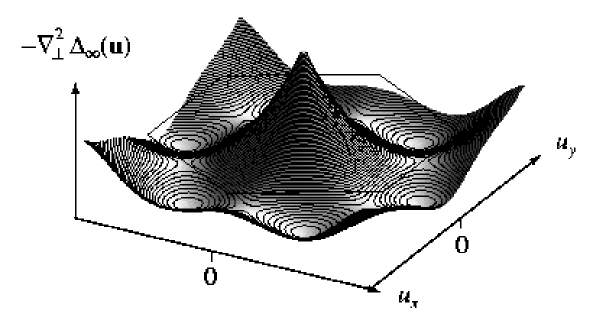
Figure 8: Illustration of the pinning-force correlator $-{\mbox{\boldmath${{\nabla}}$}}_{\perp}^{2}\Delta_{\infty}({\bf u})$ at the RG fixed point after [Emig et al. 1999] (?). The cusp-like non-analyticity at ${\bf u}={\bf 0}$ is a characteristic of the Bragg-glass phase. The hexagon represents the Wigner-Seitz cell of the vortex lattice.

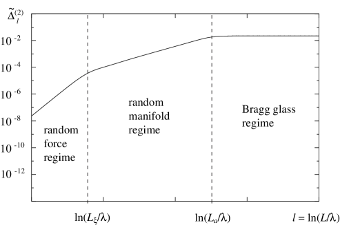
Figure 9: RG flow of $\widetilde{\Delta}^{(2)}_{l}$ through three regimes [Emig et al. 1999]: The random-force regime with a roughness exponent $\zeta_{\rm rf}=(4-d)/2$ for length scales $L\lesssim L_{\xi}$, the random-manifold regime with a non-universal exponent $\zeta_{\rm rm}\approx(4-d)/6$ for length scales $L_{\xi}\lesssim L<\lesssim L_{a}$, and the asymptotic Bragg-glass regime with logarithmic roughness is reached for $L\gtrsim L_{a}$. For weak disorder and $\xi\ll a$, the width of the crossover regions is small compared to the width of the regimes.

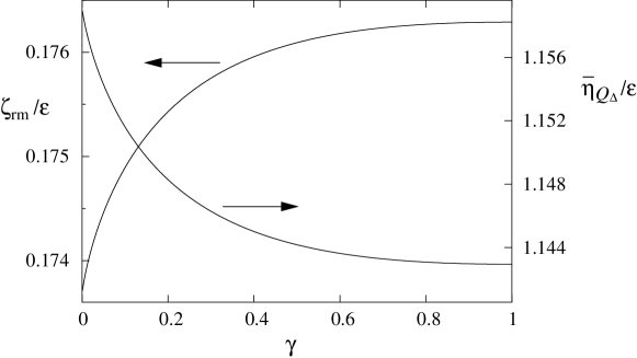
Figure 10: Non-universal variation of the roughness exponents $\zeta_{\rm rm}$ of the random-manifold regime and the correlation function exponent $\bar{\eta}_{\bf Q_{\triangle}}$ with anisotropy parameter $\gamma=c_{66}/c_{11}$ [Emig et al. 1999].

With the numerical value for $\widetilde{\Delta}^{(2)}_{\infty}$ at hands, the explicit form of the displacement correlations

$$W_{\alpha\beta}({\bf r})=\overline{\langle[u_{\alpha}({\bf r})-u_{\alpha}({\bf 0})][u_{\beta}({\bf r})-u_{\beta}({\bf 0})]\rangle}$$ (6.29)

in the Bragg-glass phase is given by [Emig et al. 1999]

$$W_{11}({\bf r}) = \frac{\widetilde{\Delta}^{(2)}_{\infty}(\gamma)a_{\triangle}^{2}}{1+\gamma}\Bigg{\{}\ln\!\left(\frac{x^{2}+z_{t}^{2}}{L_{a}^{2}}\right)+\gamma\ln\!\left(\frac{x^{2}+z_{l}^{2}}{L_{a}^{2}}\right)$$ (6.30a)

$$+\frac{x_{2}^{2}-x_{1}^{2}}{x^{2}}\left[1-\gamma-\frac{z_{t}^{2}}{x^{2}}\ln\!\left(\!1+\frac{x^{2}}{z_{t}^{2}}\!\right)+\gamma\frac{z_{l}^{2}}{x^{2}}\ln\!\left(\!1+\frac{x^{2}}{z_{l}^{2}}\!\right)\right]\!\!\Bigg{\}},\quad\quad$$

$$W_{12}({\bf r}) = \frac{2\widetilde{\Delta}^{(2)}_{\infty}(\gamma)a_{\triangle}^{2}}{1+\gamma}\frac{x_{1}x_{2}}{x^{2}}\Bigg{\{}\gamma-1-\gamma\frac{z_{l}^{2}}{x^{2}}\ln\left(1+\frac{x^{2}}{z_{l}^{2}}\right)$$ (6.30b)

$$+\frac{z_{t}^{2}}{x^{2}}\ln\left(1+\frac{x^{2}}{z_{t}^{2}}\right)\Bigg{\}},$$

and $W_{22}({\bf r})$ follows from $W_{11}({\bf r})$ by permuting $\tilde{c}_{11}$ and $\tilde{c}_{66}$. To lowest order in $\epsilon=4-d$, these correlations lead to the translational order correlation function

$$S({\bf Q},{\bf r}) \equiv \overline{\langle\exp(-i{\bf Q}\cdot[{\bf u}({\bf r})-{\bf u}({\bf 0})])\rangle}$$ (6.31)

$$\sim g_{\bf Q}L_{a}^{\bar{\eta}_{\bf Q}}(x^{2}+z_{t}^{2})^{-\frac{\bar{\eta}_{\bf Q}}{2(1+\gamma)}}(x^{2}+z_{l}^{2})^{-\frac{\bar{\eta}_{\bf Q}}{2(1+1/\gamma)}}$$

with the non-universal $\gamma$-dependent exponent

$$\bar{\eta}_{\bf Q}=\widetilde{\Delta}^{(2)}_{\infty}(\gamma)(a_{\triangle}Q)^{2}$$ (6.32)

and the geometrical prefactor

$$g_{\bf Q} = \exp\left\{\frac{\widetilde{\Delta}^{(2)}_{\infty}(\gamma)(a_{\triangle}Q)^{2}}{1+\gamma}\left[(\hat{\bf x}\cdot\hat{\bf Q})^{2}-\frac{1}{2}\right]\!\,\right.$$ (6.33)

$$\times\,\left.\left[\!\left(\!1-\frac{z_{t}^{2}}{x^{2}}\ln\!\left(\!1+\frac{x^{2}}{z_{t}^{2}}\right)\!\!\right)-\gamma\left(\!1-\frac{z_{l}^{2}}{x^{2}}\ln\!\left(\!1+\frac{x^{2}}{z_{l}^{2}}\right)\!\!\right)\!\right]\right\},$$

which completely describes the angular dependencies of the translational order. Note that the factor $g_{\bf Q}$ goes to $1$ in the limit $z\to\infty$. Therefore, in this limit the dependence of $S({\bf Q},{\bf r})$ on the reciprocal lattice vector ${\bf Q}$ remains only in the exponent $\bar{\eta}_{\bf Q}$. Moreover, it is interesting to note that the exponents of the algebraic decay in equation (6.31) depend on the elastic moduli as soon as $z$ is finite even without taking into account the non-universality of the exponent $\bar{\eta}_{\bf Q}$ itself. If one ignores the non-trivial $\gamma$ dependence of $\bar{\eta}_{\bf Q}$, in the case $z=0$ the above formulas reduce to those found in [Giamarchi and Le Doussal 1994] (?, ?). A logarithmic roughness of $W({\bf r})$ was already predicted earlier from scaling arguments [Nattermann 1990] and found also from a variational treatment with replica-symmetry breaking by [Korshunov 1993] (?) and [Giamarchi and Le Doussal 1994] (?, ?). However, this method is not able to capture the non-universality of $\bar{\eta}_{\bf Q}$.

The $\gamma$-dependence of the exponent $\bar{\eta}_{\bf Q_{\triangle}}$ for a smallest reciprocal lattice vector $Q_{\triangle}$ is depicted in figure 10 and varies numerically from $\bar{\eta}_{\bf Q_{\triangle}}=1.143$ for $\gamma=0$ to $\bar{\eta}_{\bf Q_{\triangle}}=1.159$ for $\gamma=1$. In isotropic superconductors at low temperatures, where vortex lines interact via central forces, one has $0\leq\gamma\leq 1/3$. $\gamma\sim 1/3$ for $\lambda\leq a$, i.e., for fields close to $H_{\rm c1}$, and $\gamma\rightarrow 0$ for $H\rightarrow H_{\rm c2}$. For most of the field region $\gamma\approx\Phi_{0}/16\pi\lambda^{2}B$. Thus, an increase of the external field from $H_{\rm c1}$ to $H_{\rm c2}$ should result in an increase of $\bar{\eta}_{\bf Q}$ and a decrease of $\zeta_{\rm rm}$. At higher temperatures, where the vortex line interaction is renormalized considerably by thermal fluctuations, as well as in anisotropic superconductors, the above inequality for $\gamma$ may no longer be fulfilled. Clearly, in the latter case our starting Hamiltonian (6.22) would also have to be modified.

The non-universality of $\bar{\eta}_{\bf Q}$ could, in principle, be tested by neutron scattering experiments at changing external fields. On the experimental side, Bragg peaks have indeed been observed in BSCCO for $H\lesssim 500$G by [Cubitt et al. 1993] (?). More recently, [Kim et al. 1999] (?) have used the decoration technique to determine the structural properties of the vortex lattice in BSCCO and confirmed the existence of the perturbative and the random-manifold regime with $\zeta_{\rm rf}\approx 0.22$. On larger length scales their data exhibited non-equilibrium features such that the true asymptotic regime was not reached. So far, the resolution is, however, too weak to determine the $\gamma$ dependence of $\bar{\eta}$. Contact to the neutron scattering experiment can be made by the structure factor

$$\widehat{S}({\bf k}_{\perp},k_{z}) = \sum_{\bf X}\int dz\ \overline{\langle e^{i{\bf k}_{\perp}\cdot[{\bf X}+{\bf u}({\bf X},z)-{\bf u}({\bf 0},0)]+ik_{z}z}\rangle}$$ (6.34)

$$\approx \sum_{\bf X}\int dz\ e^{i({\bf k}_{\perp}\cdot{\bf X}+k_{z}z)}e^{-\frac{1}{2}k_{\alpha}k_{\beta}W_{\alpha\beta}({\bf X},z)},$$

where we have used the Gaussian approximation (which is correct to order $\epsilon$) for the distribution of ${\bf u}$ and the definition (6.29) for $W_{\alpha\beta}$. With ${\bf k}_{\perp}={\bf Q}+{\bf q}_{\perp}$ and $|{\bf q}_{\perp}|\ll|{\bf Q}|$ we get

$$\widehat{S}({\bf Q}+{\bf q}_{\perp},k_{z})\approx\rho_{0}\int d^{3}r\ e^{i({\bf q}_{\perp}\cdot{\bf x}+k_{z}z)}S({\bf Q},{\bf r}).$$ (6.35)

$\widehat{S}({\bf k})$ describes the divergence of the scattered intensity with vanishing ${\bf q}$ in the vicinity of a reciprocal lattice vector ${\bf Q}$. The above integral is dominated for small ${\bf q}$ by the large scale $S({\bf Q},{\bf r})$, provided $\bar{\eta}_{\bf Q}(\gamma)<3$. It is thus the sub-algebraic growth of the displacements (LABEL:displace_ab) that gives rise to the Bragg peaks, hence the name ‘Bragg glass’. In the special cases $\gamma=0$ and $\gamma=1$ one obtains

$$\widehat{S}({\bf Q}+{\bf q}_{\perp},k_{z})\sim\left(q_{\perp}^{2}+\frac{c_{44}}{c_{66}}k_{z}^{2}\right)^{[-3+\bar{\eta}_{\bf Q}(\gamma)]/2}.$$ (6.36)

To summarize the situation in impure bulk superconductors: it turns out that these still show a quasi-long-range ordered ‘Bragg-glass’ phase which is described by a non-universal power-like decay of the order parameter correlations. In particular, the decay-exponent $\bar{\eta}_{\bf Q}$ depends on the ratio $\gamma={\tilde{c}}_{66}/{\tilde{c}}_{11}$ of the elastic constants, similar to $2D$ pure crystals at their melting temperature. For weak disorder we find a crossover of the structural correlation functions $S({\bf Q},{\bf r})$ from a Larkin regime, where perturbation theory applies and $S({\bf Q},{\bf r})$ decays exponentially, to the random-manifold regime with a stretched exponential decay of $S({\bf Q},{\bf r})$ and eventually to the asymptotic Bragg-glass regime.

In addition to the disorder-averaged positional correlation function $S({\bf Q},{\bf r})$ it is interesting to also consider the glass correlation functions $S_{\rm PG}({\bf Q},{\bf r})$ and $C_{\rm VG}({\bf Q},{\bf r})$. In the framework of the functional RG in $d=4-\epsilon$ dimensions, discussed above, it is easy to show that to first order $\epsilon$ one finds [Bogner et al. 2000]

$$S_{\rm PG}({\bf Q},{\bf r})\approx S_{\rm PG}^{(0)}({\bf Q},{\bf r})\left[1+\epsilon\sum_{m\geq 1}c_{m}\left(\frac{T}{r^{2}}\right)^{2m}+O(\epsilon^{2})\right],$$ (6.37)

where $S_{\rm PG}^{(0)}({\bf Q},{\bf r})=[S^{(0)}({\bf Q},{\bf r})]^{2}$. $S^{(0)}({\bf Q},{\bf r})=\exp[-\frac{1}{2}Q_{\alpha}Q_{\beta}W_{{\rm th},\alpha\beta}({\bf r})]$ denotes the pair-correlation function for TLRO of the pure system, which is finite for $r\to\infty$ if $d>2$ and is reduced with respect to unity merely by the standard Debye-Waller factor. For large distances $|{\bf r}|$ the leading correction in (6.37) comes from the term with $m=1$. Since $c_{1}>0$, the disorder increases slightly the glass order with respect to the pure system as has to be expected. With $S_{\rm PG}({\bf Q},{\bf r})/[S({\bf Q},{\bf r})]^{2}\to\infty$ for $r\to\infty$, we conclude that the Bragg-glass regime is indeed a positional glass. Using the relation (2.25) it is also easy to show to order $\epsilon$ that $C_{\rm VG}({\bf r})$ decays exponentially in $d<4$ dimensions (and algebraically for $d=4$). Expanding all corrections from the disorder with respect to $\epsilon=4-d$ we get

$$C_{\rm VG}({\bf r})\approx e^{-\frac{1}{2}\langle(\delta\phi({\bf r})-\delta\phi({\bf 0}))^{2}\rangle_{\rm th}}\left[1+\epsilon\sum_{m\geq 0}\tilde{c}_{m}T^{2}\left(\frac{T}{r}\right)^{2m}+O(\epsilon^{2})\right],$$ (6.38)

where

$$\langle(\delta\phi({\bf r})-\delta\phi({\bf 0}))^{2}\rangle_{\rm th}=2\left(\frac{2\pi}{a^{2}}\right)^{2}T\int_{\bf q}\frac{q_{\perp}^{2}[1-\cos({\bf q}\cdot{\bf x})]}{q^{4}(c_{66}q_{\perp}^{2}+c_{44}q_{\parallel}^{2})}\sim\frac{1}{\epsilon}|{\bf x}|^{\epsilon}$$ (6.39)

denotes the phase fluctuations of the order parameter in the pure system (see [Moore 1992] (?)). Although the leading correction ($m=0$) from the disorder increases $C_{\rm VG}({\bf r})$, it does not compensate its exponential decay originating from strong thermal fluctuations in the pure system. Whether this result remains qualitatively correct if higher order terms in $\epsilon$ are taken into account remains an open question. For the moment we conclude that to order $\epsilon$ there is no phase-coherent vortex-glass order in the Bragg-glass phase.

Our findings are not necessarily in contradiction to the result of [Dorsey et al. 1992] (?) who, starting from a random-$T_{\rm c}$ GL model and using mean-field theory, found a transition to a phase with phase-coherent glass order. However, this calculation – once fluctuations are taken into account – proves the existence of a vortex glass transition with a diverging susceptibility $\chi_{\rm VG}=\int d^{d}r\ C_{\rm VG}({\bf r})$ only in $d=6-\epsilon$ dimensions ($\epsilon\ll 1$). In this region ($d>4$) our calculation also gives both $S_{\rm PG}({\bf Q},{\bf r})$ and $C_{\rm VG}({\bf r})$ non-zero for $r\to\infty$.

6.3 Stability of Bragg glass

In this chapter we have been treating so far the vortex-line lattice in the elastic approximation, i.e., we have disregarded topological defects such as dislocations or disclinations.

In the following we will consider the stability of the Bragg-glass phase with respect to dislocations. This problem was considered by several authors [Giamarchi and Le Doussal 1995, Kierfeld et al. 1997, Gingras and Huse 1996, Carpentier et al. 1996, Ertaş and Nelson 1996, Giamarchi and Le Doussal 1997, Fisher 1997, Kierfeld 1998, Koshelev and Vinokur 1998]. Since the disorder seen by the dislocation is already partially screened due to the elastic deformations (a fact which was overlooked in the early discussion of the elastic approximation by [Fisher et al. 1991a] (?)), we start this section with a brief discussion of the effective disorder strength $\widetilde{\Delta}_{\rm eff}(R)$ acting on scale $R$ in the various regimes. We will thereby ignore all numerical coefficients of order unity and restrict ourselves to the case $d=3$.

For simplicity, we restrict ourselves here to the case $c_{11}\gg c_{66}$ such that we can assume ${\mbox{\boldmath${{\nabla}}$}}_{\perp}\cdot{\bf u}=0$. It is then convenient to rewrite the Hamiltonian using the coordinate $z_{t}=({c_{66}/c_{44}})^{1/2}z$ introduced in equation (6.10). The elastic part of the Hamiltonian is now isotropic with $c_{44}$ and $c_{66}$ replaced by their geometric mean $({c_{44}c_{66}})^{1/2}$. The same transformation in the pinning part changes $\widetilde{\Delta}({\bf u})$ into $({c_{44}/c_{66}})^{1/2}\widetilde{\Delta}({\bf u})$. It is also convenient to introduce the (anisotropic) distance $R_{t}$,

$$R_{t}^{2}={\bf x}^{2}+z_{t}^{2}.$$ (6.40)

$\widetilde{\Delta}^{(2)}_{\rm eff}(R)$ was introduced already in equation (6.28). We use here (6.27) to find explicit expressions for the mean square displacement $\overline{{\bf u}^{2}}(R_{t})$. To obtain an estimate for $\overline{{\bf u}^{2}}(R_{t})\approx W(R_{t})/2$ on the scale $R_{t}$ one equates the elastic energy $E_{\rm el}\approx({c_{44}c_{66}})^{1/2}\ \overline{{\bf u}^{2}}R_{t}$, with the fluctuation of the pinning energy

$$E_{\rm pin}\approx\left(\frac{c_{44}}{c_{66}}\right)^{1/4}R_{t}^{3/2}\left(\widetilde{\Delta}^{(2)}_{\rm eff}(R_{t})\overline{{\bf u}^{2}}\right)^{1/2}.$$ (6.41)

$\widetilde{\Delta}^{(2)}_{\rm eff}(R_{t})$ denotes the curvature of the effective potential correlator at ${\bf u}=0$ on the length scale $R_{t}$. The estimate for the pinning energy corresponds to the use of perturbation theory applied on the renormalized random potential. In this way we obtain

$$\overline{{\bf u}^{2}}\approx c_{44}^{-1/2}c_{66}^{-3/2}\widetilde{\Delta}^{(2)}_{\rm eff}(R_{t})R_{t}=\xi^{2}\frac{\widetilde{\Delta}^{(2)}_{\rm eff}(R_{t})}{\widetilde{\Delta}^{(2)}}\frac{R_{t}}{R_{\xi}},$$ (6.42)

where $\widetilde{\Delta}^{(2)}\equiv\widetilde{\Delta}^{(2)}(R_{\xi})$ denotes the bare value of $\widetilde{\Delta}^{(2)}(R_{t})$.

Now we consider the different regimes already discussed in section 6.2.

(i) In the perturbative regime $R_{t}<R_{\xi}\approx\xi^{2}c_{44}^{1/2}c_{66}^{3/2}/\widetilde{\Delta}^{(2)}$, $\widetilde{\Delta}^{(2)}_{\rm eff}\approx\widetilde{\Delta}^{(2)}$ in equation (6.42).

(ii) In the manifold region, $R_{\xi}<R_{t}<R_{a}$, where $\overline{{\bf u}^{2}}\approx\xi^{2}(R_{t}/R_{\xi})^{2\zeta_{\rm rm}}$, we find from equation (6.42)

$$\widetilde{\Delta}^{(2)}_{\rm eff}(R_{t})\approx\widetilde{\Delta}^{(2)}\cdot\left(\frac{R_{t}}{R_{\xi}}\right)^{2\zeta_{\rm rm}-1}.$$ (6.43)

(iii) Finally, in the asymptotic Bragg-glass region, $R_{a}<R_{t}$, we get from $\overline{{\bf u}^{2}}\approx a^{2}\ln(R_{t}/R_{a})$

$$\widetilde{\Delta}^{(2)}_{\rm eff}(R_{t})\approx\widetilde{\Delta}^{(2)}\frac{R_{\xi}}{R_{t}}\frac{a^{2}}{\xi^{2}}\approx\frac{a^{2}c_{44}^{1/2}c_{66}^{3/2}}{R_{t}}.$$ (6.44)

Thus, $\widetilde{\Delta}^{(2)}_{\rm eff}(R_{t})$ is independent of the bare disorder strength. Here we have to ignore the logarithm since it originates from the summation over many different length scales.

We use now these expressions to obtain an estimate for the energy of a dislocation loop. For simplicity, we assume an isotropic (i.e., almost circular) loop of linear size $R_{t}$. In the pure system, its elastic energy is

$$E_{\rm el}^{\rm loop}\approx b^{2}(c_{44}c_{66})^{1/2}R_{t}\ln(R_{t}/a_{1}),$$ (6.45)

where $|{\bf b}|=a_{\triangle}$ and ${\bf b}$ denotes the Burgers vector of the dislocation. The logarithm results from the fact that in a distance $R_{t}$ from the dislocation centre the displacement ${\bf u}_{\rm disloc}$ produced by the dislocation line obeys $|{\mbox{\boldmath${{\nabla}}$}}\wedge{\bf u}_{\rm disloc}|\sim\frac{|{\bf b}|}{2\pi R_{t}}$. Integration over the plane perpendicular to the dislocation line then yields $\sim a_{\triangle}^{2}(c_{44}c_{66})^{1/2}\ln(R_{t}/a_{1})$ for the energy per unit length, where $a_{1}$ acts as a small distance cut-off.

In a random system, the situation is more complicated. Since the displacement ${\bf u}_{\rm disloc}$ created by a dislocation line obeys the saddle-point equation $\delta{\cal H}/\delta{{\bf u}}=0$ as well as $\oint d{\bf u}={\bf b}$, the elastic energy of the dislocation now depends also on the disorder. Since the situation apparently is rather involved, we will adopt here a simplified picture using the following observation: The displacement in the neighbourhood of a dislocation has two sources: Its very existence leads in the distance $R_{t}$ from the dislocation to a (essentially tangential) displacement of order $a$. The disorder, on the other hand, creates displacements (both in the absence or in the presence of a dislocation) of order $a$ or larger only on scales $R_{t}>R_{a}$. In calculating the energy of a loop of linear size $R_{t}>R_{a}$ in the disordered case we estimate the elastic energy of the dislocation loop therefore by

$$E_{\rm el}^{\rm loop}\approx a^{2}(c_{44}c_{66})^{1/2}R_{t}\ln(R_{a}/a_{1}),$$ (6.46)

since distortions originating from the random potential are small compared to $a$ on scales $R\lesssim R_{a}$ but are dominating on larger scales. So far we have ignored the dispersion of the elastic constant $c_{44}$, which becomes relevant on scales small compared to $\lambda$. On these scales the lattice is softer by a factor $(R_{t}/\lambda)^{2}$. In order to take this effect into account, we replace the small scale cut-off $a_{1}$ in (6.46) by $(a_{1}^{2}+\lambda^{2})^{1/2}$.

The distortions on scales larger than $R_{a}$ are dominated by the disorder and lead to an energy gain of the order (again omitting the factor $\ln(R_{t})$ in $\overline{{\bf u}^{2}}$, since it comes from the summation over displacements on different length scales)

$$E_{\rm pin}^{\rm loop}\approx-\left(\frac{c_{44}}{c_{66}}\right)^{1/4}R_{t}^{3/2}\left(\widetilde{\Delta}^{(2)}_{\rm eff}\ \overline{{\bf u}^{2}}\right)^{1/2}\approx-a^{2}(c_{44}c_{66})^{1/2}R_{t}$$ (6.47)

where we used equations (6.41) and (6.44). The total loop energy of a dislocation loop can therefore be written as

$$E^{\rm loop}\approx a^{2}(c_{44}c_{66})^{1/2}R_{t}\left(\ln\left(\frac{R_{a}^{2}}{a_{1}^{2}+\lambda^{2}}\right)-c_{1}\right),$$ (6.48)

where $c_{1}$ is a constant of order unity. (It is easy to see by analogous arguments, but using equations (6.42) or (6.43) for $\Delta_{\rm eff}(R_{t})$, that dislocation loops of size $R_{t}<R_{a}$ always have a positive energy.)

From (6.48) we conclude that the system is stable against the formation of a dislocation loop as long as

$$R_{a}\gtrsim c_{2}(a_{1}^{2}+\lambda^{2})^{1/2}$$ (6.49)

with $c_{2}\approx e^{c_{1}}$. As shown by [Kierfeld 1998] (?) for strong disorder (i.e., $R_{\xi}\leq a$), this relation can be rewritten in the form of a Lindemann criterion. Indeed, in the manifold regime (note that the Larkin regime vanishes for strong disorder), where

$$\frac{\overline{{\bf u}^{2}}(R_{a})}{\overline{{\bf u}^{2}}(a)}\approx\left(\frac{R_{a}^{2}}{a^{2}+\lambda^{2}}\right)^{\zeta_{\rm rm}}$$ (6.50)

and $\overline{{\bf u}^{2}}(R_{a})\approx a^{2}$ one obtains from (6.49)

$${\overline{\langle[{\bf u}(a)-{\bf u}(0)]^{2}\rangle}}^{1/2}\lesssim c_{\rm Li}\ a,$$ (6.51)

which is the Lindemann criterion appropriate for disordered systems in which the mean-square displacement of a single vortex line diverges. $c_{\rm Li}=c_{2}^{-\zeta_{\rm rm}}$ denotes the Lindemann number. The main conclusion from this consideration is that the elastic, dislocation-free Bragg glass is stable as long as the criterion (6.49) or, for strong disorder, equation (6.51)] is fulfilled.

A few concluding remarks are in order:

• The criterion (6.51) [or, equivalently, equation (6.49)] was also derived by [Kierfeld et al. 1997] (?) and [Carpentier et al. 1996] (?) via a variational treatment for a layered system with the magnetic field parallel to the layers. In this model only dislocations with Burgers vectors parallel to the layers are allowed. The most important result is the determination of the Lindemann number $c_{\rm Li}\approx 0.14$. We refer the reader to these papers for further details.

• [Ertaş and Nelson 1996] (?) took equation (6.51) as a starting point for a discussion of the onset of irreversibility and entanglement of vortex lines in high-$T_{c}$ materials.

• [Kierfeld 1998] (?), on the basis of equation (6.51), and including the dispersion of the elastic constants in detail, calculated the stability boundaries of the Bragg-glass phase for YBCO and BSCCO. The resulting phase diagram is depicted schematically in figure 11. Since the shear modulus decreases for large and small fields, respectively, there are two corresponding stability boundaries.

• [Fisher 1997] (?) undertook a much more detailed study of the stability of a defect loop in the random-field $XY$ model which corresponds to the layered model mentioned in (i). Although the details of his energy estimate for the dislocation loop are slightly different from those presented here (using a statistical tilt symmetry, he estimates $E_{\rm el}^{\rm loop}$ by equation (6.45) but includes also rare fluctuations in the energy gain from the disorder, which also include logarithmic corrections), his final conclusions concerning the stability of the defect-free phase are essentially identical to those presented here.

• [Ryu et al. 1996b] (?) numerically investigated the field-driven transition from a dislocation-free to a dislocation-dominated phase in an impure layered superconductor and found good quantitative agreement with the estimates made above as well as with the neutron-scattering data of [Cubitt et al. 1993] (?), who found the disappearance of Bragg peaks in BSCCO for $H\gtrsim$500G.

• Most recently, [Kierfeld and Vinokur 1999] (?) used a random-stress model of the form (3.33) as an effective model to describe dislocation lines in an impure superconductor. The correlations of the random-stress field ${\mbox{\boldmath${{\mu}}$}}({\bf r})$ on different length scales are chosen in such a way that the correct roughness exponents in the manifold and the Bragg-glass regime, respectively, are reproduced. Considering in particular dislocation lines with main orientation parallel to the magnetic field, which enter and leave the sample at its surface, [Kierfeld and Vinokur 1999] (?) found a global phase diagram, which includes – besides the elastic Bragg-glass phase with vanishing dislocation density – an amorphous vortex-glass and a vortex-liquid phase separated by a first-order transition line which terminates in a critical point (see figure 11).

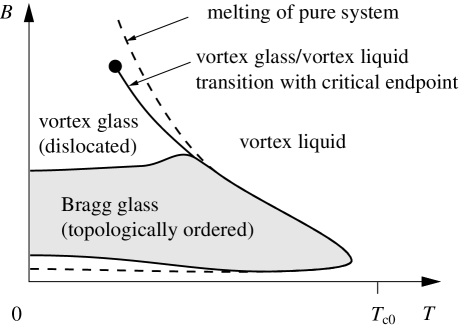
Figure 11: Schematic phase diagram of the vortex system according to [Kierfeld 1998] (?) and [Kierfeld and Vinokur 1999] (?). In the absence of disorder the vortex lattice melts into the vortex liquid at low and high magnetic fields (dashed line). Due to the presence of disorder the vortex lattice becomes the Bragg glass in a reduced stability region (shaded area), where the system is stable to the proliferation of dislocations. At low temperatures and low or high fields, disorder induces the proliferation of dislocations for energetic reasons and the phase becomes the vortex glass. The phase transition from the vortex lattice to the vortex liquid has a critical end point.

7 Vortices driven far from equilibrium

As the main result of the previous chapter we found that weak pinning reduces the positional order of the vortex lattice in a bulk superconductor from long-range order to quasi-long-range order. The discussion was restricted to thermodynamic equilibrium. However, since the electric resistivity is one of the most relevant physical properties of superconductors, it is important to study the driven non-equilibrium situation. Since the efficiency of pinning is related to the structure of the vortex system, it is of particular interest to characterize this structure. In addition, since the melting transition of the vortex lattice shows up as a pronounced shoulder in the transport characteristic (see, e.g., [Safar et al. 1992] (?), [Kwok et al. 1992] (?)), it is desirable to locate this transition in the non-equilibrium situation.

The VLL shows the three regimes of creep, depinning, and flow in its transport characteristic, which were already described for manifolds in chapter 3.2 (cf. figure 5). We recall that in a superconductor the vortex velocity is proportional to the electric field and the driving force is proportional to the electric current density. So far, we have mainly focused on the creep regime when we addressed transport properties in the previous chapters. In this regime, which is close to equilibrium, the dynamical response is determined within the scaling approach by the structure of the VLL in equilibrium. In particular, the logarithmic roughness of the elastic vortex glass (described by a roughness exponent $\zeta=0$) results in a drift velocity

$$v(F)\sim(F/\eta_{0})\ e^{-U(F)/T},$$ (7.1)

where the effective barrier height $U(F)$ scales with the driving force $F$ according to

$$U(F)\sim F^{-\mu}$$ (7.2)

with the creep exponent [Nattermann 1990]

$$\mu=\frac{d-2}{2}$$ (7.3)

[cf. equations (3.71) to (3.73) with the appropriate substitution for the dimension of the manifold]. In $d<2$ one thus expects $\mu<0$, which means that the system has a linear transport characteristic at small driving forces. Only in $d\geq 2$ we can expect to find true superconductor with a vanishing linear resistivity. The ($d=2$)-dimensional case is marginal since it has the creep exponent $\mu=0$. There the effective barrier height depends logarithmically on the driving force and results in a power-law transport characteristic as found in equations (4.56) and (5.30) for the superconducting film in parallel and perpendicular field.

In this chapter we will focus on the flow regime, which is far from equilibrium but accessible to a theoretical analysis because it is, roughly speaking, close to the pure case since disorder is dynamically ‘averaged out’. We will elucidate this point later on. Although the flow regime might appear to be of no special interest at first sight, only recently it turned out to be quite non-trivial, including phenomena such as non-equilibrium phase transitions.

To perform the theoretical analysis of a stationary state at average velocity ${\bf v}$ it is convenient to define the displacement ${\bf u}({\bf X},{\bf z},t)\equiv{\bf x}({\bf X},{\bf z},t)-{\bf X}-{\bf v}t$ by subtracting the average temporal displacement, such that ${\bf u}$ still can be considered as a small quantity. ${\bf X}$ is then the ideal vortex position measured in a frame moving with velocity ${\bf v}$. In analogy to manifolds, the equation of motion for the vortex lattice,

$$\eta_{0}\dot{\bf u}={\bf F}^{\rm int}+{\bf F}^{\rm pin}+{\bf F}-\eta_{0}{\bf v}+{\mbox{\boldmath${{\zeta}}$}},$$ (7.4)

is over-damped. In comparison to equation (3.53) for a single vortex line, equation (7.4) includes the vortex density $\rho_{0}$ as additional factor, such that the latter equation is an equation for the force density in the $d$-dimensional space. Accordingly, the left-hand side is the Bardeen-Stephen friction force $\eta_{0}\dot{\bf u}$ [Bardeen and Stephen 1965], with the friction coefficient $\eta_{0}\approx BH_{\rm c2}/\rho_{\rm n}c^{2}$ referring to the force per unit volume, whereas the previous expression (3.50) refers to the force per unit length of a vortex line. ${\bf F}^{\rm int}$ is the force acting on a vortex due to its interaction with other vortices. In a harmonic approximation for the elastic phase one has ${\bf F}^{\rm int}\approx{\bf F}^{\rm el}$. The instantaneous elastic force ${\bf F}^{\rm el}$ depends linearly on ${\bf u}$ and reads

$$F^{\rm el}_{\alpha}({\bf q},t) = \Gamma_{\alpha\beta}({\bf q})u_{\beta}({\bf q},t),$$ (7.5a)

$$\Gamma_{\alpha\beta}({\bf q}) = \sum_{p}[c_{p}q_{\perp}^{2}+c_{44}q_{\parallel}^{2}]P^{p}_{\alpha\beta}({\bf q}_{\perp}),$$ (7.5b)

where $\Gamma$ represents the elastic dispersion, $p=L,T$ stands for the longitudinal/transverse polarization, $c_{p}\equiv c_{11},c_{66}$ respectively, and $q_{\perp}^{2}=q_{x}^{2}+q_{y}^{2}$. As far as we consider a general dimension $d$, ${\bf x}$ and ${\bf q}_{\perp}$ are two-dimensional and ${\bf z}$ and ${\bf q}_{\parallel}$ are $(d-2)$-dimensional. ${\bf F}^{\rm pin}$ is the pinning force density

$${\bf F}^{\rm pin}({\bf X},{\bf z},t)=-\rho_{0}{\mbox{\boldmath${{\nabla}}$}}_{\perp}V({\bf X}+{\bf v}t+{\bf u}({\bf X},{\bf z},t),{\bf z}),$$ (7.6)

which implicitly depends on the displacement ${\bf u}$. The pinning potential $V$ and the thermal noise ${{\zeta}}$ are assumed to be Gaussian distributed with correlators (6.2) and

$$\langle\zeta_{\alpha}({\bf X},{\bf z},t)\zeta_{\beta}({\bf 0},{\bf 0},0)\rangle=2\eta_{0}T\rho_{0}\ \delta_{{\bf X},{\bf 0}}\ \delta_{\alpha\beta}\delta({\bf z})\delta(t)$$ (7.7)

in analogy to equation (3.52).

7.1 Qualitative aspects

On the basis of this equation of motion we can become more specific in what sense disorder is ‘dynamically averaged out’ in the limit of large drift velocities. In this limit the pinning force ${\bf F}^{\rm pin}({\bf X},{\bf z},t)$ acting on a fixed vortex element at position $({\bf X},{\bf z})$ in the comoving frame changes rapidly as a function of time. Since the VLL has finite response times on finite length scales, the displacements induced by the pinning force decrease with increasing ${\bf v}$ and the pinning potential is effectively averaged (‘washed’) out. Therefore the effect of disorder vanishes in the limit of very large driving force.

To substantiate this relation it is instructive to consider a single vortex line ${\bf X}$ moving with strictly constant velocity (i.e., ${\bf x}={\bf X}+{\bf v}t$), neglecting its response to pinning. In this approximation the vortex line experiences a time dependent force ${\bf F}^{\rm pin}({\bf X},{\bf z},t)=-\rho_{0}{\mbox{\boldmath${{\nabla}}$}}_{\perp}V({\bf X}+{\bf v}t,{\bf z})$. To some extent the effect of this force can be compared to an additional thermal noise with a certain ‘shaking temperature’ $T^{\rm sh}$. We choose the ${\bf x}\equiv(x,y)$ coordinates such that ${\bf v}=(v,0)$ points into the direction of the first basis vector ${\bf e}_{x}$. Then

$$T^{\rm sh}_{\alpha} \equiv \frac{1}{2\eta_{0}\rho_{0}}\int dtd^{d-2}z\ \overline{F^{\rm pin}_{\alpha}({\bf X},{\bf z},t)F^{\rm pin}_{\alpha}({\bf X},{\bf 0},0)}$$ (7.8a)

$$= -\frac{\rho_{0}}{2\eta_{0}v}\int dx_{1}\ \partial_{\alpha}^{2}\Delta(x_{1}{\bf e}_{x}),$$

$$T^{\rm sh}_{x} = 0,$$ (7.8b)

$$T^{\rm sh}_{y} \simeq \frac{\rho_{0}\Delta_{0}}{2\eta_{0}v\xi^{3}},$$ (7.8c)

where $\alpha=x,y$ is not to be summed over implicitly. These equations are strictly analogous to the equations (LABEL:T.sh.mani) for manifolds.

The concept of the ‘shaking temperature’ was introduced by [Koshelev and Vinokur 1994] (?), who considered in particular the case $d=2$ and introduced the ‘incoherent’ shaking temperature $T^{\rm sh}\equiv\frac{1}{2}\sum_{\alpha}T^{\rm sh}_{\alpha}$. For qualitative purposes they considered the system driven through disorder as being subject to a total effective temperature $T_{\rm eff}(v)=T+T^{\rm sh}(v)$. Then the vortex lattice can be expected to melt at a velocity-dependent temperature

$$T_{\rm m}(v)=T_{\rm m}-T^{\rm sh}(v),$$ (7.9)

where $T_{\rm m}\equiv T_{\rm m}(v=\infty)$ is the melting temperature of the pure system. Equivalently, the inverted function $v_{\rm m}(T)$ defines a melting velocity above which the vortices freeze into a solid (‘dynamic freezing’). $T^{\rm sh}$ vanishes for increasing $v$ and hence both $v_{\rm m}$ and the corresponding driving force $F_{\rm m}=F(v_{\rm m})$ increase with increasing $T$ for fixed pinning strength. From the velocity dependence of $T^{\rm sh}_{y}$ one expects

$$T_{\rm m}-T_{\rm m}(v)\propto\frac{1}{v}\propto\frac{1}{F}$$ (7.10)

at large driving forces. This relation is consistent with experimental observations [Bhattacharya and Higgins 1993, Hellerqvist et al. 1996] and numerical simulations [Koshelev and Vinokur 1994].

A quantitative analysis of the pinning effects requires taking into account the interaction between the vortex lines. For this purpose [Koshelev and Vinokur 1994] (?) introduced a ‘coherent’ shaking temperature, which they found to scale like $T^{\rm sh}_{\rm coh}(v)\approx({v_{\rm rel}}/{v})T^{\rm sh}(v)$ with a characteristic velocity scale $v_{\rm rel}$, taking into account only the transverse response of the VLL in $d=2$. However, the question of what physical properties of the system can be described by such an effective temperature is quite subtle. This is evident from equation (LABEL:intro.Tsh), which shows that the shaking effect is anisotropic and that one should distinguish the direction parallel to the driving force from perpendicular directions.

A more careful treatment of disorder will be presented below to evaluate the effects of disorder on a solid VLL in an elastic approximation (section 7.2) and to characterize the structure of the driven lattice, before one can analyze the stability of the VLL with respect to the proliferation of topological defects, from what one can locate the melting transition (section 7.3).

7.2 Moving lattice

To characterize the structure of the vortex lattice driven in disorder, we start from the assumption of an elastic and topologically ordered phase, as exists in the absence of disorder and for low temperatures in $d\geq 2$. The first step is to treat pinning perturbatively in the high-velocity regime. This analysis is most convenient in Fourier representation, which reads for the displacement

$${\bf u}({\bf r},t)=\int_{\omega}\int_{\bf q}e^{i({\bf q}\cdot{\bf r}-\omega t)}{\bf u}({\bf q},\omega),$$ (7.11)

where $\int_{\omega}=\int d\omega/2\pi$ and $\int_{\bf q}=\int d^{d}q/(2\pi)^{d}$ is restricted to the first Brillouin zone. The dynamic response function $G$ of the pure system is ($p=L,T$)

$$G_{\alpha\beta}({\bf q},\omega) = \sum_{p}G^{p}({\bf q},\omega)P^{p}_{\alpha\beta}({\bf q}),$$ (7.12a)

$$G^{p}({\bf q},\omega) = [-i\eta_{0}\omega+c_{p}q_{\perp}^{2}+c_{44}q_{\parallel}^{2}]^{-1}.$$ (7.12b)

To zeroth order in ${\bf u}$ the pinning force acting on the VLL in the comoving frame has the correlation

$$\Xi_{\alpha\beta}({\bf X},{\bf z},t) \equiv \overline{F^{\rm pin}_{\alpha}({\bf X},{\bf z},t)F^{\rm pin}_{\beta}({\bf 0},{\bf 0},0)}$$ (7.13a)

$$= -\rho_{0}^{2}\partial_{\alpha}\partial_{\beta}\Delta({\bf X}+{\bf v}t)\delta({\bf z}),$$

$$\Xi_{\alpha\beta}({\bf q},\omega) = \rho_{0}^{2}\sum_{\bf Q}k_{\alpha}k_{\beta}\Delta({\bf k})\delta(\omega+{\bf v}\cdot{\bf k})$$ (7.13b)

$$= \rho_{0}^{2}\sum_{\bf Q}\Delta^{(2)}_{\alpha\beta}({\bf k})\delta(\omega+{\bf v}\cdot{\bf k}),$$

where ${\bf Q}$ is a reciprocal lattice vector (RLV) and $\Delta^{(2)}_{\alpha\beta}({\bf k})\equiv k_{\alpha}k_{\beta}\Delta({\bf k})$. The wave vector ${\bf k}\equiv{\bf Q}+{\bf q}$ covers the whole Fourier space without restriction to the first Brillouin zone (in contrast to ${\bf q}$).

In the following we assume that the vortex lattice is oriented with one principal axis parallel to the average velocity. [Schmid and Hauger 1973] (?) argued that the vortex lattice orients itself in this direction because this is the direction of minimum entropy production and of least power dissipation. One can arrive at the same conclusion from a stability analysis [Müllers and Schmid 1995]. In this case there are RLVs ${\bf Q}$ which are perpendicular to the velocity ${\bf v}$ and which play an important role for the dynamics. An inspection of the correlator (LABEL:intro.Xi) for $\omega=0$ and ${\bf q}={\bf 0}$ shows that the disorder correlator evaluated at these RLVs will determine the lattice distortions on large length and time scales. On these scales the system can be described well by approximating

$$\Xi_{\alpha\beta}({\bf q},\omega)\approx\Xi_{\alpha\beta}\delta(\omega+{\bf v}\cdot{\bf q})$$ (7.14)

with

$$\Xi_{\alpha\beta}=\rho_{0}^{2}\sum_{{\bf Q}(\perp{\bf v})}\Delta^{(2)}_{\alpha\beta}({\bf Q})\approx\widetilde{\Delta}^{(2)}\delta_{\alpha y}\delta_{\beta y}$$ (7.15)

and $\widetilde{\Delta}^{(2)}$ as given in equation (6.25).

From the pinning force correlator (LABEL:intro.Xi) the zero-temperature displacement correlations follow via

$$W_{\alpha\beta}({\bf r},t) \equiv \overline{\langle[u_{\alpha}({\bf r},t)-u_{\alpha}({\bf 0},0)][u_{\beta}({\bf r},t)-u_{\beta}({\bf 0},0)]\rangle}$$ (7.16)

$$= 2\int_{\omega}\int_{\bf q}(1-e^{i({\bf q}\cdot{\bf r}-\omega t)})G_{\alpha\gamma}({\bf q},\omega)\Xi_{\gamma\delta}({\bf q},\omega)G_{\delta\beta}(-{\bf q},-\omega).\quad\quad$$

Within this lowest-order perturbative approach one finds explicitly on large scales $|{\bf r}|\to\infty$ that the fluctuations of $u_{x}$ are finite (at $T=0$), whereas $u_{y}$ is rough in dimensions $d\leq 3$ [Balents and Fisher 1995, Giamarchi and Le Doussal 1996, Balents et al. 1997]:

$$W_{xx}({\bf r},t=0) \sim \frac{2\rho_{0}\widetilde{\Delta}({\bf 0})}{\eta_{0}^{2}v^{2}}\left(\frac{2\pi}{\xi}\right)^{d-2},$$ (7.17a)

$$W_{yy}({\bf r},t=0) \sim \frac{a^{3-d}\Xi_{yy}}{\eta_{0}vc_{\rm eff}}\ {\cal W}\left(\rho_{0}\max\left\{\frac{c_{11}|x|}{\eta_{0}v},y^{2},\frac{c_{11}}{c_{44}}{\bf z}^{2}\right\}\right),$$ (7.17b)

with an effective elastic constant $c_{\rm eff}=c_{11}$ in $d=2$ and $c_{\rm eff}=(c_{11}c_{44})^{1/2}$ in $d=3$ (in general dimension, $c_{\rm eff}=c_{11}^{2-d/2}c_{44}^{d/2-1}$) and a scaling function with ${\cal W}(0)=0$ and

$${\cal W}(s) \sim \left\{\begin{array}[]{ll}\textrm{const.},&d>3,\\ \ln(s),&d=3,\\ s^{(3-d)/2},&d<3,\end{array}\right.$$ (7.21)

for $s\to\infty$.

In comparison to the equilibrium case, the driven vortex lattice is roughened by disorder only in dimensions $d\leq 3$. Thus, in (the somewhat academic) dimensions $3<d\leq 4$, the roughness disappears due to the drive, and disorder is washed out substantially by driving the VLL. It is further remarkable that the roughness of the driven lattice (as found in lowest order perturbation theory) arises from compression modes. In contrast to this, in equilibrium even an incompressible lattice is roughened. Although the shaking temperature (LABEL:intro.Tsh) suggests larger fluctuations of $u_{y}$ than of $u_{x}$ in agreement with equation (LABEL:W.pert.drive), the roughness of the lattice cannot be described by adding the shaking temperature (LABEL:intro.Tsh) to the physical temperature of the system. As long as this temperature is finite, one would expect the lattice to be flat in $d>2$, which is inconsistent with the roughness found above in $2<d\leq 3$.

In analogy to the equilibrium case we may define a dynamic Larkin length, beyond which the perturbative approach breaks down, from $W({\bf r},t=0)\equiv W_{xx}({\bf r},t=0)+W_{yy}({\bf r},t=0)=\xi^{2}$, to which the $y$ component of the displacements gives the dominant contribution according to equation (LABEL:W.pert.drive). Because of the anisotropy of $W_{yy}({\bf r},t=0)$, the Larkin length strongly depends on the orientation of ${\bf r}$:

$$L_{\xi}^{(y)} \sim \left\{\begin{array}[]{ll}a\exp\left(\frac{\eta_{0}v\xi^{2}\sqrt{c_{11}c_{44}}}{\Xi_{yy}}\right),&d=3,\\ a\left(\frac{\eta_{0}v\xi^{2}c_{\rm eff}}{\Xi_{yy}a^{3-d}}\right)^{1/(3-d)},&d<3,\end{array}\right.$$ (7.22c)

$$L_{\xi}^{(x)} \sim \frac{\eta_{0}v}{c_{11}}\left(L_{\xi}^{(y)}\right)^{2},$$ (7.22d)

$$L_{\xi}^{(z)} \sim \frac{c_{44}}{c_{11}}L_{\xi}^{(y)}$$ (7.22e)

[Giamarchi and Le Doussal 1996, Balents et al. 1998a, Le Doussal and Giamarchi 1998b].

The roughness of the driven vortex lattice (more precisely, of $u_{y}$) in $d\leq 3$ implies that the perturbation theory breaks down on large length scales and progress can be made only by means of a renormalization-group analysis. This analysis is very involved [Balents et al. 1998a, Le Doussal and Giamarchi 1998b, Scheidl and Vinokur 1998b] and only its main results will be presented.

One main feature is that the disorder correlator gets renormalized in a qualitative way. While the original pinning-force correlator $\Delta^{(2)}_{\alpha\beta}({\bf k})\equiv k_{\alpha}k_{\beta}\Delta({\bf k})$ entering equation (LABEL:intro.Xi) is derived from a random potential such that $\left.\Delta^{(2)}_{\alpha\beta}({\bf k})\right|_{{\bf k}={\bf 0}}=0$, under renormalization it develops a random-force character such that $\left.\Delta^{(2)}_{\infty,\alpha\beta}({\bf k})\right|_{{\bf k}={\bf 0}}\neq 0$. Thereby the large-scale value of the pinning-force correlator will be increased to values $\Xi_{\infty,yy}>\widetilde{\Delta}^{(2)}$ and, most important, $\Xi_{\infty,xx}>0$. [Balents et al. 1997] (?) pointed out that a roughness of the displacement component $u_{x}$ will be generated as a consequence of the finiteness of $\Xi_{\infty,xx}$. Thus, on large scales the displacement correlation function is not described by the perturbative result (7.17a) but by equation (7.17b) after the substitutions $c_{11}\to c_{66}$ and $\Xi_{yy}\to\Xi_{\infty,xx}$. Since $c_{66}\ll c_{11}$ one expects the fluctuations of $u_{y}$ to be larger than the fluctuations of $u_{x}$ on very large scales [Balents et al. 1997, Balents et al. 1998a].

[Giamarchi and Le Doussal 1996] (?) pointed out that the displacement component $u_{y}$ actually shows a frozen pattern in the laboratory frame. This means that the vortices move along ‘static channels’, see figure 12. These channels are oriented parallel to the average velocity without crossing each other, although they are rough in $d\leq 3$.

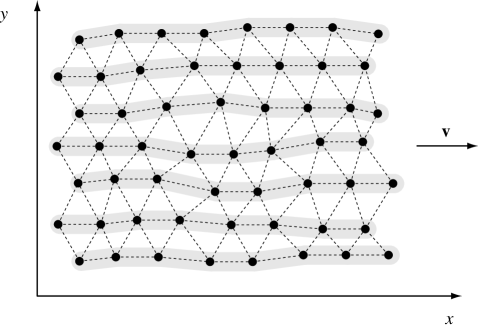
Figure 12: Structure of the moving vortex glass (intersection at constant ${\bf z}$). As long as the elastic glass is stable (in $d>2$ for sufficiently high drive and low temperature), the topological order of the lattice is preserved (dashed lines link neighbouring vortices). Although the moving vortex glass is rough (in $d\leq 3$ both displacement components have unbounded disorder-induced fluctuations) the vortices flow along channels (shaded lines, corresponding to the time-averaged vortex density).

Thus, in elastic approximation, the driven vortex lattice looks like a glass with respect to the structure, and hence one may call it ‘moving glass’ [Giamarchi and Le Doussal 1996]. Nevertheless, unlike the Bragg glass the ‘moving glass’ does not match all criteria of glassiness as specified in section 3.3. Since $u_{y}$ is quenched, one might expect to find a sub-linear transverse response, $\eta_{yy}({\bf v})=\left.{dF_{y}({\bf v})}/{dv_{y}}\right|_{v_{y}=0}=\infty$ at finite temperature. This is, however, not the case: a finite transverse force $F_{y}$ induces a linear transverse velocity $v_{y}$ [Le Doussal and Giamarchi 1998b, Scheidl and Vinokur 1998b]. Only at zero temperature there is a finite critical transverse force. But this is true for any potential and not indicative for the actual relevance of disorder for the dynamics.

The renormalization-group analysis reflects characteristic features of non-equilibrium, including the generation of Kardar-Parisi-Zhang (KPZ) nonlinearities, and an anisotropic renormalization of the elastic dispersion of the lattice, of the linear mobility and of the temperature [Balents et al. 1998a, Le Doussal and Giamarchi 1998b, Scheidl and Vinokur 1998b]. The detailed discussion of these aspects is beyond the scope of this article.

7.3 Moving smectic and dynamic melting

In the previous section we discussed the moving vortex system in the elastic approximation and found that is has long-range order in $d>3$, quasi-long-range order in $d=3$ and only short-range order in $d<3$. In order to examine whether this elastic system is actually stable with respect to the generation of free dislocations, it is in principle necessary to examine their dynamic generation process, since in the non-equilibrium situation the lattice stability can no longer be examined using energetic criteria.

Nevertheless, if we naively carry over our findings from equilibrium to non-equilibrium, we might expect the elastic system (the moving lattice, which is topologically ordered and where vortices move coherently) in $d\geq 3$ to be stable since it has (quasi-) long-range order, whereas the short-range order in $d<3$ should imply the instability. One can arrive at the same conclusion on the basis of a dynamical scaling analysis which was performed by [Balents and Fisher 1995] (?) for CDW systems.

[Balents et al. 1997] (?) argued that because of the dominance of fluctuations of $u_{x}$ over fluctuations of $u_{y}$ on largest scales, the instability should be generated by dislocations with Burgers vectors parallel to ${\bf v}$. Due to the presence of these dislocations the channels would be decoupled dynamically, i.e. vortices in different channels could move with locally different velocities. An analogous decoupling of charge-density waves in a layered model was found by [Vinokur and Nattermann 1997] (?) from a variational calculation.

Despite the dynamic decoupling it is possible that a static channel structure still persists. This phase is called ‘moving smectic’ [Balents et al. 1997] or ‘moving transverse glass’ [Le Doussal and Giamarchi 1998b]. The vortex density can still be modulated with quasi-long-range order in $d=3$. In $d<3$ it is possible that even this channel structure is destroyed, since the power-law roughness of $u_{y}$ may also induce dislocations with Burgers vectors having a component perpendicular to ${\bf v}$. Then the vortex system would be essentially a vortex liquid, which still has a certain anisotropy since the driving force breaks the rotation symmetry in the $(x,y)$ plane. Although the moving lattice can exist at sufficiently large drift velocities in $d=3$, the effective strength of disorder becomes larger as the velocity is reduced and therefore the moving lattice can decay first into a moving smectic and then into a moving liquid. The schematic phase diagrams [Balents et al. 1998a, Le Doussal and Giamarchi 1998b, Scheidl and Vinokur 1998b] for $d=2$ and $d=3$ are illustrated in figure 13.

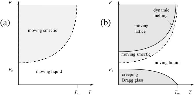
Figure 13: Schematic illustration of the dynamic phase diagram for vortex systems driven in disorder. (a) In $d=2$ dislocations are present in the vortex system for zero drive as well as for large drive. Thus at small drive the vortices form a liquid, for which is pinned only at $T=0$ and small drive $F<F_{\rm c}$. At large drive the moving vortices can start to follow static channels and to become a moving smectic. (b) In $d=3$ vortices form a Bragg glass below melting ($T<T_{\rm m}$) and below depinning ($F<F_{\rm c}$). For $F>0$ and $T>0$ this lattice will creep until the stresses in the lattice become very large such that the lattice breaks into a moving liquid. At $T=0$ this destruction of the solid presumably occurs very close to depinning. At larger drive, the moving liquid develops transverse order as in $d=2$. Unlike in $d=2$, the moving smectic can dynamically freeze into a moving lattice at even larger drive. In both dimensions the physics at intermediate drive ($F\simeq F_{\rm c}$) lacks a precise theoretical description because in this non-equilibrium regime disorder is effectively strong.

A theoretical analysis of the large-scale properties of the driven vortex system is hampered by the anisotropy of the system, the relevance of disorder and the dynamic non-linearities such as KPZ terms that govern the vortex dynamics on large scales. For these reasons a rigorous analysis has not been achieved so far. The conspiracy of these influences may actually lead to further phase transitions, such as first-order roughening transitions, which were found by [Chen et al. 1996] (?) for charge-density-wave systems in $d=1,2$.

There is experimental evidence not only for dynamic melting, but also the structure of the moving lattice and moving smectic have been characterized. The transition was detected by resistive measurements [Bhattacharya and Higgins 1993, Hellerqvist et al. 1996] and the structure of the dynamic phases was observed by dynamic decoration techniques [Marchevsky et al. 1997, Pardo et al. 1998, Troyanovskii et al. 1999]. Numerical evidence for dynamic melting was found in $d=2$ [Koshelev and Vinokur 1994, Ryu et al. 1996a, Faleski et al. 1996] and also $d=3$ [Domínguez et al. 1997].

In $d=2$ melting can show up only as a crossover which, however, may be very sharp for weak disorder and restricted system sizes. [Spencer and Jensen 1997] (?) presented numerical evidence for the absence of true topological order even at large velocity in $d=2$. The instability of the driven two-dimensional system was demonstrated analytically by [Aranson et al. 1998] (?) who explicitly examined the dynamics of single dislocations and their interaction within a driven vortex lattice. They were able to show that already the presence of the KPZ terms leads to a screening of the dislocation interaction on a finite length scale (which, however, increases exponentially with the drift velocity). Consequently, dislocation–anti-dislocation pairs will unbind under the additional influence of thermal fluctuations and even more due to the shaking effect of disorder.

In the remainder of this section we briefly readdress the melting transition and sketch how it can be captured by the conceptually simplest approach, a dynamical Lindemann criterion. Such a phenomenological approach can be useful in order to locate a transition semiquantitatively, but it certainly cannot give insight into large-scale properties. The Lindemann criterion will not be used for the total fluctuations of the vortex displacement, but for the relative displacement of neighbouring vortices. In this modified form it has proved to be successful in the static case even for systems which have no true long-range order, see equation (6.51). In order to extract information about the anisotropic nature of the driven state it is instructive to look at the relative displacement fluctuations

$$w^{2}({\bf b}) = \overline{\langle[{\bf u}({\bf b})-{\bf u}({\bf 0})]^{2}\rangle}$$ (7.23)

$$= w^{2}_{x}b_{x}^{2}/b^{2}+w^{2}_{y}b_{y}^{2}/b^{2}$$ (7.24)

as a function of the orientation of the vector ${\bf b}$ between the ideal position of the neighbours. [Scheidl and Vinokur 1998a] (?) evaluated the Lindemann criterion $w^{2}({\bf b})\leq c_{\rm Li}^{2}a^{2}$ for the stability of the lattice and determined the velocity dependence of the melting transition. In this context we will not reproduce the detailed results. But it is interesting to point out that pinning results in contributions

$$w_{x}^{2} \propto \frac{1}{v^{2}},$$ (7.25a)

$$w_{y}^{2} \propto \frac{1}{v}$$ (7.25b)

for the bond fluctuations, which imply that for large drift velocities nearest neighbours separated in $y$ direction have larger bond fluctuations than nearest neighbours in $x$ direction. Hence this phenomenological criterion indicates that the moving lattice (provided it exists at large drive) will decay into decoupled channels. This conclusion from the Lindemann criterion, which examines displacement fluctuations on short scales, is in agreement with the analysis of fluctuations on large scales described above. Concerning the resulting shift of the dynamic melting temperature it agrees with the finding (7.10) from the incoherent shaking temperature (7.8c). Thus the different approaches, the shaking temperature as measure of the strength of the pinning force, the Lindemann criterion as a measure of the displacement fluctuations on small scales and the renormalization-group results for the displacement fluctuations on large scales give in combination a consistent picture of the physics of driven vortices.

8 Summary

In this article we have reviewed the influence of weak pinning by point-like impurities on the vortex-line lattice in type-II superconductors. In particular, we have addressed the question to what extent these superconductors display glass-like properties and by which order parameter or correlation functions these properties can be identified.

Hereby it is important to distinguish two concepts of order: (i) order in the position of the vortex lines, which allows for a breaking of the continuous translational symmetry that is reflected by a spatial modulation of the magnetic induction; and (ii) the order of the superconducting condensate wave function, which is related to the breaking of the $U(1)$ symmetry and which manifests itself in phase coherence (ODLRO).

Pinning destroys the positional long-range order of the VLL in $d\leq 4$. However, for weak pinning (and for sufficiently low temperature, which is always assumed) quasi-long-range positional order persists in $2<d\leq 4$. This is true also in superconducting films ($d=2$) in a parallel field (where the exponent of the algebraic decay depends only logarithmically on the scale), but not in a perpendicular field, where dislocations induce short-ranged positional order.

In $d>2$ the vortex lattice behaves as an elastic medium for weak disorder, i.e., it is topologically ordered since there are no free dislocations. Then the vortex system can be called an elastic vortex glass. (A superconducting film in a parallel field can also be considered as an elastic glass since dislocations are excluded for geometrical reasons). In elastic vortex glasses vortices are collectively pinned such that vortex motion can take place only due to thermal activation over arbitrarily high barriers. Such barriers are necessary for a vanishing linear resistivity; otherwise the superconductor in the mixed phase would actually be an Ohmic conductor.

In the mixed phase vortex fluctuations are decisive not only for the degree of positional order in the vortex system but also for the phase coherence. In pure systems thermal fluctuation destroy ODLRO in $d\leq 4$ dimensions (if screening is taken into account), including bulk superconductors and superconducting films in a perpendicular field. Preliminary calculations to lowest order in $\epsilon$ for $d=4-\epsilon$ dimensions suggest that this conclusion remains true also for systems with weak disorder. A phase-coherent vortex glass, where the condensate wave function is quenched, can exist only in unphysical dimensions $d>4$. However, higher order terms in $\epsilon$ may still change this result. This applies in particular to systems with strong disorder (e.g. gauge-glass models without screening) that substantially suppresses thermal fluctuations and may permit the persistence of phase coherence in $d\leq 4$.

When the elastic vortex glass breaks down due to the proliferation of dislocations, it may still possess a weaker degree of order that might disappear only at higher temperatures and/or stronger disorder. Since the positional order of the elastic vortex glass in $2<d\leq 4$ resembles that of the pure crystal in $d=2$, it is possible that the elastic vortex glass breaks into a hexatic vortex liquid with bond-orientational order [Chudnovsky 1989, Toner 1991b] before it decays into an isotropic vortex liquid. A more detailed investigation of this possibility as well as of further more exotic disordered phases is left for future studies.

Appendix A Pinning of periodic media

In this appendix we present the transformation of the pinning energy for vortex line lattices, which leads to an effective periodic pinning potential. In our notation ${\bf r}=({\bf x},{\bf z})$ denotes a point of space, with the $D$-dimensional component ${\bf z}$ component along the vortex lines (in general dimension, a manifold) and the $N$-dimensional orthogonal component ${\bf x}$ of the displacement. The dimension of the embedding space of the VLL then is $d=N+D$. In the undistorted lattice, the vortex lines are located at positions ${\bf X}$. The distorted lattice can be described by the density (lines per $N$-dimensional volume)

$$\rho_{\bf u}({\bf r})=\sum_{{\bf X}^{\prime}}\delta({\bf x}-{{\bf X}^{\prime}}-{\bf u}({\bf X}^{\prime},{\bf z})).$$ (A.1)

The average density is denoted by $\rho_{0}$ and it is related to the average vortex spacing $a$ through $\rho_{0}=a^{-N}$. In particular, $\rho_{0}=B/\Phi_{0}$ for dimension $N=2$.

The pinning energy reads

$${\cal H}_{\rm pin} = \int d^{D}z\sum_{\bf X}V({\bf X}+{\bf u}({\bf X},{\bf z}),{\bf z})=\int d^{d}r\ \rho_{\bf u}({\bf r})V({\bf r})$$ (A.2)

We always assume disorder to be Gaussian distributed with correlations

$$\overline{V({\bf x},{\bf z})V({\bf x}^{\prime},{\bf z}^{\prime})}=\Delta({\bf x}-{\bf x}^{\prime})\delta({\bf z}-{\bf z}^{\prime}).$$ (A.3)

Using the Poisson-summation formula [Nattermann et al. 1991, Giamarchi and Le Doussal 1995], we may rewrite the density

$$\rho_{\bf u}({\bf r}) = \sum_{{\bf X}^{\prime}}\int d^{N}x^{\prime}\ \delta({\bf x}-{\bf x}^{\prime}-{\bf u}({\bf x}^{\prime},{\bf z}))\ \delta({\bf X}^{\prime}-{\bf x}^{\prime})$$ (A.4)

$$= \int d^{N}x^{\prime}\ \delta({\bf x}-{\bf x}^{\prime}-{\bf u}({\bf x}^{\prime},{\bf z}))\ \rho_{0}\sum_{\bf Q}e^{i{\bf Q}\cdot{\bf x}^{\prime}}$$

$$= {\rm det}^{-1}[\delta_{\alpha\beta}+\partial_{\alpha}u_{\beta}({\bf x},{\bf z})]\rho_{0}\sum_{\bf Q}e^{i{\bf Q}\cdot[{\bf x}-\widetilde{\bf u}({\bf r})]}$$

$$\approx [1-\partial_{\alpha}u_{\alpha}({\bf x},{\bf z})]\rho_{0}\sum_{\bf Q}e^{i{\bf Q}\cdot[{\bf x}-\widetilde{\bf u}({\bf r})]}$$

$$\approx -\rho_{0}\partial_{\alpha}u_{\alpha}({\bf x},{\bf z})+\rho_{0}\sum_{{\bf Q}}\cos\{{\bf Q}\cdot[{\bf x}-\widetilde{\bf u}({\bf r})]\},$$

where ${\bf Q}$ are reciprocal lattice vectors (RLV) and $\partial_{\alpha}=\partial/{\partial x_{\alpha}}$. The displacement tells us how vortices are shifted form the “ideal” position ${\bf x}^{\prime}$ to the “actual” position ${\bf x}$. In the beginning the displacement is considered as a function of the “ideal” position, ${\bf x}-{\bf x}^{\prime}={\bf u}({\bf x}^{\prime},{\bf z})$. During these manipulation we have expressed the displacement as a function of the actual position, ${\bf x}-{\bf x}^{\prime}=\widetilde{\bf u}({\bf x},{\bf z})$.

The random potential $V$ couples to the divergence of the displacement in the density, Eq. (A.4), as an effective random-compression force. This term is of particular importance in dimensions $d\leq 2$.

The remaining contributions ${\bf Q}\neq{\bf 0}$ to Eq. (A.4) represent an effective periodic pinning potential since it is invariant under shifts $\widetilde{\bf u}({\bf x},{\bf z})\to\widetilde{\bf u}({\bf x},{\bf z})+{\bf X}$ with an arbitrary lattice vector ${\bf X}$. However, since under this shift ${\bf x}$ is to be held fixed, the shift means ${\bf x}^{\prime}\to{\bf x}^{\prime}-{\bf X}$. Thus it does not mean a translation of the vortex lattice in the laboratory frame but it means as relabeling of the vortices, or a shift of the ideal reference positions ${\bf x}^{\prime}$.

In practice it is more convenient to start with the exact pinning energy for a VLL in the replicated system:

$${\cal H}_{{\rm pin},n} = -\frac{1}{2T}\sum_{a,b}\int d^{D}z\sum_{{\bf X},{\bf X}^{\prime}}\Delta({\bf X}+{\bf u}^{a}({\bf X},{\bf z})-{\bf X}^{\prime}-{\bf u}^{b}({\bf X}^{\prime},{\bf z}))$$ (A.5)

$$= -\frac{1}{2T}\sum_{a,b}\int d^{D}z\sum_{{\bf X},{\bf X}^{\prime}}\int_{\bf k}\widehat{\Delta}({\bf k})\ e^{i{\bf k}\cdot[{\bf X}+{\bf u}^{a}({\bf X},{\bf z})-{\bf X}^{\prime}-{\bf u}^{b}({\bf X}^{\prime},{\bf z})]},$$

where $\int_{\bf k}=\int d^{d}k/(2\pi)^{d}$ and the Fourier transform of the correlator is

$$\widehat{\Delta}({\bf k})\equiv\int d^{N}x\ e^{-i{\bf k}\cdot{\bf x}}\Delta({\bf x}).$$ (A.6)

The energy (A.5) can then be transformed in the following way: the wave vector ${\bf k}={\bf Q}+{\bf q}$ is split into a reciprocal lattice vector ${\bf Q}$ and a vector ${\bf q}$ within the first Brillouin zone and $\int_{\bf k}=\sum_{\bf Q}\int_{\bf q}$, accordingly. The contribution ${\bf Q}={\bf 0}$ represents the pinning energy for a continuous elastic medium. This contribution contains a random compression force (the terms of order $q^{2}$ in this contribution) which we will not discuss further here. We focus on the contributions ${\bf Q}\neq{\bf 0}$ which encode the periodicity of the VLL. For a short disorder correlation length $\xi\ll a$ one may approximate $\widehat{\Delta}({\bf Q}+{\bf q})\approx\widehat{\Delta}({\bf Q})$ and then perform the the integration over ${\bf q}$, after which only the contributions ${\bf X}={\bf X}^{\prime}$ survive since $|{\bf u}^{a}({\bf X},{\bf z})-{\bf u}^{b}({\bf X}^{\prime},{\bf z})|\ll|{\bf X}-{\bf X}^{\prime}|$ for a roughness exponent $\zeta<1$. After these approximations one ends up with

$${\cal H}_{{\rm pin},n} \approx -\frac{1}{2T}\sum_{a,b}\int d^{D}z\sum_{{\bf X}}\rho_{0}\sum_{\bf Q}\Delta({\bf Q})e^{i{\bf Q}\cdot[{\bf u}^{a}({\bf X},{\bf z})-{\bf u}^{b}({\bf X},{\bf z})]}$$ (A.7)

$$= -\frac{1}{2T}\sum_{a,b}\int d^{D}z\sum_{{\bf X}}a^{N}\widetilde{\Delta}({\bf u}^{a}({\bf X},{\bf z})-{\bf u}^{b}({\bf X},{\bf z}))$$

$$\approx -\frac{1}{2T}\sum_{a,b}\int d^{d}r\ \widetilde{\Delta}({\bf u}^{a}({\bf r})-{\bf u}^{b}({\bf r}))$$

with the effective periodic correlator

$$\widetilde{\Delta}({\bf u}) = \rho_{0}^{2}\sum_{\bf Q}\Delta({\bf Q})e^{i{\bf Q}\cdot{\bf u}}=\rho_{0}\sum_{\bf X}\Delta({\bf X}+{\bf u}),$$ (A.8)

which is related to the effective potential via

$$\overline{\widetilde{V}({\bf u},{\bf r})\widetilde{V}({\bf u}^{\prime},{\bf r}^{\prime})}\approx\widetilde{\Delta}({\bf u}-{\bf u}^{\prime})\delta({\bf r}-{\bf r}^{\prime}).$$ (A.9)

This means that the periodic lattice effectively behaves like an elastic manifold of internal dimension $D_{\rm eff}=D+N$ in a effective embedding space $d_{\rm eff}=D+2N$ subject to a periodic pinning potential.

The advantage of the manipulations (A.7) as compared to (A.4) is that we end up with a periodic correlator for the displacement ${\bf u}$ as a function of the ideal reference position (which is the actual degree of freedom of the vortex lattice) rather than for $\widetilde{\bf u}$ as a function of the actual vortex position.

Appendix B List of recurrent symbols

symbol	meaning	definition
$a$	effective vortex spacing	$a^{2}\equiv\Phi_{0}/B$
$a_{\triangle}$	vortex spacing in triangular lattice	$a_{\triangle}^{2}\equiv(2/\sqrt{3})a^{2}$
${\bf A}$	magnetic vector potential
${\bf B}$	magnetic induction
$c$	velocity of light
$c_{\rm g}$, $c_{1}$, $c_{2}$, …	numerical constants
$c_{11}$	compression modulus
$c_{44}$	tilt modulus
$c_{66}$	shear modulus
$c_{\rm Li}$	Lindemann number	(2.21)
$C_{\rm VG}$	phase-coherent vortex-glass correlation	(2.34)
$d$	(total) spatial dimension	page 3
$D$	(internal) spatial dimension	page 3
${\cal E}$	energy
${\bf F}$	driving force	(3.51)
${\cal F}$	free energy
$G$	displacement response function	(3.11)
${\rm Gi}$	Ginzburg number	(2.5)
${\bf H}$	magnetic field
$H_{\rm c}$	thermodynamic critical field	page 2.1
$H_{\rm c1}$	lower critical field	page 2.2
$H_{\rm c2}$	upper critical field	page 2.1
$H_{\rm m1}$	lower melting field	page 2.22
$H_{\rm m2}$	upper melting field	(2.23)
${\cal H}$	Hamiltonian
$j$	current density
$J$	effective stiffness	(4.16b)
${\bf k}$	wave vector, without restriction	${\bf k}={\bf Q}+{\bf q}$
$L$	system size
$L_{a}$	crossover length	(6.2)
$L_{\rm s}$	screening length	(5.3)
$L_{\xi}$	Larkin length	(3.16), (LABEL:def.L.R_xi)
$n$	number of replicas
$N$	number of displacement components	page 3
${\bf P}^{L/T}$	longitudinal/transverse projector	(5.1)
${\bf q}$	wave vector, restricted to first Brillouin zone
${\bf Q}$	reciprocal lattice vector (RLV)
${\cal Q}$	thermodynamic quantity	(2.17)
$Q_{\triangle}$	length of first RLV in triangular lattice	$Q_{\triangle}^{2}\equiv 16\pi^{2}/3a_{\triangle}^{2}$
$R_{a}$	crossover length	(6.2)
$R_{t}$	rescaled length	(6.40)
$R_{\xi}$	Larkin length	(LABEL:def.L.R_xi)
$s$	film thickness
$S$	translational order parameter correlation	(2.33), (3.9)
$S_{\rm PG}$	positional glass correlation	(2.33)
$\widehat{S}$	structure factor	(4.35)
${\cal S}$	entropy
$T_{\rm c}$	superconducting transition temperature
$T_{\rm c0}$	mean-field transition temperature	page 2.1
$T_{\rm g}$	glass transition temperature	(4.25), (5.23)
$T_{\rm h}$	hexatic/isotropic liquid transition temperature	(5.14)
$T_{\rm m}$	melting temperature	(5.10)
$T_{\rm KT}$	Kosterlitz-Thouless transition temperature	(5.4)
${\bf u}$	vortex displacement
$U$	interaction potential
${\bf v}$	velocity
$V$	pinning potential
$W$	variance of displacement difference	(3.6), (3.10)
$x$	component of ${\bf x}$ parallel to ${\bf v}$
${\bf x}$	vector component perpendicular to ${\bf B}$
$y$	component of ${\bf x}$ perpendicular to ${\bf v}$
${\bf z}$	vector component parallel to ${\bf B}$
$z$	dynamical exponent	(4.52)
$z_{l}$, $z_{t}$	rescaled lengths	(6.10)
$\gamma$	ratio of elastic constants	$\gamma\equiv c_{66}/c_{11}$, (6.5)
${\gamma_{\rm Eu}}$	Euler’s constant	${\gamma_{\rm Eu}}=0.577\cdots$
$\Gamma$	elastic dispersion relation	(LABEL:intro.dispers)
$\delta$	anisotropy parameter	(6.26)
$\Delta$	disorder correlator	(3.3)
$\Delta_{0}$	integral of disorder correlator	(3.4)
$\Delta^{(2)}$	moment of disorder correlator	(3.13)
$\widetilde{\Delta}$	periodic disorder correlator	(A.8)
$\widetilde{\Delta}^{(2)}$	moment of periodic disorder correlator	page 6.21, (6.25)
$\epsilon$	anisotropy	page 2.2
$\epsilon$	dimension	$\epsilon=4-D$
$\varepsilon_{0}$	energy scale	(5.2)
$\varepsilon_{\parallel}$	stiffness of manifold	(3.1)
$\zeta$	roughness exponent	(3.6)
${{\zeta}}$	thermal noise	(3.51)
$\zeta_{\rm F}$	Flory roughness exponent	(3.20)
$\zeta_{\rm rf}$	random force roughness exponent	(3.15)
$\zeta_{\rm rfi}$	random field roughness exponent	(3.27)
$\zeta_{\rm rm}$	random manifold roughness exponent	(3.23)
$\zeta_{\rm th}$	thermal roughness exponent	(3.7)
$\eta$	correlation exponent	(4.33)
$\eta_{0}$	unrenormalized friction coefficient	(3.51)
$\theta$	scaling exponent of energy fluctuations	(3.18)
$\kappa$	Ginzburg-Landau parameter	$\kappa\equiv\lambda/\xi$
$\lambda$	magnetic penetration length	(2.2b)
$\Lambda_{T}$	thermal length	(2.19)
$\mu$	random tilt	(3.24)
$\mu$	creep exponent	(3.70b)
$\mu_{\rm mag}$	magnetic permeability	(4.43)
$\xi$	coherence length	(2.2a)
$\xi$	disorder correlation length
$\Xi$	pinning force correlator	(LABEL:intro.Xi)
$\rho$	vortex density	(4.10)
$\rho_{0}$	average vortex density	$\rho_{0}=B/\Phi_{0}$
$\rho_{\rm n}$	normal state resistivity	(3.50)
$\sigma$	random tilt strength	(4.18b)
$\tau$	relative temperature distance	$\tau\equiv 1-T/T_{\rm g}$, (4.27)
$\Phi_{0}$	flux quantum	$\Phi_{0}\equiv hc/2e$
$\psi$	barrier scaling exponent	(3.46)
$\psi_{\bf k}$	translational order parameter	(3.8)

Note that functions and their Fourier transforms have the same name although they are different functions. This ambiguity is removed by the argument of the function, which is either a length (such as ${\bf x}$, ${\bf z}$, ${\bf r}$ etc.) or a wave vector (such as ${\bf k}$, ${\bf q}$, ${\bf Q}$ etc.). The only exceptions are $\Delta$ and $\widetilde{\Delta}$. Their common Fourier transform is denoted by $\widehat{\Delta}$.

References

- Abrikosov 1957 Abrikosov, A. A., 1957, Sov. Phys. JETP, 5, 1174.
- Abrikosov 1964 Abrikosov, A. A., 1964, Sov. Phys. JETP, 19, 988.
- Affleck and Brézin 1985 Affleck, I. and Brézin, E., 1985, Nucl. Phys. B, 257, 451.
- Aharony and Harris 1996 Aharony, A. and Harris, A. B., 1996, Phys. Rev. Lett., 77, 3700.
- Alonso and Fernandez 1999 Alonso, J. J. and Fernandez, J. F., 1999, Phys. Rev. E, 59, 2659.
- Anderson and Kim 1964 Anderson, P. W. and Kim, Y. B., 1964, Rev. Mod. Phys., 36, 39.
- Aranson et al. 1998 Aranson, I. S., Scheidl, S. and Vinokur, V. M., 1998, Phys. Rev. B, 58, 14541.
- Bagchi et al. 1966 Bagchi, K., Anderson, H. C. and Swope, W., 1966, Phys. Rev. Lett., 76, 255.
- Balents and Fisher 1993 Balents, L. and Fisher, D. S., 1993, Phys. Rev. B, 48, 5949.
- Balents and Fisher 1995 Balents, L. and Fisher, M. P. A., 1995, Phys. Rev. Lett., 75, 4270.
- Balents and Kardar 1993 Balents, L. and Kardar, M., 1993, Nucl. Phys. B, 393, 480.
- Balents et al. 1997 Balents, L., Marchetti, M. C. and Radzihovsky, L., 1997, Phys. Rev. Lett., 78, 751.
- Balents et al. 1998a Balents, L., Marchetti, M. C. and Radzihovsky, L., 1998a, Phys. Rev. B, 57, 7705.
- Balents et al. 1998b Balents, L., Radzihovsky, L. and Fisher, D. S., 1998b, Private communication.
- Bardeen and Stephen 1965 Bardeen, J. and Stephen, M. J., 1965, Phys. Rev., 140, 1197A.
- Batrouni and Hwa 1994 Batrouni, G. G. and Hwa, T., 1994, Phys. Rev. Lett., 72, 4133.
- Bauer and Bernard 1996 Bauer, M. and Bernard, D., 1996, Europhys. Lett., 33, 255.
- Baym 1995 Baym, G., 1995, Phys. Rev. B, 51, 11697.
- Bednorz and Müller 1986 Bednorz, J. G. and Müller, K. A., 1986, Z. Phys. B, 64, 189.
- Belanger and Young 1991 Belanger, D. P. and Young, A. P., 1991, J. Magn. Magn. Mat., 100, 272.
- Berghuis et al. 1990 Berghuis, P., van der Slot, A. L. F. and Kes, P. H., 1990, Phys. Rev. Lett., 65, 2583.
- Bhattacharya and Higgins 1993 Bhattacharya, S. and Higgins, M. J., 1993, Phys. Rev. Lett., 70, 2617.
- Binder and Young 1986 Binder, K. and Young, A. P., 1986, Rev. Mod. Phys., 58, 801.
- Blatter et al. 1994 Blatter, G., Feigel’man, M. V., Geshkenbein, V. B., Larkin, A. I. and Vinokur, V. M., 1994, Rev. Mod. Phys., 66, 1125.
- Blatter and Geshkenbein 1996 Blatter, G. and Geshkenbein, V., 1996, Phys. Rev. Lett., 77, 4958.
- Blatter et al. 1992 Blatter, G., Geshkenbein, V. B. and Larkin, A. I., 1992, Phys. Rev. Lett., 68, 875.
- Bogner et al. 2000 Bogner, S., Emig, T. and Nattermann, T., 2000, Unpublished.
- Bokil and Young 1995 Bokil, H. S. and Young, A. P., 1995, Phys. Rev. Lett., 74, 3021.
- Bolle et al. 1999 Bolle, C. A., Aksyuk, V., Pardo, F., Gammel, P. L., Zeldov, E., Buchner, E., Boie, R., Bishop, D. J. and Nelson, D. R., 1999, Nature (London), 399, 43.
- Bonsall and Maradudin 1977 Bonsall, L. and Maradudin, A. A., 1977, Phys. Rev. B, 15, 1959.
- Bouchaud et al. 1995 Bouchaud, J.-P., Mézard, M. and Parisi, G., 1995, Phys. Rev. E, 52, 3656.
- Bouchaud et al. 1991 Bouchaud, J.-P., Mézard, M. and Yedidia, J. S., 1991, Phys. Rev. Lett., 67, 3840.
- Bouchaud et al. 1992 Bouchaud, J.-P., Mézard, M. and Yedidia, J. S., 1992, Phys. Rev. B, 46, 14686.
- Boyanovsky and Cardy 1982 Boyanovsky, D. and Cardy, J., 1982, Phys. Rev. B, 25, 7058.
- Brandt 1974 Brandt, E. H., 1974, Phys. Status Solidi, 64, 257.
- Brandt 1977a Brandt, E. H., 1977a, J. Low Temp. Phys., 26, 709.
- Brandt 1977b Brandt, E. H., 1977b, J. Low Temp. Phys., 28, 263.
- Brandt 1989 Brandt, E. H., 1989, Phys. Rev. Lett., 63, 1106.
- Brandt 1991 Brandt, E. H., 1991, Int. J. Mod. Phys. B, 5, 751.
- Brandt 1995 Brandt, E. H., 1995, Rep. Prog. Phys., 58, 1465.
- Brandt et al. 1996 Brandt, E. H., Mints, R. G. and Snapiro, I. B., 1996, Phys. Rev. Lett., 76, 827.
- Bray 1974 Bray, A. J., 1974, Phys. Rev. B, 9, 4752.
- Brézin et al. 1990a Brézin, E., Fujita, A. and Hikami, S., 1990a, Phys. Rev. Lett., 65, 1949 [Erratum: [Brézin et al. 1990b]].
- Brézin et al. 1990b Brézin, E., Fujita, A. and Hikami, S., 1990b, Phys. Rev. Lett., 65, 2921.
- Brézin et al. 1985 Brézin, E., Nelson, D. R. and Thiaville, A., 1985, Phys. Rev. B, 31, 7124.
- Bruinsma and Aeppli 1984 Bruinsma, R. and Aeppli, G., 1984, Phys. Rev. Lett., 52, 1547.
- Calliol et al. 1982 Calliol, J. M., Levesque, D., Weis, J. J. and Hansen, J. P., 1982, J. Stat. Phys., 28, 325.
- Cardy and Ostlund 1982 Cardy, J. L. and Ostlund, S., 1982, Phys. Rev. B, 25, 6899.
- Carpentier 1999 Carpentier, D., 1999, Défauts topologiques en présence de désordre Ph.D. thesis, ENS Paris.